Abstract

We present a dynamical model of lipoprotein metabolism derived by combining a cascading process in the blood stream and cellular level regulatory dynamics. We analyse the existence and stability of equilibria and show that this low-dimensional, nonlinear model exhibits bistability between a low and a high cholesterol state. A sensitivity analysis indicates that the intracellular concentration of cholesterol is robust to parametric variations while the plasma cholesterol can vary widely. We show how the dynamical response to time-dependent inputs can be used to diagnose the state of the system. We also establish the connection between parameters in the system and medical and genetic conditions.

A Dynamical Model of Lipoprotein Metabolism

E. August, K.H. Parker and M. Barahona

1 Introduction

We model the dynamics of lipoprotein metabolism associated with the transport of lipids in the blood. The malfunction of the delivery of lipids and cholesterol from the liver to the cells has important ramifications. There is strong medical evidence linking high plasma concentrations of low-density lipoproteins (LDL) to the development of atherosclerosis, the deadliest disease in industrialised countries (Glass and Witztum, 2001; Rodríguez et al., 1999; Libby, May 2002). However, LDL is just one species in a metabolic cascade by which different lipoproteins (Table 1) are synthesised, degraded and absorbed. In this complex network, it is important to investigate how metabolic control is exercised and if dynamical features, other than high LDL concentrations, could be useful markers for the detection of disease states.

Previous modelling efforts of lipoprotein metabolism vary in scope. Some models have concentrated on detailed aspects of the system, such as the fluid dynamics of lipid accumulation on the arterial walls (Hazel and Pedley, 1998) or the chemical kinetics of LDL oxidation (Cobbold et al., 2002), but do not describe the processes at the cellular or physiological level. Other approaches have modelled the lipoprotein network as a whole with linear compartmental models (Jacquez, 1985; Pont et al., 1998; Parhofer et al., 1991). Although these models can be fitted to match experimental data, the compartments lack rigorous physiological meaning, thus making it difficult to describe the underlying biochemical processes. For instance, compartments added to represent subclasses of lipoproteins can always be reduced to one compartment because of the linearity of the models (Eisenfled and Grundy, 1984).

Our model of lipoprotein metabolism is a relatively low-dimensional system of nonlinear differential equations which are strongly linked to the underlying physiological processes. The system can undergo a transition between low and high LDL steady states, a feature which is robust to randomness and uncertainty in the parameters. Because the equations are directly related to physiological processes, the model can be used to study the effect of genetic or behavioral conditions and could serve as an aid to test hypotheses for diagnosis and intervention. In what follows, we derive our model from the main physiological processes; we then analyse the system and carry out a sensitivity analysis; finally, we show how the results can be related to experiments and medical conditions.

2 Modelling Lipoprotein Metabolism

Lipoproteins constitute the primary means of transport of lipids from the liver to the cells via the blood stream. Lipoprotein dynamics is intimately connected to lipid and cholesterol metabolic networks. Figure 1 provides a schematic overview of the origin, transport and fate of the different lipoproteins in the human body at two levels: the macroscopic and the cellular.

Lipoproteins are globular aggregates of lipids and proteins: cholesterol ester and triacylglycerol form the core; amphiphilic phospholipids surround them forming the hull; and different apolipoproteins (apo A, apo B, apo C, and apo E), which function as trigger-molecules for specific reactions, are embedded in the surface. Lipoproteins are classified in five standard groups (Table 1), based on density and the apolipoproteins attached to them. In increasing order of density and decreasing order of size (the fewer lipids relative to its size, the denser the lipoprotein is): chylomicrons (Chyl), very low-density lipoproteins (VLDL), intermediate-density lipoproteins (IDL), low-density lipoproteins (LDL), and high-density lipoprotein (HDL).

	Chyl	VLDL	IDL	LDL	HDL
Density ($g/ml$)	$<$ 0.95	0.95–1.006	1.006–1.019	1.019–1.063	1.063–1.21
Diameter ($nm$)	80–100	30–80	25–30	20–25	8–13
Cholesterol (%)	3–5	12–21	27–46	40–50	15–25
Apolipoproteins	A, C, E, B-48	C, E, B-100	C, E, B-100	B-100	A, C, E

Table 1: The properties and composition of the five standard lipoprotein classes (Adiels, 2002): chylomicrons (Chyl), very low-density lipoproteins (VLDL), intermediate-density lipoproteins (IDL), low-density lipoproteins (LDL), and high-density lipoproteins (HDL).

Chylomicrons contain a large proportion of fatty acids and are found in the blood stream mainly after digestion of a meal. They are synthesised by the intestines and constitute the direct means by which dietary fat is delivered to heart, muscle, and adipose tissue. Chylomicrons provide the liver with lipids and proteins but are not regulated by the liver. Therefore, we do not consider the concentration of chylomicrons as an explicit variable in our model and include their effect parametrically as an input of lipids to the system.

The liver is responsible for the secretion of all other lipoproteins, most significantly VLDL. (Although small amounts of IDL and LDL are produced by the liver, we neglect this contribution.) VLDL is secreted by the liver into the blood at an almost constant rate (slightly higher during the night) as a means of transport of synthesised fat and cholesterol to peripheral tissues. While in the blood stream, the apo C protein on the surface of VLDL can bind to the extracellular enzyme lipoprotein lipase (LPL), which is present on the capillary wall. The effect of LPL is to hydrolyse triacylglycerol, thus reducing the size of VLDL and increasing the percentage of denser molecules (i.e., it degrades VLDL to IDL). After hydrolysis, the fatty acids are taken up by nearby cells or by serum albumin for transport to more peripheral cells. A similar process leads from IDL to LDL. This is the lipoprotein cascade that transforms VLDL into IDL into LDL. (This process also involves losing apo C and apo A to HDL, which is independently synthesised in the liver and is not a part of the lipoprotein cascade.)

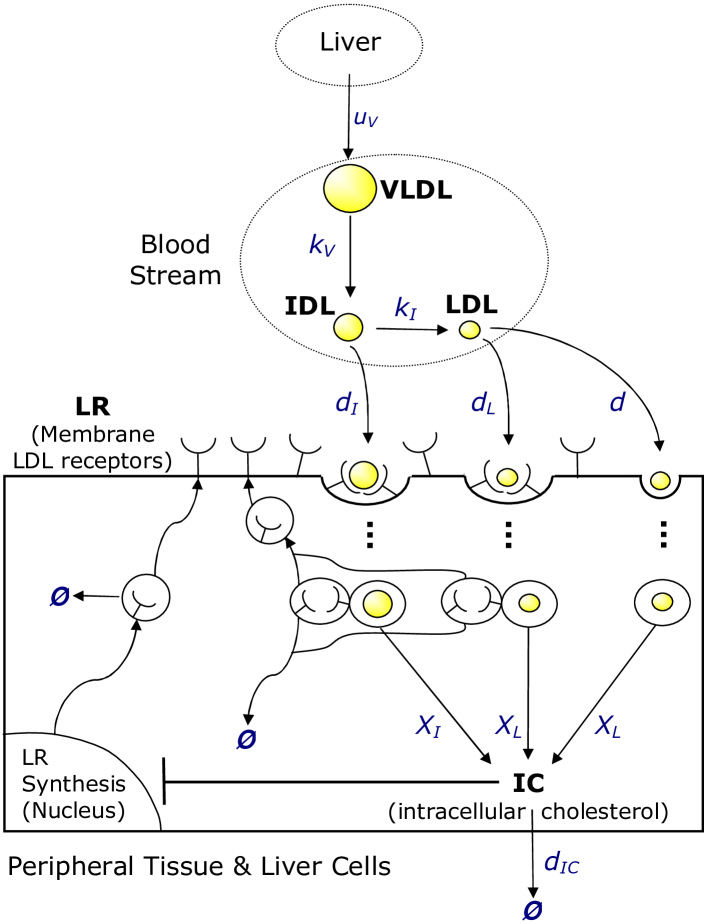
Figure 1: Overview of origin, transport and fate of lipoproteins. A schematic view of the processes involved in the metabolism of lipoproteins at both the macroscopic and cellular levels. The liver secretes VLDL at a rate $u_{V}$. The turnover rates of VLDL and IDL in the blood stream are $k_{V}$ and $k_{I}$, respectively. At the cellular level, $d_{L}$ and $d_{I}$ denote rate constants of the receptor-mediated uptake of lipoproteins: IDL and LDL bind to membrane receptors (LR), which cluster in coated pits in the cell membrane. Note that it is also possible for LDL (but not for IDL) to be absorbed directly through a non-receptor mediated path with rate constant $d$. After endocytic vesicles are formed and internalised, the lipoproteins are hydrolysed in the cell releasing lipids into the cytoplasm. A significant proportion of these lipids ($\chi_{I}$ in IDL and $\chi_{L}$ in LDL) is cholesterol which contributes to the level of intracellular cholesterol (IC). The intracellular cholesterol is used for cell function or eliminated, mainly through the action of HDL, at a rate $d_{IC}$. Most of the LDL receptors (but not all) are reincorporated into the membrane. In addition, the nuclear synthesis of the receptors LR is regulated through negative feedback ($\vdash$) by the intracellular cholesterol IC.

About 50% of the IDL and 75% of LDL in the blood are absorbed by hepatic and peripheral cells via LDL receptors (LR) on the cell membrane. These receptors are synthesised by the cell and recognise apo B and apo E with high affinity. In liver cells, the absorbed LDL is reused for lipoprotein synthesis and excess cholesterol is secreted into bile. In non-hepatic cells, the absorbed LDL supplies the cholesterol content essential for cell function (White and Baxter, 1984; Chopra and Thurnham, 1999). Although almost every cell can synthesise cholesterol to some extent, we assume that all cholesterol has to be delivered to the cells via LDL or IDL absorption (Mathews et al., 2000; Cooper, 2000; Converse and Skinner, 1992; Dietschy et al., 1978).

As mentioned above, there is another important component in the lipoprotein network: HDL (the “good cholesterol”), which is also secreted by the liver. HDL is responsible for reverse cholesterol transport, the transport of excess cholesterol from cells and other lipoproteins back to the liver. The effect of HDL is included in our model through a rate constant that parameterises the elimination of intracellular cholesterol, which is significantly affected by the HDL pathway.

The above processes can be modelled with the following system of differential equations, where $[\cdot]$ denotes concentration and $\phi_{LR}$ is the dimensionless fraction of total possible LDL receptors:

$$\frac{d[VLDL]}{dt} =-k_{V}[VLDL]+u_{V}$$ (1)

$$\frac{d[IDL]}{dt} =k_{V}[VLDL]-k_{I}[IDL]-d_{I}[IDL]\phi_{LR}$$ (2)

$$\frac{d[LDL]}{dt} =k_{I}[IDL]-d_{L}[LDL]\phi_{LR}-d[LDL]$$ (3)

$$\frac{d\phi_{LR}}{dt} =-b\left(d_{I}[IDL]+d_{L}[LDL]\right)\phi_{LR}+c\frac{1-\phi_{LR}}{[IC]}$$ (4)

$$\frac{d[IC]}{dt} =\left(\chi_{I}d_{I}[IDL]+\chi_{L}d_{L}[LDL]\right)\phi_{LR}+\chi_{L}d[LDL]-d_{IC}[IC].$$ (5)

The linear terms $k_{V}[VLDL]$ and $k_{I}[IDL]$ in (1)–(3) correspond to the cascade degradation of VLDL to IDL to LDL assuming saturated kinetics (i.e., excess of LPL enzyme) for the reactions. An implicit assumption is that the blood flow does not play a significant role in the absorption process. This is based on our analysis of the relevant time scales and also on detailed calculations of mass transfer in tissue under physiological conditions (Zhang, 2005).

Equation (1) contains the only input to the system, $u_{V}$, which represents the overall secretion rate of VLDL by the liver. High values of $u_{V}$ are associated with a high dietary intake of fats (Spady et al., 1993). On the other hand, medication with statins would reduce $u_{V}$ by lowering the synthesis of cholesterol and VLDL in the liver.

The nonlinear terms $d_{I}[IDL]\phi_{LR}$ and $d_{L}[LDL]\phi_{LR}$ represent the endocytosis of IDL and LDL via a process involving LDL receptors (LR) and leading to the release of lipids and cholesterol into the cytoplasm. This can be modelled in its simplest, classical form through a second order reaction  (Bywater et al., 2002). In addition to this receptor-mediated uptake, mammalian cells can take up LDL (but not IDL) by non-specific endocytosis at a rate $d[LDL]$, linearly proportional to its plasma (or extracellular) concentration (Hobbs et al., 1990; Willnow et al., 1999; Glass and Witztum, 2001; Goldstein and Brown, 1997). Endocytosis is greatly reduced under the genetic disease familial hypercholesterolemia (Section 4.1.3).

The last two equations (4)–(5) describe cholesterol uptake and regulation at the cellular level. The variables are: $\phi_{LR}$, the fraction of the total possible LDL receptors that mediate IDL and LDL endocytoses; and $[IC]$, the concentration of cellular cholesterol, which closes the loop by acting as a cellular control for the expression and synthesis of the LDL receptors, LR.

Parameter	Source	Units	Nominal Value	Range
$k_{V}$	(Packard et al., 2000)	$h^{-1}$	$0.3$	0.15–0.6
$k_{I}$	(Packard et al., 2000)	$h^{-1}$	$0.1$	0.025–0.1
$d_{I}$	—	$h^{-1}$	$1.4$	0.5–2
$d_{L}$	—	$h^{-1}$	$0.005$	0.005–0.02
$d$	(Dietschy et al., 1993)	$h^{-1}$	0.0025	0.0025-0.0075
$b$	—	$lg^{-1}$	$0.1$	0–2
$c$	(Goldstein and Brown, 1977)	$g(lh)^{-1}$	$0.05$	0–1
$\chi_{I}$	(Adiels, 2002)	–	0.35	0.25–0.45
$\chi_{L}$	(Adiels, 2002)	–	0.45	0.4–0.5
$u_{V}$	(White and Baxter, 1984)	$g(lh)^{-1}$	$0.3$	Variable
$d_{IC}$	(White and Baxter, 1984)	$h^{-1}$	$0.45$	Variable

Table 2: Parameters of the model (1)-(5). Nominal values and ranges as found in the literature. The nominal values for $d_{I}$ and $d_{L}$ are obtained by assuming that all other parameters are at nominal values and the equilibrium point of the linearised system in the lower branch of Eq. (17) is that of normal individuals (White and Baxter, 1984): $[VLDL]=1\,gl^{-1}$, $[IDL]=0.2\,gl^{-1}$, $[LDL]=2\,gl^{-1}$. The nominal values for $u_{V}$ and $d_{IC}$ are crude estimates from the cited reference. Because of their high dependence on diet, medication and genetic factors, we consider $u_{V}$ and $d_{IC}$ as the control parameters.

Eq. (4) reflects the dynamical processes involving the LDL surface receptors, which take part in the endocytotic reactions. Experiments in normal individuals indicate that the maximum number of receptors on the surface of the cell is $15,000-70,000$ per cell (Goldstein and Brown, 1977). The variable $\phi_{LR}$ represents the fraction of the total possible surface receptors that are present on the surface of the cell. Therefore, $\phi_{LR}$ is a surface occupancy fraction; hence it is dimensionless and bounded ($0\leq\phi_{LR}\leq 1$). Biological evidence indicates that most (but not all) of the receptors used in the endocytosis are reintegrated into the cell membrane. The first term in (4), weighted by a factor $b$, represents the loss of LDL receptors that are not recycled. The last term in (4) describes the cholesterol-regulated synthesis of LDL receptors and the process of their attachment to the surface of the cell. Further biological evidence indicates that cells regulate the synthesis of LDL receptors to prevent the over-accumulation of intracellular cholesterol. When grown in the presence of different concentrations of LDL, cells adjust the number of LDL receptors to take up only enough LDL to satisfy the cholesterol requirement for membrane turnover (Goldstein and Brown, 1977); when grown in total absence of LDL, the maximum number of possible surface LDL receptors is reached after 2–3 days. We have modelled this inhibitory mechanism with a simple reciprocal feedback: the synthesis of cytosolic LDL receptors is inversely proportional to the intracellular cholesterol $[IC]$. Furthermore, the attachment of the cytosolic LDL receptors to the cell surface can be described in its simplest form with a rate that is proportional to the fraction of unoccupied receptor sites $(1-\phi_{LR})$. The combined rate at which $\phi_{LR}$ increases is then given by the product $c(1-\phi_{LR})/[IC]$, where $c$ modulates the weight of the combined process of regulated synthesis and attachment. However, we emphasise that the qualitative results of the model do not depend on the particular form of the feedback chosen, as we discuss at the end of Section 3.2. For a more detailed explanation of this term see Appendix A.

Finally, Eq. (5) establishes the balance of flows of the cellular cholesterol $[IC]$. The parameters $0<\chi_{I}<\chi_{L}<1$ are the proportions of cholesterol in IDL and LDL, respectively, which can be measured experimentally. The last term in the equation $d_{IC}[IC]$ represents the outflow rate of cholesterol from the cell. This is largely related to the HDL-mediated reverse cholesterol transport, but also accounts for the cholesterol used by cells for their metabolism or eliminated through bile secretion in the liver. Therefore, our model parameterises the effect of HDL through the constant $d_{IC}$. As in the case of $u_{V}$, $d_{IC}$ will be a highly variable control parameter which can be affected by diet and statins.

The model has eleven parameters with nominal values and ranges shown in Table 2:

Model parameters: $k_{V},\ k_{I},\ d_{I},\ d_{L},\ d,\ b,\ c,\ \chi_{I}$, and $\chi_{L}$. These will differ between individuals but are assumed to remain virtually unchanged for an individual except for slow changes (e.g., with age). We have found values and estimates in the literature for all of these parameters, except for $b$ for which we assume $b=0.1$. Sensitivity analyses will be performed to check that the qualitative results are robust to variations in these parameters.

Control parameters: $u_{V}$ and $d_{IC}$. The secretion rate of VLDL from the liver ($u_{V}$) and the depletion rate of intracellular cholesterol ($d_{IC}$) are highly variable parameters and affected by genetic factors, diet and medication. Hence, we will consider these as the control parameters for our analysis.

3 Model Analysis: Fixed Points and Sensitivity Analysis

3.1 The System at Equilibrium

We have carried out a numerical analysis of the bifurcations and fixed points of the dynamical system (1)–(5). Before presenting the numerics, we briefly note some analytical features of the model.

The system is effectively four-dimensional since $[VLDL]$ converges exponentially to its equilibrium value $[VLDL]_{eq}=u_{V}/k_{V}$. Moreover, we can restrict our analysis to the non-negative orthant because the system is essentially non-negative, i.e., solutions remain non-negative for non-negative initial conditions (Haddad et al., 2001). The equilibrium point can also be bounded from above using the nullclines of (1)–(5) to give:

$$\frac{u_{V}}{k_{I}+d_{I}}\leq [IDL]_{eq} \leq\frac{u_{V}}{k_{I}}$$ (6)

$$\frac{k_{I}\,u_{V}}{(k_{I}+d_{I})(d+d_{L})}\leq [LDL]_{eq} \leq\frac{u_{V}}{d}$$ (7)

$$0\leq \phi_{LR_{eq}} \leq 1$$ (8)

$$\frac{\chi_{I}d_{I}+\chi_{L}k_{I}}{k_{I}+d_{I}}\frac{u_{V}}{d_{IC}}\leq [IC]_{eq} \leq\frac{\chi_{L}u_{V}}{d_{IC}}.$$ (9)

The equilibrium approaches the bounds (6)–(9) asymptotically as $u_{V}\to 0$ and $u_{V}\to\infty$, as shown in Figure 2. The simple linear bounds (6)–(9) represent well the asymptotic behaviour although tighter nonlinear bounds (not shown) can be obtained. In conclusion, there is a compact, connected, positively invariant bounding region for the system. This implies that any linearly stable solution in this region is also locally asymptotically stable.

Consider now the fixed points of system (1)–(5) which are the solutions to the following algebraic equation:

$$\begin{split}&\phi_{LR_{eq}}^{4}d_{IC}cd_{I}^{2}d_{L}+\phi_{LR_{eq}}^{3}\left(d_{IC}cd_{I}(2k_{I}d_{L}+d_{I}(d-d_{L}))+u_{V}^{2}bd_{I}^{2}d_{L}\chi_{I}\right)\\ &+\phi_{LR_{eq}}^{2}\left(d_{IC}c(2k_{I}d_{I}(d-d_{L})+k_{I}^{2}d_{L}-d_{I}^{2}d)+u_{V}^{2}bd_{I}(d_{L}k_{I}(\chi_{I}+\chi_{L})+dd_{I}\chi_{I})\right)\\ &+\phi_{LR_{eq}}\left(d_{IC}ck_{I}(k_{I}(d-d_{L})-2d_{I}d)+u_{V}^{2}bk_{I}(dd_{I}\chi_{L}+d_{L}k_{I}\chi_{L})\right)-d_{IC}ck_{I}^{2}d=0\end{split}$$ (10)

together with

$$\begin{split}\left\{[VLDL]_{eq}=\frac{u_{V}}{k_{V}};\,\,[IDL]_{eq}=\frac{u_{V}}{k_{I}+d_{I}\phi_{LR_{eq}}};\,\,[LDL]_{eq}=\frac{k_{I}[IDL]_{eq}}{d+d_{L}\phi_{LR_{eq}}};\right.\\ \left.[IC]_{eq}=\frac{(\chi_{I}d_{I}[IDL]_{eq}+\chi_{L}d_{L}[LDL]_{eq})\phi_{LR_{eq}}+\chi_{L}d[LDL]_{eq}}{d_{IC}}\right\}.\end{split}$$ (11)

Descartes’ rule of signs implies that the number of positive equilibria is 1 or 3. If we assume that the system has neither (quasi)periodic solutions nor strange attractors (which never appear in our numerics), then if there is only one fixed point, it is globally asymptotically stable; and if there are three, two are locally asymptotically stable and one is unstable and lies “between” the two stable points.

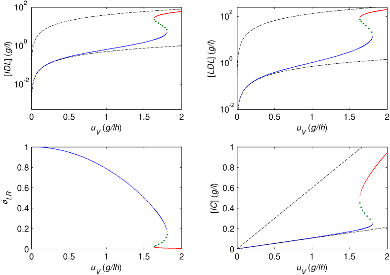
Figure 2: Plot of equilibrium solutions versus $u_{V}$. We show stable solutions (solid lines), unstable solutions (dotted lines), and bounds (6)–(9) (dashed lines) as a function of $u_{V}$ with parameters: { $k_{V}=0.3h^{-1}$, $k_{I}=0.025h^{-1}$, $d_{I}=2h^{-1}$, $d_{L}=0.01h^{-1}$, $d=0.0075h^{-1}$, $\chi_{I}=0.1$, $\chi_{L}=0.6$, $b=0.1lg^{-1}$, $c=0.05g(lh)^{-1}$; $d_{IC}=1h^{-1}$ }. For this set of parameters the system shows bistability. The bifurcations, obtained through (14), occur at: $u_{V,\text{bif}}\approx 1.637$ and $u_{V,\text{bif}}\approx 1.811$. The approximation (16) to the latter is 1.759.

We numerically explore the fixed point equation (10) and record how the number and stability of positive fixed points change as the control parameters are varied. Figure 2 shows a numerical bifurcation diagram as a function of $u_{V}$, for a given set of parameters. The system has two distinct (sometimes coexisting) stable solutions: a low and a high cholesterol branch. For small (high) $u_{V}$, only the low (high) branch exists. For intermediate values of $u_{V}$, the two stable branches (high and low) and an unstable solution coexist. The existence of this coexistence region leads to the possibility of hysteresis and a delayed return to the normal state when $u_{V}$ is swept. The transitions that delimit the coexistence region are two saddle-node bifurcations. A similar bifurcation diagram (Figure 3), with equivalent saddle-node bifurcations, is obtained by sweeping the other control parameter $d_{IC}$, although in this case the transition to a higher cholesterol state is produced by decreasing $d_{IC}$. These bifurcations could be of physiological relevance because the parameters $u_{V}$ and $d_{IC}$ can be regulated through diet and medication.

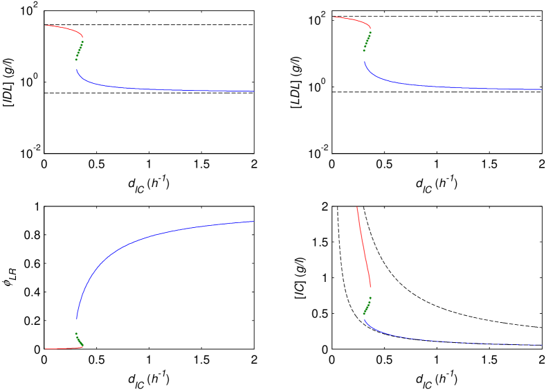
Figure 3: Equilibrium solutions versus $d_{IC}$. We show stable solutions (solid lines), unstable solutions (dotted lines), and bounds (dashed lines) as a function of $d_{IC}$. All parameters as in Fig. 2 and $u_{V}=1\,g(lh)^{-1}$. The bifurcations for this set of parameters, obtained through (14), occur at: $d_{IC,\text{bif}}\approx 0.373$ and $d_{IC,\text{bif}}\approx 0.305$. The approximation (16) to the latter is 0.323.

The nature of the bifurcation diagram depends on the non-control parameters of the model. In fact, the coexistence region does not exist in certain regions of parameter space. In that case, the transition from the low to the high cholesterol solution is smooth, without undergoing a bifurcation (i.e., no sudden jumps and no hysteresis). We make this more precise by analysing the equation for the bifurcation points. Rewrite the fixed point equation (10) as:

$$(y-1)(y+g)(y+f)^{2}+Z\,y\,(y+hf)(y+f+g)=0$$ (12)

where $y={\phi_{LR}}_{eq}$ and the following ratios of parameters have been defined:

$$e=b/c,\,f=k_{I}/d_{I},\,g=d/d_{L},\,h=\chi_{L}/\chi_{I},\,Z=u_{V}^{2}\,e\,\chi_{I}/d_{IC}.$$ (13)

The bifurcation points are the solutions of an augmented system of equations, formed by the fixed point equation and the condition that the Jacobian of (1)–(5) vanishes. Using Groebner bases (or considerations about monotonicity and curvature of (12)) we obtain a quintic polynomial equation for the bifurcation points $y_{\text{bif}}$:

$$y_{\text{bif}}^{5}+(2\,g+2\,f\,h+f)\,y_{\text{bif}}^{4}+(g^{2}+3\,f^{2}\,h+f-f\,h-g\,f+4\,f\,h\,g)\,y_{\text{bif}}^{3}\\ \mbox{}+(4\,g\,f+f^{2}-f^{2}\,g+f^{3}\,h-2\,f\,h\,g+2\,f^{2}\,h\,g-g^{2}\,f-f^{2}\,h+2\,f\,h\,g^{2})\,y_{\text{bif}}^{2}\\ \mbox{}+(2\,f^{2}\,g-f\,h\,g^{2}+2\,g^{2}\,f+f^{2}\,h\,g)\,y_{\text{bif}}+f^{3}\,h\,g+f^{2}\,h\,g^{2}=0.$$ (14)

Based on Descartes’ rule, we conclude that there is no coexistence region (and no bifurcations) if:

$$g^{2}+3\,f^{2}\,h+f-f\,h-g\,f+4\,f\,h\,g >0$$

$$4\,g\,f+f^{2}-f^{2}\,g+f^{3}\,h-2\,f\,h\,g+2\,f^{2}\,h\,g-g^{2}\,f-f^{2}\,h+2\,f\,h\,g^{2} >0$$

$$2\,f^{2}\,g-f\,h\,g^{2}+2\,g^{2}\,f+f^{2}\,h\,g >0.$$

These inequalities can be tested for each set of parameters to establish a sufficient condition for the saddle-node bifurcations to exist.

Further insight can be gathered through explicit approximate formulas for the bifurcations. Consider the limit case with $d=0$, i.e., when there is no direct uptake of cholesterol by the cell and only receptor-mediated intake is possible. In this case, the fixed point equation (12) simplifies to:

$$y\,(y+f)\,\left(y^{2}+(f-1+Z)y+f(Zh-1)\right)=0,$$

leading to the following bifurcation points for this limit case:

$$4f(Zh-1) =0 \Rightarrow u_{V,\text{bif}}^{*} =\sqrt{\frac{d_{IC}}{e\chi_{I}\,h}}$$ (15)

$$\frac{(f-1+Z)^{2}}{f(Zh-1)} =4 \Rightarrow u_{V,\text{bif}}^{*} =\sqrt{\frac{d_{IC}}{e\chi_{I}}\left(1-f+2fh-2\sqrt{f(h-1)(fh+1)}\right)}.$$ (16)

Eq. (16) marks the point above which the low cholesterol branch ceases to exist and serves as a good approximation for the bifurcation of the full model if $d$ is small. The approximate formulas (15)–(16) explain the overall dependence on $u_{V}$ and $d_{IC}$ of the bifurcation points shown in Figs. 2 and 3.

3.2 Sensitivity Analysis of the Equilibrium Solution

In order to ascertain how variations in parameter values (e.g., among individuals or due to age) affect the results, we perform a sensitivity analysis of the system. Because of its physiological relevance, we focus on the variability of the low cholesterol branch under parameter uncertainty.

Parameter	Variable	Sensitivity over lower branch ($u_{V}\leq u_{V,\text{max}}$)
		Median	Range
$k_{I}\in[0.025,0.1]$	$[IDL]$	0.027	$[0.0038,0.036]$
($u_{V,\text{max}}=1.1$)	$[LDL]$	1.18	$[1.16,1.26]$
	$\phi_{LR}$	0.013	$[3.1\times 10^{-4},0.074]$
	$[IC]$	0.17	$[0.15,0.21]$
$d_{I}\in[0.5,2]$	$[IDL]$	1.83	$[1.79,2.23]$
($u_{V,\text{max}}=1.4$)	$[LDL]$	1.85	$[1.79,2.48]$
	$\phi_{LR}$	0.023	$[3.1\times 10^{-4},0.22]$
	$[IC]$	0.18	$[0.16,0.34]$
$d_{L}\in[0.005,0.02]$	$[IDL]$	$5.3\times 10^{-4}$	$[8.5\times 10^{-6},0.0038]$
($u_{V,\text{max}}=1.3$)	$[LDL]$	$0.82$	$[0.67,0.87]$
	$\phi_{LR}$	$5.4\times 10^{-4}$	$[8.6\times 10^{-6},0.0039]$
	$[IC]$	$3.4\times 10^{-5}$	$[5.0\times 10^{-7},3.4\times 10^{-4}]$
$d\in[0.0025,0.0075]$	$[IDL]$	$4.6\times 10^{-4}$	$[5.9\times 10^{-6},0.0045]$
($u_{V,\text{max}}=1.4$)	$[LDL]$	0.38	$[0.34,0.50$]
	$\phi_{LR}$	$4.7\times 10^{-4}$	$[6.0\times 10^{-6},0.0046]$
	$[IC]$	$3.0\times 10^{-5}$	$[3.5\times 10^{-7},4.3\times 10^{-4}]$
$e=b/c\in[0.25,2.5]$	$[IDL]$	0.15	$[0.0024,0.80]$
($u_{V,\text{max}}=1.4$)	$[LDL]$	0.23	$[0.0037,1.23]$
	$\phi_{LR}$	0.15	$[0.0024,0.70]$
	$[IC]$	0.0093	$[1.4\times 10^{-4},0.064]$
$\chi_{I}\in[0.25,0.45]$	$[IDL]$	0.12	$[0.0039,0.76]$
($u_{V,\text{max}}=0.9$)	$[LDL]$	0.18	$[0.0062,1.06]$
	$\phi_{LR}$	0.12	$[0.004,0.71]$
	$[IC]$	0.56	$[0.56,0.56]$
$\chi_{L}\in[0.4,0.5]$	$[IDL]$	0.0018	$[2.4\times 10^{-5},0.014]$
($u_{V,\text{max}}=1.4$)	$[LDL]$	$0.0027$	$[3.8\times 10^{-5},0.21]$
	$\phi_{LR}$	$0.0018$	$[2.5\times 10^{-5},0.015]$
	$[IC]$	$0.013$	$[0.012,0.021]$

Table 3: Sensitivity of the variables of the model on the lower branch to variation of parameters one at a time. The sensitivity is calculated as the range divided by the median of each variable for five different values of the parameter that appears in the first column. The third and fourth columns report the median sensitivity and the range of calculated sensitivities over the lower branch (up to the value $u_{V,\text{max}}$). The salient feature of the analysis is the high sensitivity of $[LDL]$ to all parameters and the relative insensitivity of $[IC]$ to almost all parameters.

Table 3 summarises the sensitivity of the low cholesterol branch when parameters are modified one at a time. Consider for instance the effect of $d$, which parameterises the non-specific uptake of LDL. We have calculated numerical bifurcation diagrams similar to those in Figure 2 for values of $d\in[0.0025,0.0075]$. As $d$ is varied, the values of the lower and upper branches and the location of the bifurcations change. However, as expected from (6)–(9), only the $[LDL]$ is affected significantly. To make this more precise, we calculate the sensitivity for each variable over the lower branch ($u_{V}\leq 1.4\,g(lh)^{-1}$) by obtaining the average ratio of the range and median of the equilibrium values. Clearly, $[LDL]$ has the highest sensitivity to $d$. The sensitivity to other parameters is summarised in Table 3: $d_{L}$ virtually only affects $[LDL]$, as indicated by (6)–(9); variations of $e=b/c$ displace the bifurcation point (16), but $[IC]$ is fairly insensitive; variations in $k_{I}$ and $d_{I}$ have a large effect on $[LDL]$, but only $d_{I}$ affects $[IDL]$; the sensitivity of $[IC]$ to $\chi_{I}$ is moderate as compared to the sensitivity of $[LDL]$ or $[IDL]$ to $k_{I}$ and $d_{I}$.

We have also performed a Monte Carlo sensitivity analysis with respect to variations of all parameters at once by sampling and averaging over the uniform hypercube of non-control parameters in Table 3. The results show that the median sensitivity of $[LDL]$ to global parametric variations is an order of magnitude larger than that of $[IC]$ over the low cholesterol branch. The conclusion of the sensitivity analysis is that while the plasma cholesterol $[LDL]$ is sensitive to most parameters, the intracellular cholesterol $[IC]$ is robust to parameter perturbations. In essence, this is a system where $[IC]$ is tightly controlled whereas $[LDL]$ (the variable measured medically) is poorly controlled and can undergo wide variations.

Based on experimental observations (Goldstein and Brown, 1977), we have modelled the regulation of the nuclear synthesis of LDL receptors as a simple reciprocal feedback. However, the qualitative features of the system are robust to our choice of functional form. The regulation term in Eq. (4) is a particular case of the standard inhibiting feedback (Murray, 1990): $c(1-\phi_{LR})/(q+[IC]^{n})$, with $n=1$ and $q\ll[IC]$. Note, however, that the presence of $q$ and $n$ does not change the bounds (6)–(9). Therefore, the low and high cholesterol asymptotic regimes and the asymptotic response of the system to time-varying inputs (Section 4.2) remain unchanged. We have also checked numerically that the system still undergoes transitions between low and high cholesterol states; $q$ and $n$ have the effect of displacing the bifurcation points and modifying the extent of the coexistence region. In general, for large $q$ the effect of the feedback is reduced, thus making the transition to the high cholesterol branch easier; for $n>1$ the feedback is more efficient, thus enlarging the region of existence of the lower cholesterol branch.

4 Physiological Implications of the Model

4.1 Parametric Effects of Medical and Genetic Conditions

4.1.1 Tangier Disease and Reverse Cholesterol Transport

Tangier disease is a deadly disease in which vanishing reverse cholesterol transport leads to accumulation of cholesterol in all cells (Young and Fielding, 1999). In our model, the parameter $d_{IC}$ depends directly on reverse cholesterol transport. Note that only the bounds on $[IC]_{eq}$ are inversely proportional to $d_{IC}$. This means that low values of $d_{IC}$ lead to diverging levels of intracellular cholesterol, while the plasma cholesterol levels saturate (Fig. 3).

4.1.2 Lipase Enzyme Activity

In a review article, Stein and Stein (2003) report that reduced enzyme activity can lead to reduced plasma cholesterol concentrations in mice and rabbits. Similar results might hold for humans. A conclusion of our sensitivity analysis (Table 3) is that variations in $k_{I}$ produce sharp changes in $[LDL]$ without affecting the other variables significantly. Further numerics (not shown) show that decreasing $k_{I}$ decreases $[LDL]$.

4.1.3 Familial Hypercholesterolemia

Familial hypercholesterolemia (FH) is a genetic disease caused by mutations in the LDL receptor gene (Goldstein and Brown, 1977; Hobbs et al., 1990). In the heterozygous case of FH, which affects about 1 in 500 people in generic populations and even higher ratios in more inclusive populations, cells express around half the normal number of functional receptors on their surface leading to a two-fold increase in $[LDL]$. The homozygous case is much more rare (about 1 per million) but more severe. In this case, a negligible amount of functional LDL receptors lead to a dramatic rise of LDL plasma levels. These diseased individuals frequently dye of myocardial infarction or stroke in their teens. Table 4 presents a classification of FH gene mutations with their physiological implications (Hobbs et al., 1990). We also show how the mutations can be represented in terms of the parameters of our model.

Mutation Class	Physiological effect	Affected Parameter
1	Reduced synthesis of LR	$c\downarrow$
2	Reduced transport of LR
3	Reduced binding of IDL/LDL to LR	$d_{I}\downarrow$ and/or $d_{L}\downarrow$
4	Reduced number of LR in coated pits
5	Diminished recycling of LR	$b\uparrow$

Table 4: Gene mutations that lead to familial hypercholesterolemia. Mutations leading to FH as classified by Hobbs et al. (1990) and how they affect the parameters of the model.

Most of the medical observations in Hobbs et al. (1990) refer to mutation classes 3 and 4, both hetero- and homozygous. In terms of our model, heterozygous mutations 3 and 4 would halve $d_{I}$ and $d_{L}$. This produces roughly a two-fold (up to four-fold) increase in $[LDL]$, as deduced from the lower bound in (7) and Table 2. One of the homozygous mutations blocks the binding of both IDL and LDL to LR, hence $d_{I}=d_{L}=0$. Again from (7), this would increase $[LDL]$ by a factor $(1+d_{L}/d)(1+d_{I}/k_{I})$, which is roughly 10-fold (and up to several hundred times-fold). These numerical factors correspond well to those in the literature (Hobbs et al., 1990). Under another homozygous mutation 3 and 4, LDL receptors bind to IDL but not to LDL, i.e., $d_{L}=0$. This produces an increase of $[LDL]$ in the lower branch by a factor of $(1+d_{L}/d)$, which is two-fold (up to nine-fold) but still an order of magnitude smaller than that of the other homozygous case. Moreover, the characteristic time scale for the catabolism of LDL (see Section 4.2) increases from $(d+d_{L})^{-1}$ (around two days) to $d^{-1}$ (over a week). Again, this coincides with experimental observations that the removal of LDL from the plasma is delayed and the increase in plasma LDL is moderate (Hobbs et al., 1990).

Medical evidence for mutations 1-2 and 5 is scarcely reported. In our model, they would translate into an increase of $e=b/c$ which would have a small effect on the plasma concentrations on the lower cholesterol branch. However, as seen in Eqs. (15) and (16), an increase in $e$ would lower the bifurcation point, making it easier to jump to the high cholesterol branch in response to an increase in $u_{V}$ or a decrease in $d_{IC}$. Therefore, under these mutations the parameter region where the lower cholesterol regime exists would be reduced.

Other observations in Hobbs et al. (1990) could also be interpreted in terms of our model. For example, it was reported that despite treatment with statins and lipid-lowering medications, the plasma cholesterol of some patients remained between 600 and $1200\,mg/dl$, five to ten times the normal levels. As seen in Figs. 2 and 3 and discussed further in Section 4.2.1, the presence of bistability means that once on the upper branch it is more difficult to return to the low cholesterol state by reducing $u_{V}$, e.g. through statin medication. Another intriguing observation is the dramatic clinical variability among FH patients with the same genetic mutation. A possible explanation is the robustness of $[IC]_{eq}$ to variations in the physiological parameters. Indeed, from the lower bound in (9) we estimate that $[IC]$ would only increase by 1.1 to 1.5 times under homozygotic FH, while the corresponding increase in $[LDL]$ would range from one to almost three orders of magnitude. This would allow the development of individuals who would have similar levels of intracellular cholesterol while the LDL plasma levels could be very high in some cases, with different clinical consequences.

4.2 Response to Time-dependent Inputs

The time scales of the system span from a few hours up to a week. These time scales govern the way in which the system responds to external drives or perturbations to the variables. To clarify their dynamical role, we use singular perturbation methods to obtain slow and fast manifolds (Khalil, 2000) relevant to the system. We have seen previously that the lower bound ($\phi_{LR}=1$) and upper bound ($\phi_{LR}=0$) are approached asymptotically as $u_{V}\to 0$ and as $u_{V}\to\infty$, respectively. In these singular asymptotic limits, the system (1)–(5) reduces to a linear system of the form:

$$\frac{d\mathbf{x}}{dt}=A_{k}\,\mathbf{x}+\mathbf{b},\quad k=\{l,u\},$$ (17)

where $\mathbf{x}=[[VLDL]\ [IDL]\ [LDL]\ [IC]]^{\mathrm{T}},\quad\mathbf{b}=[u_{V}\ 0\ 0\ 0]^{\mathrm{T}}$,

$$A_{l}=\left[\begin{array}[]{cccc}-k_{V}&0&0&0\\ k_{V}&-k_{I}-d_{I}&0&0\\ 0&k_{I}&-d_{L}-d&0\\ 0&\chi_{I}d_{I}&\chi_{L}(d_{L}+d)&-d_{IC}\\ \end{array}\right],\,\ A_{u}=\left[\begin{array}[]{cccc}-k_{V}&0&0&0\\ k_{V}&-k_{I}&0&0\\ 0&k_{I}&-d&0\\ 0&0&\chi_{L}d&-d_{IC}\\ \end{array}\right],$$

and $l,u$ denote lower and upper asymptotic regimes, respectively. The inverse of the matrix eigenvalues are the characteristic times for each variable to return to equilibrium:

$$\left(k_{I}+d_{I}\right)^{-1}\approx 0.5<d_{IC}^{-1}\approx 1\,h<k_{V}^{-1}\approx 10\\ <k_{I}^{-1}\approx 40<\left(d+d_{L}\right)^{-1}\approx 70<d^{-1}\approx 200,$$ (18)

all of them given in hours. Note that the slowest time scale increases from $(d+d_{L})^{-1}$ (on the scale of a day) on the lower branch to $d^{-1}$ (over one week) on the upper branch.

4.2.1 Response to slow drifts in the control parameters

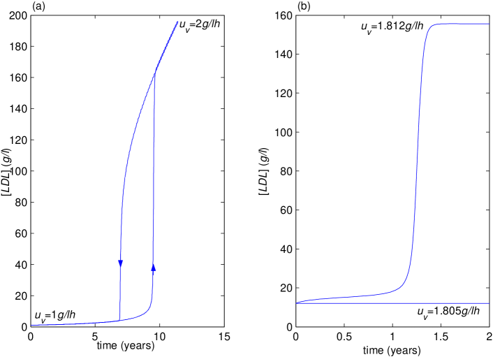
Figure 4: Quasi-static nonlinear effects (a) Hysteresis curve obtained when $u_{V}$ is increased by $0.01\,g(lh)^{-1}$ every 1000 hours from $u_{V}=1\,g(lh)^{-1}$ to $u_{V}=2\,g(lh)^{-1}$, and then decreased at the same rate to its initial value. (b) Bottleneck dynamics caused by the ‘ghost’ saddle-node around the bifurcation. The jump to the upper branch occurs a year after a small, but permanent, perturbation of $u_{V}$ has occurred.

The response of the system to a slowly drifting input $u_{V}(t)$, which varies on a time scale slower than $d^{-1}$, will be quasi-static, tracking the equilibrium points. This can reveal nonlinear behaviour, such as hysteresis and bottleneck phenomena (Strogatz, 1994), which can have physiological ramifications.

If the system is in a parametric region where it can undergo bifurcations (as in Figs. 2 and 3), it will exhibit standard hysteresis when $u_{V}$ is swept continuously from the lower branch to the upper branch and backwards (Figure 4a). This means that once in the upper branch it is more difficult to return to the low cholesterol state by reducing $u_{V}$ (e.g., through statin medication).

Another effect of the existence of saddle-node bifurcations is the possibility of bottleneck dynamics caused by saddle-node ghosts. This can translate into long-lived transients when the system is parametrically close to the bifurcation points. Figure 4b shows the time evolution of the system for two values of $u_{V}$, one below and one above (but very close) to the bifurcation. The former remains in the low cholesterol branch and the latter jumps the high cholesterol solution. However, although the actual transition is relatively sudden (on the order of a week, $d^{-1}$), it occurs after a prolonged period of more than a year in which the system behaves as if in the (no longer existing) low cholesterol state. This pseudo-steady (ghost) behaviour would make it difficult to detect a very slow $u_{V}$ drift, which can suddenly lead to high plasma cholesterol values, if clinical measurements are infrequent.

4.2.2 Response to periodic inputs

Figure 5: Forced oscillations with a period of one day. Response of $[IDL]$, $[LDL]$ and $[IC]$ to a periodic forcing $u_{V}=U_{V}\,\left(1+\sin(\omega\,t)\right)$ with $\omega=2\pi/24\,h^{-1}$ for values of $U_{V}=$ 1.25 (solid line), 1.75 (dashed line), 2.25 (dot-dashed line). All other parameters as in Fig. 2. The variables of the system exhibit different dynamical responses at this forcing frequency. The variability of $[IC]$ is linked to that of $[IDL]$ on the lower branch and to that of $[LDL]$ on the upper branch.

We study now the physiological implications of the response of the system to forced input oscillations with periods of days up to months. It is reasonable to assume that the production of VLDL ($u_{V}(t)$) can have a strong periodic content on the order of a day since VLDL is produced at increased levels during the night; dietary intake is often highly cyclic; and the ingestion of statins to lower $u_{V}$ generally follows a daily cycle. As expected, entrainment phenomena can be observed in Figure 5, where we show the response of the system to forced oscillations with period of one day and increasing amplitude and mean. $[LDL]$ is relatively insensitive to the oscillatory drive, while $[IDL]$ exhibits large oscillatory amplitudes both for small and large drives. However, the salient feature is the different amplitude of the response of $[IC]$ in both regimes. Qualitatively, this can be understood from the fact that $[IC]$ changes from being tightly linked to $[IDL]$ at low drives, when the amount of LDL receptors is high, to being governed by $[LDL]$ on the upper branch, where the low $\phi_{LR}$ makes IDL endocytosis virtually impossible while LDL can still be absorbed through the non-receptor mediated route.

A quantitative understanding of the responses in Figure 5 emerges from a more detailed analysis. If we consider a periodic input

$$u_{V}(t)=U_{V}\left(1+P\sin(\omega\,t)\right),$$ (19)

it follows that the time response of the asymptotic system (17) is sinusoidal of the form

$$x_{i}=x_{i,av}+x_{i,s}\sin(\omega\,t)+x_{i,c}\cos(\omega\,t),\qquad i=1,\ldots,4,$$ (20)

with average $x_{i,av}$ and amplitude $x_{i,amp}=\sqrt{x_{i,s}^{2}+x_{i,c}^{2}}$. We have calculated the sinusoidal responses for $[IDL],[LDL]$ and $[IC]$ on both branches. On the lower branch we get:

$$[IDL]_{av,l} =\frac{U_{V}}{k_{I}+d_{I}},\quad\frac{[IDL]_{amp,l}}{[IDL]_{av,l}}=\frac{P}{\sqrt{\left(1+\left(\frac{\omega}{k_{V}}\right)^{2}\right)\,\left(1+\left(\frac{\omega}{k_{I}+d_{I}}\right)^{2}\right)}}$$ (21)

$$[LDL]_{av,l} =\frac{k_{I}\,U_{V}}{\left(k_{I}+d_{I}\right)\left(d+d_{L}\right)},\quad\frac{[LDL]_{amp,l}}{[LDL]_{av,l}}=\frac{[IDL]_{amp,l}}{[IDL]_{av,l}}\frac{1}{\sqrt{1+\left(\frac{\omega}{d+d_{L}}\right)^{2}}}$$ (22)

$$[IC]_{av,l} =\frac{(\chi_{I}d_{I}+\chi_{L}k_{I})\,U_{V}}{\left(k_{I}+d_{I}\right)d_{IC}},$$

$$\frac{[IC]_{amp,l}}{[IC]_{av,l}}=\frac{[IDL]_{amp,l}}{[IDL]_{av,l}}\sqrt{\frac{1+\left(\frac{\omega}{d+d_{L}}\,\frac{\chi_{I}d_{I}}{\chi_{I}d_{I}+\chi_{L}k_{I}}\right)^{2}}{\left(1+\left(\frac{\omega}{d+d_{L}}\right)^{2}\right)\,\left(1+\left(\frac{\omega}{d_{IC}}\right)^{2}\right)}},$$ (23)

while on the upper branch we obtain:

$$[IDL]_{av,u} =\frac{U_{V}}{k_{I}}, \frac{[IDL]_{amp,u}}{[IDL]_{av,u}} =\frac{P}{\sqrt{\left(1+\left(\frac{\omega}{k_{V}}\right)^{2}\right)\left(1+\left(\frac{\omega}{k_{I}}\right)^{2}\right)}}$$ (24)

$$[LDL]_{av,u} =\frac{U_{V}}{d}, \frac{[LDL]_{amp,u}}{[LDL]_{av,u}} =\frac{[IDL]_{amp,u}}{[IDL]_{av,u}}\frac{1}{\sqrt{1+\left(\frac{\omega}{d}\right)^{2}}}$$ (25)

$$[IC]_{av,u} =\frac{\chi_{L}U_{V}}{d_{IC}}, \frac{[IC]_{amp,u}}{[IC]_{av,u}} =\frac{[LDL]_{amp,u}}{[LDL]_{av,u}}\frac{1}{\sqrt{1+\left(\frac{\omega}{d_{IC}}\right)^{2}}}.$$ (26)

The sinusoidal solutions (20)–(26), which are valid asymptotically in the limits $u_{V}\to 0$ (lower) and $u_{V}\to\infty$ (upper), provide a good approximation when $U_{V}$ is either small or large. Clearly, one does not expect a pure sinusoidal response at intermediate values of $U_{V}$, as can be observed in Figure 5.

The change in the variability of $[IC]$ on both branches can now be traced to Eqs. (21)–(26). For a forcing period of one day ($\omega=\pi/12\approx 0.26\,h^{-1}$) and using the time scales (18), the key terms are $\omega/(d+d_{L})$ and $\omega/d$. Note how on the lower branch (23), the $\omega/(d+d_{L})$ terms cancel, with the effect that the relative variability $[IC]_{amp,l}/[IC]_{av,l}$ is tied to that of $[IDL]$. Onn the upper branch (26), $\omega/d_{IC}\ll 1$, which implies that the relative variability $[IC]_{amp,u}/[IC]_{av,u}$ is linked to that of $[LDL]$.

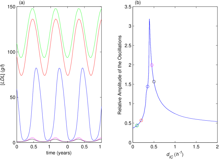
Figure 6: Forced oscillations with a period of 100 days. (a) Response of $[LDL]$ to a periodic forcing $u_{V}=\left(1+0.2\,\sin(\omega\,t)\right)$ with $\omega=2\pi/2400\,h^{-1}$ for values of $d_{IC}=[0.1,0.2,0.35,0.45,0.5]$, from top to bottom. All other parameters as in Fig. 3. As $d_{IC}$ increases, the system moves from the upper to the lower branch and the average level of $[LDL]$ decreases. (b) Relative amplitude of the oscillations, calculated as the ratio of range and mean of the oscillations from numerical simulations. The circles correspond to the values of $d_{IC}$ in (a). Note that the relative amplitude is similar in both asymptotic regimes. This can be understood from Eqs. (22) and (25), whence we obtain the relative amplitude to be $\approx 0.38$ (as $d_{IC}\to 0$) and $\approx 0.40$ (as $d_{IC}\to\infty$). The relative amplitude reaches a maximum close to the bifurcation, where the system jumps between the upper and lower branches and is at its most nonlinear. As an indication, the bifurcation for these parameters and $u_{V}=1$ occurs at $d_{IC}\approx 0.373$, close to the observed peak.

These observations suggest that the correlation between intracellular and plasma cholesterol concentrations could be used as a marker to detect the high cholesterol state. This effect would be most pronounced in hepatic cells but might still be observable in other cells and detectable through a skin test. (This would depend on how much IDL can penetrate peripheral cells by leaking through the capillary endothelium into the interstitial fluid.) A less practical alternative would imply repeated time measurements of $[IDL]$ to check for large amplitude oscillations.

We have also explored the response of the system to oscillations with lower frequency, as would be induced by seasonal cycles. Figure 6 shows the response of $[LDL]$ to oscillatory inputs with period of 100 days at different values of $d_{IC}$ as shown in Fig. 3. Consistent with Eqs. (22) and (25), the average level of $[LDL]$ on the upper branch is high, of order $\sim d^{-1}\approx 133$, while on the lower branch it is much smaller, of order $\sim k_{I}d_{I}^{-1}(d+d_{L})^{-1}\approx 0.7$. However, the relative amplitude of the oscillations of $[LDL]$ in both asymptotic regimes is of the same order. It is precisely at the bifurcation point, when the system oscillates between the low and high cholesterol regimes, that the oscillations are larger in relative terms (Figure 6). This could be used to characterise the system if sufficiently frequent measurements are available.

5 Discussion

Understanding lipoprotein metabolism is important because high lipoprotein concentration in the plasma is a major risk factor for atherosclerosis, the most common cause of death in Western societies. We have introduced a dynamical model of lipoprotein metabolism derived by combining physiological cascading and cellular processes. The model goes beyond compartmental models in that we have included both the nonlinear absorption of IDL and LDL by cells, and a feedback mechanism by which the cell regulates the number of its LDL receptors based on the concentration of intracellular cholesterol IC.

This low-dimensional, nonlinear model shows bistability and hysteresis between a low and a high cholesterol state. Our bifurcation analysis of the key control parameters ($u_{V}$ and $d_{IC}$) can be related to physiologically meaningful processes: diet and statin medication in the case of $u_{V}$; reverse cholesterol transport through HDL in the case of $d_{IC}$. We have checked that the observed behaviour is relatively robust with respect to all other parameters. An important outcome of our sensitivity analysis is that the most robust feature in the low cholesterol state is the concentration of intracellular cholesterol $[IC]$, while the plasma concentrations $[IDL]$ and $[LDL]$ can vary widely. This indicates that plasma cholesterol is not a tightly controlled variable in the system, implying that very different values of plasma $[LDL]$ can be compatible with viable cellular function. It is conceivable, however, that the high levels of $[LDL]$, innocuous at the cellular level, could lead to the initiation of disease-linked processes at the physiological level.

We have also obtained estimates for the characteristic time scales governing the dynamics of the model in the low and high cholesterol states. These time scales account for the dynamical responses of the system to forced input oscillations with very different periods. The model shows dynamical behaviour which could be used to diagnose the state of the system if repeated measurements of plasma and/or cellular cholesterol with the correct timing and periodicity are performed, as indicated by Figs. 5 and 6. If measurements are too sparse, the onset of permanent high cholesterol levels might go undetected, with the possibility of a difficult return to lower levels due to hysteretic effects. Measurements taken periodically on the order of hours or months could provide complementary clues to the state of the system. If we assume that periodic inputs to the system are important, measuring the relative variability of LDL and cellular cholesterol (possibly through skin tests) could lead to markers for the detection of the intrinsic regime of the system.

Our dynamical model is directly derived from the underlying physiological and cellular processes. However, some of our approximations are crude and several directions for improvement could be pursued. The level of the plasma cholesterol on the high cholesterol branch ($[VLDL]_{eq}+[IDL]_{eq}+[LDL]_{eq}$) is unphysiologically high in the current model. This suggests the presence of other physiological mechanisms of elimination that have not been included in the model. Another extension would include time delays (Dugard and Verriest, 1998) to account for mass transfer (e.g., the delayed intake of IDL and LDL via LR-mediated endocytosis) and control mechanisms (e.g., the delayed genetic regulatory loop in the synthesis of LR). Furthermore, the model could be extended to include explicitly the regulatory and synthetic pathways involving the intracellular LDL receptors. It would also be important to distinguish between hepatic and non-hepatic cells, as hepatic cells play a more central role in lipoprotein metabolism. In particular, the rate of lipoprotein uptake in liver cells is different; increased uptake of LDL in liver cells lowers the production rate of VLDL (i.e., $u_{V}$) through an additional regulating feedback; and statins reduce the inhibiting effect of $[IC]$ on the synthesis of LR in liver cells only.

Especially important would be to extend our description of reverse cholesterol transport to include $[HDL]$ explicitly as a variable. Indeed, $20\%$ of the total plasma cholesterol in healthy individuals ($40\,mg/dl$) is carried by HDL. Our preliminary work in this direction indicates that the number of nonnegative equilibria remains unchanged in the enlarged system that includes $[HDL]$, and the qualitative features of the system should hold. Because the relationship between plasma $[LDL]$ and $[HDL]$ is of major importance in clinical trials, this would be a crucial element to enhance the applicability of the model.

Further modelling of lipoprotein metabolism could bring light to several open questions. To name but a few, it is still unknown why the plasma cholesterol concentrations in adult humans are so unnecessarily high (Goldstein and Brown, 1977); what the exact effects of statins in the metabolic system are (Davidson and Jacobson, 2001); and which of the processes could be best targeted to reduce plasma LDL concentrations.

Appendices

Appendix A Derivation of the feedback term

The feedback term in Eq. (4) follows from a more detailed (but still simplified) derivation that includes the three compartments of intra-cellular LDL receptors (complexed, recycled, nucleus-synthesised) as shown in Figure 7. The kinetic rate equations are:

$$\frac{d[LR_{comp}]}{dt} =\beta\alpha\left(d_{I}[IDL]+d_{L}[LDL]\right)\phi_{LR}-\epsilon[LR_{comp}]$$ (27)

$$\frac{d[LR_{rec}]}{dt} =\epsilon(1-\gamma)[LR_{comp}]-\delta[LR_{rec}]\left(1-\phi_{LR}\right)$$ (28)

$$\frac{d[LR_{nuc}]}{dt} =\frac{c_{1}}{[IC]}-k[LR_{nuc}]-\delta[LR_{nuc}]\left(1-\phi_{LR}\right)$$ (29)

$$\frac{d\phi_{LR}}{dt} =-\alpha\left(d_{I}[IDL]+d_{L}[LDL]\right)\phi_{LR}+\frac{\delta}{\beta}([LR_{rec}]+[LR_{nuc}])\left(1-\phi_{LR}\right).$$ (30)

If we assume steady-state conditions: $\frac{d[LR_{comp}]}{dt}=\frac{d[LR_{rec}]}{dt}=\frac{d[LR_{nuc}]}{dt}=0$, and that $k\gg\delta$, then Eq. (4) follows with $b=\alpha\gamma$ and $c=\delta c_{1}/\beta k$.

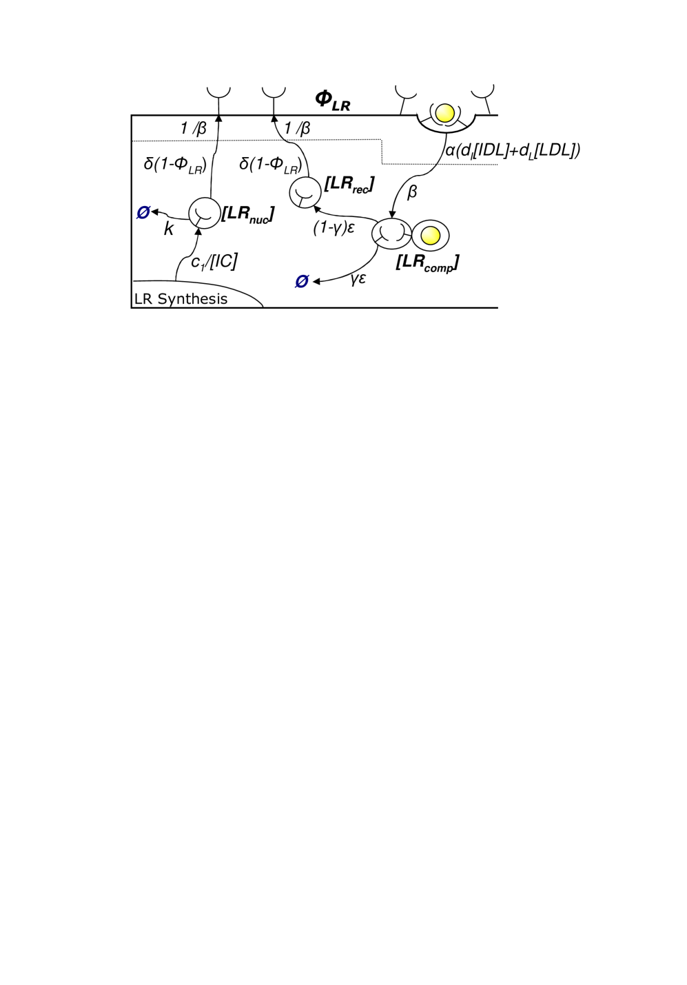
Figure 7: Schematic description of the feedback term. An expanded view of the portion of Figure 1 that is related to the processes involved in the synthesis and recycling of LDL receptors inside the cell. If we assume steady state for the intracellular LR compartments, and that the turnover of nucleus-synthesised LR ($k$) is large compared to the probability of its insertion into the membrane ($\delta$), these processes lead to Equation (4). The factor $\beta$ performs the appropriate dimensional conversions to account for the fact that $\phi_{LR}$ is a non-dimensional surface occupancy fraction. Note also that $\gamma$ is the fraction of non-recycled LDL receptors. All the other constants are rate constants with the appropriate units.

References

- Adiels (2002) Adiels, M., 2002. A Compartmental Model for Kinetics of Apolipoprotein B-100 and Triglycerides in VLDL1 and VLDL2 in Normolipidemic Subjects. Master’s thesis, Chalmers University of Technology.
- Bywater et al. (2002) Bywater, R. P., Sorensen, A., Rogen, P., Hjorth, P. G., 2002. Construction of the Simplest Model to Explain Complex Receptor Activation Kinetics. J. theor. Biol. 218, 139–147.
- Chopra and Thurnham (1999) Chopra, M., Thurnham, D. I., 1999. Antioxidants and lipoprotein metabolism. Proc. of the Nutrition Society 58, 663–671.
- Cobbold et al. (2002) Cobbold, C. A., Sherratt, J. A., Maxwell, S. R. J., 2002. Lipoprotein Oxidation and its Significance for Atherosclerosis: A Mathematical Approach. Bulletin of Mathematical Biology 64, 65–95.
- Converse and Skinner (1992) Converse, C. A., Skinner, E. R., 1992. Lipoprotein Analysis: A Practical Approach. IRL Press at Oxford University Press, New York.
- Cooper (2000) Cooper, G. M., 2000. The Cell (a molecular approach), Edition. ASM Press, Boston.
- Davidson and Jacobson (2001) Davidson, M. H., Jacobson, T. A., 2001. How Statins Work: The Development of Cardiovascular Disease and Its Treatment With 3-Hydroxy-3-Methylglutarylcoenzyme A Reductase Inhibitors. Cardiology Clinical Updates - ©2001 Medscape, Inc.
- Dietschy et al. (1978) Dietschy, J. M., Gotto, A. M., Ontko, J. A. (Eds.), 1978. Disturbances in Lipid and Lipoprotein Metabolism. American Physiological Society, Bethesda, Maryland.
- Dietschy et al. (1993) Dietschy, J. M., Turley, S. D., Spady, D. K., 1993. Role of liver in the maintenance of cholesterol and low density lipoprotein homeostasis in different animal species, including humans. Journal of Lipid Research 34, 1637–1659.
- Dugard and Verriest (1998) Dugard, L., Verriest, E. I., 1998. Stability and Control of Time-Delay Systems. Springer-Verlag, London, United Kingdom.
- Eisenfled and Grundy (1984) Eisenfled, J., Grundy, S. M., 1984. Extension of Compartmental Parameters to Blocks of Compartments with Application to Lipoprotein Kinetics. Mathematical Biosciences 68, 99–120.
- Glass and Witztum (2001) Glass, C. K., Witztum, J. L., 2001. Atherosclerosis: The Road Ahead. Cell 104, 503–516.