A domain wall model for spectral reflectance of plant leaves

Abstract

We model a plant leaf by using two-dimensional domain walls with internal structures. Such domain walls can be found as soliton solutions in field theory describing magnetic materials. The radiation scattered by such domain walls behaves quite similar to the spectral reflectance of plant leaves. The model nicely simulates the spectral reflectance of a plant leaf as a function of the wavelength.

I. Introduction. The study of the spectral behavior of vegetables is often used to investigate the characteristics of the electromagnetic radiation reflected by plant leaves, a plant as whole or a collection of plants. We should emphasize that the study of the spectral behavior in general means the study of spectral reflectance, spectral transmittance and spectral absorbance. Concerning the interaction of the solar energy with vegetables, the plant leaf plays a special role because it basically realizes the photosynthesis that is responsible by the formation of carbon compounds. The whole configuration of a plant leaf including form, position, structures, etc, adapts to receive in a most efficient way the solar beams, air and water which are necessary for realizing photosynthesis. Thus the knowledge of the properties of a plant leaf is clearly fundamental, especially in the study of the reflectance of a plant or even a culture of plants. Such predominance of the plant leaf is so important that the area of the other part of the plant in contact with the solar radiation is completely neglected 1 ; 1a . It is obvious, however, that the data obtained from a unique plant leaf cannot be used directly, without modifications, to a culture of plants. This is because there exist qualitative and quantitative differences between the aspects of unique plant leaf and a culture of plants in a field. The structures of the cells that constitute the three tissues of the leaves vary with the specie and ambient conditions. The compounds of the leaf that are of considerable importance in the study of interaction of a leaf with the radiation are: cellulose that are found in the cellular walls, solutes like ions and molecules, intercellular spaces and pigment inside chloroplasts such as carotene, xanthophyll and chlorophyll. The spectral behavior of a plant leaf is a function of its compounds, morphology and internal structure. Since the characteristics of the plant leaves are genetically controlled there exist differences in the spectral behavior among groups that are genetically distinct. The Fig. 1 shows possible paths of the radiation or incident energy over a plant leaf. A small amount of radiation is reflected from the cells around the surface of the plant leaf; the major part of the radiation is transmitted to the spongy mesophyll, where the cellular walls for incident angles sufficiently large reflect the incident radiation rays 2 . These multiple reflections are essentially a random process where the rays change their directions inside the plant leaf. Because the large number of cellular walls, some rays go back toward the source of radiation, while others are transmitted trough the plant leaf. The thickness of the plant leaf clearly affects the transmittance of the radiation, being larger than the reflectance for thin leaves. The opposite happens for thick leaves. The spectral response of a target, as a plant leaf considered in the present work, deal with the graphic representation of the reflectance in narrow and adjacent bands of wavelengths. This representation gives us the effect of the interaction of incident radiation and the target under investigation. Thus, the amplitude variations in spectral response give us clues about the spectral properties of the objects 3 ; 4 ; 7 ; 8 . The curve of reflectance of a plant leaf can be divided into ultraviolet region, visible region (400 - 700 nm), near infrared (700 - 1300 nm), and mid infrared (1300 - 2600 nm). However, the ultraviolet region usually is not considered because the most part of this radiation is scattered away and the vegetables does not make use of this radiation. The mid infrared is not considered here because of limitations on the sensor equipment in this region. The curve of reflectance obtained experimentally is shown in Fig. 2.

In this work, we model the plant leaf by a domain wall with internal structure 9 ; 10 ; 11 ; 12 ; 13 ; 14 . In the following section we show with details how this can be possible. The model is mainly based on the reflection probability that light neutral particles can suffer as they collide with such domain walls — in Ref. 9 this issue was initiated in another context. In our model the light neutral particles play the role of the electromagnetic radiation and the domain wall with internal structure plays the role of a plant leaf.

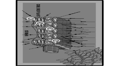
Figure 1: Transversal section of a plant leaf with possible paths of radiation rays. (1) upper epidermis, (2) palisade mesophyll, (3) spongy mesophyll and (4) lower epidermis.

The internal structures are small domain walls that we identify with the spaces among the spongy mesophyll. Domain walls are soliton solutions that appear in systems that exhibit spontaneous symmetry breaking, such as the Higgs mechanism applied in Particle Physics and the Ginzburg-Landau theory applied in Superconductivity. These systems usually present non-linearity into equations of motion. Such non-linearity is responsible for the formation of soliton solutions whose energy density is localized around a region of the space, and remains stable all times.

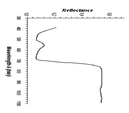
Figure 2: The spectral reflectance of a peanut leaf in the visible and infrared regions obtained experimentally.

II. The domain wall model. The dynamics of a system with two coupled real scalar fields $\phi$ and $\chi$ is described by a field theory with the Lagrangian

$${\cal L}=\frac{1}{2}\partial_{\mu}\phi\partial^{\mu}\phi+\frac{1}{2}\partial_{\mu}\chi\partial^{\mu}\chi-V(\phi,\chi).$$ (1)

Where the potential $V(\phi,\chi)$ belongs to a class of soliton models easily integrable 9 ; 10 ; 11 ; 12 ; 13 ; 14 given by

$$V=\frac{1}{2}\left(\frac{\partial W}{\partial\phi}\right)^{2}+\frac{1}{2}\left(\frac{\partial W}{\partial\phi}\right)^{2},$$ (2)

where $W$ is known as “superpotential” that for our purposes here it is sufficient to make the following choice

$$W=\nu\left(\frac{\phi^{3}}{3}-a^{2}\phi\right)+\mu\phi\chi^{2},$$ (3)

such that $V(\phi,\chi)$ can be written as

$$V(\phi,\chi) = \frac{1}{2}\nu^{2}(\phi^{2}-a^{2})^{2}+(2\mu^{2}+\nu\mu)\phi^{2}\chi^{2}-\nu\mu a^{2}\chi^{2}$$ (4)

$$+ \frac{1}{2}\mu^{2}\chi^{4}.$$

The scalar field $\phi$ describes the domain wall that we identify with a plant leaf. The scalar field $\chi$ describes the internal structures that appear as domain walls, which can form disk like structures 14 . These domain walls will be identified later with cellular walls inside the plant leaf. The meaning of the parameters $\nu$, $a$ and $\mu$ will become clear later. The field equation of motion are given by

$$\square\phi+\frac{\partial V}{\partial\phi}=0,$$ (5)

and

$$\square\chi+\frac{\partial V}{\partial\chi}=0.$$ (6)

Now we make use of perturbation theory, up to first order, around the soliton solutions $\bar{\phi}$ and $\bar{\chi}$ into the equations of motion (5) and (6), as $\chi=\bar{\chi}+\xi$ and $\phi=\bar{\phi}$, where $\xi$ represents the relevant fluctuations for the internal structures. Considering such fluctuations having the form $\xi=\xi(z)e^{-i(\omega t-k_{x}x-k_{y}y)}$ the relevant equation for the fluctuations reads

$$\partial_{z}^{2}\xi(z)+[-\omega^{2}+k_{x}^{2}+k_{y}^{2}]\xi(z)+\frac{\partial^{2}\overline{V}}{\partial\chi^{2}}\xi(z)=0,$$ (7)

which is a Schroedinger like equation. The bar means the function is evaluated at the original soliton solutions. By considering a domain wall approximately plane and static it suffices to work only with a spatial dimension such that the fields are functions as $\phi\equiv\phi(z)$ and $\chi\equiv\chi(z)$. The equations of motion have the following well-known solutions 11 ; 13

$$\phi=-a\tanh{(\nu az)},\>\>\chi=0,$$ (8)

$$\phi=-a\tanh{(2\mu az)},\>\>\chi\!=\!\pm a\sqrt{\frac{\nu}{\mu}\!-\!2}\,{\rm sech}\,(2\mu az).$$ (9)

Where $z$ is a coordinate that is transversal to the domain wall. The type I solution (8) represents a domain wall $without$ internal structure while the type II solution (9) represents a domain wall $with$ internal structure. Both solutions have the same energy (or rest mass) $M_{W}=\sigma_{W}A_{W}$ with surface density

$$\sigma_{W}=\frac{4}{3}\nu a^{3},$$ (10)

that can be found by taking the difference of the superpotential evaluated at the vacuum solutions $\bar{\phi}=\pm a$ and $\bar{\chi}=0$ , i.e., $\sigma_{W}=|\Delta W|$ - see references 9 ; 10 ; 11 ; 12 ; 13 ; 14 . In the type II solution, as the field $\phi\to 0$ in the interior of the domain wall, the field $\chi$ develops a nonzero maximum value that characterizes its localization into the domain wall. In such regime the potential $V(\phi,\chi)$ given in (4) approaches effectively the potential

$$V_{eff}=\frac{1}{2}\mu^{2}\left(\chi^{2}-\frac{\nu}{\mu}a^{2}\right)^{2}.$$ (11)

The effective Lagrangian that now governs the dynamics inside the domain wall is given by

$${\cal L}_{eff}=\frac{1}{2}\partial_{\mu}\chi\partial^{\mu}\chi-V_{eff}(\chi).$$ (12)

Given the potential (11), this theory is able to describe internal structures such as other domain walls given by the following solution

$$\chi=\pm a\sqrt{\frac{\nu}{\mu}}\tanh{\left(\mu\sqrt{\frac{\nu}{\mu}}x_{i}\right)},$$ (13)

where $x_{i}$ is some tangential coordinate along the domain wall that is going to be identified with a plant leaf. The structures have energy (or rest mass) $M_{S}=\sigma_{S}A_{S}$ with surface density given by

$$\sigma_{S}=\frac{4}{3}\nu a^{3}\sqrt{\frac{\nu}{\mu}}.$$ (14)

This can be found by constructing the “effective superpotential” $W_{eff}=\mu\left(\frac{\chi^{3}}{3}-\frac{\nu}{\mu}a^{2}\chi\right)$ that produces the effective potential given by (11). As in the previous case, the surface density is found by evaluating the superpotential at vacuum solutions $\bar{\chi}\!=\!\pm a\sqrt{\frac{\nu}{\mu}}$, such that $\sigma_{S}=|\Delta W_{eff}|$.

Now using the type II solution (9) into equation (7) we find

$$\xi^{\prime\prime}(z)+k_{z}^{2}\xi(z)-U(z)\xi(z)=0,$$ (15)

where $-k_{z}^{2}\!=\!-\omega^{2}+k_{x}^{2}+k_{y}^{2}+m_{\chi}^{2}$ is the $z$-component of the particle momentum, $m_{\chi}^{2}\!=\!4\mu^{2}a^{2}$ is the squared mass of the particles far from the domain wall, and the Schroedinger potential is given by

$$U(z)=m_{\chi}^{2}\left[4-\frac{\nu}{\mu}{\rm sech}^{2}{(2\mu az)}\right].$$ (16)

The reflection probability related to the potential $U(z)$ is well-known 15

$$R\!=\!\frac{\cos^{2}{\beta}}{\sinh^{2}{\gamma}+\cos^{2}{\beta}},$$ (17)

with $\beta\!=\!(\pi/2)\sqrt{17-4\nu/\mu}$ and $\gamma\!=\!\pi k_{z}/2\mu a$. However, by noting that the rest mass of the domain wall can be related to the rest mass of the internal structures as $M_{W}\!=\!NM_{s}$, we can write

$$\sigma_{W}V_{W}\!=\!N\sigma_{S}V_{S}\to A_{W}\!=\!\sqrt{\frac{\nu}{\mu}}NA_{S}\to\sqrt{\frac{\nu}{\mu}}\approx\frac{\lambda^{2}}{\lambda^{2}_{0}}.$$ (18)

Here we used the fact $V\!=\!A\delta$, being $\delta$ the domain wall thickness. Thus $\beta\!=\!(\pi/2)\sqrt{17-4\lambda^{4}/\lambda_{0}^{4}}$, and since $k_{z}\!=\!2\pi/\lambda$ and $\delta\!=\!1/2\mu a$ we find $\gamma\!=\!2\pi^{2}\delta/\lambda$. Where we have approximated the area of the internal structures as the area of a disk like structure $A_{S}\approx 2\pi L^{2}$ and considered that the typical size of the structures is related to a critical wavelength as $L\approx\lambda_{0}$ . On the other hand, by considering $A_{W}\approx 2\pi N\lambda^{2}$ we define $A_{W}/N\approx 2\pi\lambda^{2}$ as the smallest area of radius $\lambda$ covered by a radiation with wavelength $\lambda$.

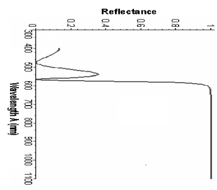
Figure 3: The spectral reflectance of a plant leaf according to the domain wall model, for $\lambda_{0}=400\,nm$ and $\delta=30\,nm$.

III. Results and discussions. The Figures 2 and 3 show the reflectance curves obtained experimentally via spectrum-radiometer LI-1800 from LI-COR and theoretically via domain wall model, respectively. As we can see in these figures, the model (Fig. 3) nicely simulates the real spectral behavior of a plant leaf (Fig. 2). In the visible region (400 a $700\,nm$) one observes two valley around $480\,nm$ and $680\,nm$ that evidences the absorption of the chlorophylls “b” and “a”, respectively, and a peak around $555\,nm$ that characterizes the color of a green plant leaf. In the near infrared region ($700\,nm$ - $1300\,nm$) the reflectance is almost constant. Let us now compare the results obtained experimentally with the results obtained theoretically via domain wall model, by entering with some known parameters of the model. We can use the formula below to estimate the critical wavelength

$$\lambda_{0}\!=\!\sqrt{\frac{A_{S}}{2\pi}}.$$ (19)

For structures (or spaces) with typical dimensions about 4-12 $\mu m$ of width and 10-14 $\mu m$ of length, as the regions separating spongy mesophylls, we find critical wavelength $\lambda_{0}\approx 400\,nm$. The parameter $\delta$ is associated with the domain wall thickness, and can be regarded as an effective thickness of the plant leaf, where effectively reflections may occur, i.e., the interior region of the plant leaf. The Fig. 3 shows the theoretical behavior of the spectral reflectance of a plant leaf according to our model. Unlike the spectral reflectance obtained experimentally (see Fig. 2) the minimal reflectance is zero because only internal effects are considered in the model. For the sake of simplicity, we disregard reflections from the surface of the plant leaf. Note that the spectral reflectance from internal structures of plant leaves is well approximated by our domain wall model. Although the second point of absorption around 565 $nm$ is a bit far from observed value 680 $nm$, the first point of absorption at 480 $nm$ is in perfect agreement and the reflectance peaked around 540 $nm$ is pretty close to the observed value around 555 $nm$ that characterizes the color of a green plant leaf.

IV. Conclusions. The model nicely simulates the spectral reflectance of a plant leaf as a function of the wavelength, i.e., its spectral behavior. The domain wall model works well for structures in the scale of micrometers ($\mu m$ ). This is also the scale of spaces between cells ( $\approx$ cellular walls thickness), that we can identify with the domain wall like structures in our model discussed above. In order to simulate better the spectral behavior of a plant leaf we expect to improve the model in a separate work. Such improvements may be concerned with the number and the type of domain walls like structures formed inside the domain wall that simulate the plant leaf. This may improve the description of several intercellular spaces giving the real complexity of the internal structure inside a plant leaf. Finally we should emphasize that our investigations concerning a domain wall model to simulate spectral reflectance here applied to a plant leaf can easily be extended to a class of planar systems with internal structures.

- (1) R.M. Hoffer, Biological and physical considerations in applying computer-aidded analysis techniques to remote sensor data, In. P.H. Swain, S.M. Davis, Eds. Remote Sensing the Quantitative Approach, (McGraw Hill, New York, 1978).
- (2) H.D.W. Gausman, Plant leaf optical properties in visible and near-infrared light, (Texas Tech, Lubbok, 1985).
- (3) D.M. Gates, Physical and physiological properties of plants. Remote sensing with special reference to agriculture and forestry, (National Academy of sciences, Washington D.C., 1970).
- (4) D.E. Bower, R.E. Davis, D.L. Myrick, K. Stocy, W.T. Jones, Spectral reflectances of natural targets for use in remote sensing studies, (Nasa reference publication 1139, Hampton, 1985).
- (5) A.R. Huet, Separation of soil-plant spectral mixtures by factor analysis, Remote Sen. Environ. 19, 237 (1986).
- (6) M.L.F. Freire, Spectral, agronomical, development and growth variations of a peanut crop caused by the phosphorous and calcium doses, (PhD Thesis -in Portuguese, Campina Grande - PB, Brazil, 2004).
- (7) T.M. Lillesan, R.W. Kiefer, Remote sensing and image interpretation, (John Willey and Sons, New York, 1987, 2nd Edition).
- (8) F.A. Brito, F. F. Cruz, J. F. N. Oliveira, Accelerating universes driven by bulk particles, Phys. Rev. D71, 083516 (2005).
- (9) F.A. Brito, D. Bazeia, Domain ribbons inside domain walls at finite temperature, Phys. Rev. D56, 7869 (1997).
- (10) D. Bazeia, R.F. Ribeiro, M.M. Santos, Topological defects inside domain walls, Phys. Rev. D54, 1852 (1996).
- (11) D. Bazeia, R.F. Ribeiro, M.M. Santos, Solitons in a class of systems of two coupled real scalar fields, Phys. Rev. E54, 2943 (1996).
- (12) D. Bazeia, J. R. S. Nascimento, R.F. Ribeiro, D. Toledo, Soliton stability in systems of two real scalar fields, J. Phys. A30, 8157 (1997).
- (13) J.R. Morris, Nested domain defects, Int. J. Mod. Phys. A13, 1115 (1998).
- (14) A. Vilenkin, E. P. S. Shellard, Cosmic strings and other topological defects (Cambridge UP, Cambridge/UK, 1994).