Aging and Immortality in a Cell Proliferation Model

Abstract

We investigate a model of cell division in which the length of telomeres within a cell regulates its proliferative potential. At each division, telomeres undergo a systematic length decrease as well as a superimposed fluctuation due to exchange of telomere DNA between the two daughter cells. A cell becomes senescent when one or more of its telomeres become shorter than a critical length. We map this telomere dynamics onto a biased branching diffusion process with an absorbing boundary condition whenever any telomere reaches the critical length. Using first-passage ideas, we find a phase transition between finite lifetime and immortality (infinite proliferation) of the cell population as a function of the influence of telomere shortening, fluctuations, and cell division.

I Introduction

Aging is a complex and incompletely understood process characterized by deteriorating cellular, organ, and system function. Replicative senescence, the phenomenon whereby normal somatic cells show a finite proliferative capacity, is thought to be a major contributor to this decline general . Telomeres are repetitive DNA sequences ((TTAGGG)_n in human cells) at both ends of each linear chromosome and their role is to protect the coding part of the DNA. Normal human somatic cells become senescent after a finite number of doublings.

As a general rule, cells for which telomerase activity is absent lose of the order of 100 base pairs of telomeric DNA from chromosome ends in every cell division. This basal loss has been attributed to the end replication problem Watson in which the DNA-polymerase cannot replicate all the way to the end of the chromosome during DNA lagging strand synthesis. Additional post-replicative processing of the telomeric DNA is necessary to protect the end of the chromosome from being recognized as a double strand break in need of repair. This processing also contributes to the end replication problem.

What remains unexplained, however, is why senescent cells occur in cell cultures long before the expected number of cell divisions estimated from the gradual basal loss. It has been shown recently that in addition to the basal loss of $\sim 100$ base pairs per division, a complex set of events that leads to telomere exchange between sister chromatids can occur. This telomere sister chromatid exchange (T-SCE), together with basal telomere loss and a number of observed or suggested telomere recombination events, collectively define telomere dynamics, and this dynamics leads to a wide distribution of telomere lengths in cell cultures TCE . Telomere exchange can also occur between the telomeres of different chromosomes. Currently available data cannot distinguish between this process and T-SCE. It is also believed that sister chromosome exchange is induced by DNA damage. Because the sister chromatids are in closer proximity compared to the distance between different chromatids, it can be hypothesize that the probability for telomere interchromatid exchange (T-ICE) is smaller than the probability for sister chromatid exchange between sister chromatids.

Recently, one of the present authors proposed a theory BlagoevGoodwin , based on telomere dynamics including T-SCE and T-ICE, that is capable of explaining Werner’s syndrome, an inherited disease characterized by premature aging and death, and a subset of cancers that seem to use a recombination mechanism to maintain telomere length. This latter mechanism, known as alternative lengthening of telomeres (ALT), as well as additional telomerase activity in some cases, are thought to contribute to the large proliferative potential of these cells ALT . Here proliferative potential denotes the time over which cells can continue to divide. In Ref. BlagoevGoodwin , we showed that both Werner’s syndrome and ALT can be described within the general framework of telomere dynamics in which there is an elevated rate of exchange of telomere DNA between two daughter cells, as observed in many experiments expt . One of the main numerical results from Ref. BlagoevGoodwin is a transition from finite to infinite proliferative potential in a cell culture as the parameters controlling the telomere recombination rates are varied.

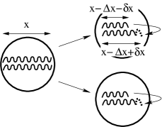
Figure 1: Schematic illustration of telomere evolution. The telomeres in the initial cell contain $x=15$ units. Upon division, each telomere ostensibly shortens by $\Delta x=5$ units, but additional exchange of $\delta x=\pm 2$ units between daughter telomeres (dashed) leads to final lengths of 8 and 12.

In this work, we analytically investigate an idealized model of cell proliferation in which the number of cell divisions before senescence occurs is controlled by the dynamics of telomeres during cell division. Each cell contains a certain number of telomeres. When a cell divides, the telomeres in each daughter cell ostensibly shorten by a fixed amount $\Delta x$. In addition to this systematic telomere shortening, the effect of T-SCE processes during cell division leads to a superimposed stochastic component to the telomere length dynamics by an amount $\delta x$ (Fig. 1). Thus in each cell division event, the length of an individual telomere evolves by the combined effects of these systematic and stochastic mechanisms.

When the length $x$ of any of the telomeres within a cell reaches zero, the cell stops dividing and becomes senescent. On the other hand, the stochastic component of the telomere dynamics provides the possibility for a telomere to occasionally grow when a cell divides. This sub-population of cells with long telomeres and thus higher proliferative potential can become even more so at the next cell division, a mechanism that allows a long-lived subpopulation to thrive.

We are interested in basic statistical properties of the cell proliferative potential. Some fundamental questions that we will study include:

1. Can a cell population divide indefinitely?

2. How long does it take for a cell population to become senescent?

3. How many dividing cells exist after a given number of divisions?

Within an idealized model of telomere kinetics described by Eq. (1) for a single telomere per cell, it is possible to answer these questions analytically by mapping the telomere dynamics to a first-passage process. Using this approach, we find a phase transition between a finite-lifetime cell population and immortality as a function of three basic control parameters—the magnitude of the systematic part of the telomere evolution, determined by $\Delta x$, the effective diffusion coefficient associated with the stochastic part of the telomere evolution, determined by $\langle\delta x(t)^{2}\rangle$, and the cell division rate.

II Telomere Replication Model

In our telomere replication model, we assume that the initial length of each telomere in a cell is $x_{0}$. In any cell division event, the length of a telomere changes by two distinct processes:

1. a systematic shortening of each telomere by $\Delta x$;

2. an additional stochastic component of the length change of magnitude $\delta x$.

Thus the length of a telomere changes according to

$$x\to x-\Delta x+\delta x.$$ (1)

Here the stochastic variable $\delta x$ accounts for the T-SCE processes that we assume to have mean value equal to zero, $\langle\delta x\rangle=0$, and no correlations at different times, $\langle\delta x(t)\delta x(t^{\prime})\rangle\propto\delta(t-t^{\prime})$. The justification for the absence of correlation is that T-SCE events have been linked to DNA damage TCE-justify , which occurs randomly in the cell.

Because of the systematic and stochastic contributions to the change in telomere length in each division event, the length of a telomere undergoes a biased random walk, with a bias toward shrinking. It is instructive to estimate the relative importance of the systematic and stochastic components of this length evolution. For this purpose, we define the time unit as the physical time between cell divisions $\delta t$. Thus in the absence of stochasticity a telomere shrinks to zero length in $x_{0}/\Delta x$ cell division events.

It is now helpful to recall some basic numbers about human telomeres to connect our mechanistic telomere model and real cell division:

parameter	definition	numerical value
$\delta t$	time between	20 minutes –
	cell divisions	several hours
$x_{0}$	initial telomere	$\approx 10^{4}$ base pairs
	length
$\Delta x$	systematic length	$\approx 10^{2}$ base pairs
	decrease per division
$\delta x$	stochastic length	$\approx 10^{2}$ base pairs
	decrease per division

The quantity $\delta x$ is known only very roughly. It is possible, with low probability, that even whole telomeres can be lost in TCE processes low-prob .

With the above numbers, a telomere shrinks to zero in $x_{0}/\Delta x\approx 10^{2}\equiv N$ cell division events with purely deterministic shrinking. Now consider the role of stochasticity: in $N$ cell divisions, the root-mean-square length change due to stochastic events is $\ell_{\rm rms}=\sqrt{N(\delta x)^{2}}\approx 10^{3}$. Thus in the time for a telomere to systematically shrink from $10^{4}$ to zero, stochasticity gives a length uncertainty of $10^{3}$—a 10% correction to the bias.

Finally, we need to include the role of cell division on this biased random walk description to arrive at a theory for telomere dynamics. That is, we need to allow a random walk to replicate as it undergoes biased hopping. While there are many ways to parameterize the effects of bias, stochasticity, and replication in the continuum limit, all such models lead to the following convection-diffusion equation with multiplicative growth:

$$\frac{\partial n(x,t)}{\partial t}=kn(x,t)+v\frac{\partial n(x,t)}{\partial x}+D\frac{\partial^{2}n(x,t)}{\partial x^{2}}\,,$$ (2)

in which $v$ represents the bias for telomere shrinking, $D$ accounts for the stochastic part of the telomere length evolution, and $k$ accounts for cell division. While there is only an indirect connection between the model parameters $v,D,k$, and the parameters $\Delta x,\delta x$ that account for what happens to a telomere in a single cell division, this continuum description has the advantage of capturing the physical essence of telomere dynamics while being analytically tractable.

The basic question that we seek to understand is how long it takes for a cell to become senescent, an event that occurs when the length of one of its telomeres reaches zero. This condition translates to an absorbing boundary condition at $x=0$ for the biased diffusion process that described the telomere length distribution. We now exploit some classic results about the first-passage probability of biased diffusion (see Appendix and fpp ) to determine the evolution of the telomere length distribution. Let the initial number of cells be $N_{0}$. The solution of (2) is simply

$$n(x,t)=N_{0}e^{kt}c(x,t)$$ (3)

where $c(x,t)$, given in (26), is the solution to the convection-diffusion equation with an absorbing boundary condition at $x=0$ and the initial condition that all cells have initial telomere length $x_{0}$.

We may also treat the situation in which each cell contains $M$ independent telomeres as a zeroth-order description for cells that contain many telomeres whose dynamics is coupled by the T-SCE exchange process (schematically illustrated in Fig. 1). This assumption of independence of different telomeres allows us to apply the single telomere per cell first-passage description with only minor modifications. For cells containing $M$ independent telomeres of lengths ${\mathbf{x}}=(x_{1},\dots,x_{M})$, the density of cells $n({\mathbf{x}},t)$ satisfies the $M$-dimensional convection-diffusion-growth equation

$$\frac{\partial n({\mathbf{x}},t)}{\partial t}=kn({\mathbf{x}},t)+v\nabla n({\mathbf{x}},t)+D\nabla^{2}n({\mathbf{x}},t)~{},$$ (4)

with absorbing boundaries when any telomere length $x_{i}$ reaches 0. The solution simply factorizes as a product of one-dimensional solutions

$$n({\mathbf{x}},t)=N_{0}e^{kt}\prod_{i=1}^{M}c(x_{i},t)~{}.$$ (5)

If each telomere has initial length $x_{0}$, all the $c(x_{i},t)$ are the same and are given by (26). We can also straightforwardly study the case where each telomere has a different initial length by merely using the unique initial length of each telomere in Eq. (5). It is worth mentioning that in addition to its application to cell division statistics, Eq. (4) is also related to the Fleming-Viot (FV) process FV in which a population of diffusing particles can get absorbed at boundary point and then be re-injected into the system at a rate that is proportional to local particle density.

From our description of telomere dynamics as a biased branching-diffusion process, we now determine basic features about the time dependence of the cell population and the statistics of telomere lengths.

II.1 Number of Dividing and Senescent Cells

Cells in which each telomere has positive length can divide. The number of such active cells is given by the integral of the number density of cells over the positive $2^{M}$-tant ($x_{1},x_{2},\ldots,x_{N}>0$) of length space:

$$N_{\rm active}(t)=\int_{{\mathbf{x}}>0}n({\bf x},t)\,d{\mathbf{x}}=N_{0}e^{kt}S^{M}(t)~{},$$ (6)

where $S(t)$ is the survival probability of a biased random walk (given by (28)). From (30), the long-time behavior of $N_{\rm active}(t)$ is given by

$$N_{\rm active}(t) \sim \Big{(}\sqrt{\frac{D}{\pi}}\frac{2x_{0}}{v^{2}}\Big{)}^{\!\!M}\!\!e^{Mvx_{0}/2D}~{}t^{-3M/2}~{}e^{(k-Mv^{2}/4D)t}\,,$$ (7)

$$\propto t^{-3M/2}~{}e^{kt(\epsilon_{M}-1)/\epsilon_{M}}\,,$$

with $\epsilon_{M}\equiv 4Dk/Mv^{2}$. Thus the fundamental parameters of the system are the Péclet number $P\!e\equiv vx_{0}/2D$ Pe , a dimensionless measure of the relative importance of the bias and the stochasticity and, more importantly, the dimensionless growth rate, $\epsilon_{M}$. Note that both the diffusion coefficient $D$ and the bias velocity $v$ are proportional to $k$, since the telomere length changes occur only when a cell divides. As a result, the growth rate $\epsilon_{M}$ is actually independent of $k$. For $\epsilon_{M}<1$, cell division is insufficient to overcome the effect of inexorable death due to the systematic component of the telomere shortening and the population of dividing cells decays exponentially in time.

Figure 2: Plot of the number of active cells versus time from the second line of Eq. (7) for the case of $M=1$ telomere per cell, with $\epsilon_{1}=0.8$ (solid) 0.9 (dashed), and 0.99 (dotted).

To get a feeling for the interplay between telomere shortening and cell division, let us employ the numerical parameters given at the beginning of this section in Eq. (7) to obtain the total number of dividing cells. Since cells double at each time step, $k=\ln 2$ when we express $t$ in units of cell division times. Furthermore, we define the coefficients $\alpha$ and $\beta$ by $v=\alpha\times 10^{2}$ and $D=\beta\times 10^{4}$. Then the time dependent exponential factor in (7) for the case $M=1$ becomes

$$e^{(k-v^{2}/4D)t}\sim e^{(\ln 2-\alpha^{2}/4\beta)t}\,.$$

The exponent can be either positive or negative exponent depending on $\alpha$ and $\beta$, which, in turn, depend on details of the telomere evolution a single cell division event. Thus, using the numbers appropriate for humans, senescence or immortality is controlled by details of telomere evolution as encoded by the coefficients $\alpha$ and $\beta$.

We also obtain the total number of cells that become senescent at any given time during the evolution as the diffusive flux to $x_{i}=0$ for any $i$. For the symmetric initial condition, the number of cells reaching any boundary $x_{i}=0$, $i=1,2,\ldots,M)$, are the same. Hence we may consider a single boundary, say $i=1$. The number of dying cells at this boundary can be written as the integral over the $x_{1}=0$ surface

$$J_{1}(t)=\int_{{{\mathbf{x}}>0}\atop x_{1}=0}D\,\frac{\partial n({\mathbf{x}},t)}{\partial x_{1}}\,d{\mathbf{x}}_{\perp}\,,$$ (8)

where the integral is over all the $M-1$ coordinates perpendicular to $x_{1}$. Note again the absence of a convective term in this expression because there is no convective flux when the concentration is zero. Using the product form (5) of $n({\mathbf{x}},t)$ for the total number of dying cells we obtain

$$J(t)=MJ_{1}(t)=N_{0}Me^{kt}F(t)S^{M-1}(t)$$ (9)

where $S(t)$ and $F(t)$ are given by (28) and (27) respectively. The total number of senescent cells that are produced during the course of the evolution is

$$N_{\rm sen} = \int_{0}^{\infty}J(t)\,dt=-N_{0}\int_{0}^{\infty}dt~{}e^{kt}~{}\frac{\partial S^{M}(t)}{\partial t}$$ (10)

$$= N_{0}\left[1-k\int_{0}^{\infty}dt~{}e^{kt}~{}S^{M}(t)\right]~{},$$

where we again use the fact that $F(t)=-dS(t)/dt$ to perform the integration by parts.

Figure 3: Plot of the total number of senescent cells that are produced during the evolution of the cell population as a function of the dimensionless growth rate $\epsilon_{1}=4Dk/v^{2}$.

For the special case of one telomere per cell ($M=1$) we have

$$J(t)=\frac{N_{0}x_{0}}{\sqrt{4\pi Dt^{3}}}\,\,e^{kt}\,\,e^{-(x_{0}-vt)^{2}/4Dt}.$$ (11)

In this case the total number of senescent cells is

$$N_{\rm sen}=\frac{N_{0}x_{0}}{\sqrt{4\pi D}}\,\int_{0}^{\infty}\frac{1}{t^{3/2}}\,\,e^{kt}\,\,e^{-(x_{0}-vt)^{2}/4Dt}dt.$$ (12)

We now make the substitution $z=t^{-1/2}$ to recast the above integral into the form

$$N_{\rm sen}=\frac{N_{0}x_{0}}{\sqrt{\pi D}}\,e^{vx_{0}/2D}\int_{0}^{\infty}dz\,\,e^{-x_{0}^{2}z^{2}/4D-(\frac{v^{2}}{4D}-k)/z^{2}}.$$ (13)

Using the $\int_{0}^{\infty}e^{-az^{2}-b/z^{2}}\,dz=\sqrt{\frac{\pi}{4a}}\,e^{-\sqrt{4ab}}$ from 3.325 of Ref. GR , we thus obtain

$$N_{\rm sen} = N_{0}e^{vx_{0}/2D}\,\exp\left[-\sqrt{\frac{v^{2}x_{0}^{2}}{4D}\Big{(}1-\frac{4Dk}{v^{2}}\Big{)}}\right]$$ (14)

$$= N_{0}e^{P\!e}\,\exp\left[-\sqrt{P\!e^{2}(1-\epsilon_{1})}\right],$$

which is plotted in Fig. 3 for the case $N_{0}=1$ and $P\!e=10$.

This result for $N_{\rm sen}$ holds only for $\epsilon_{1}<1$; this is the regime where the cell population eventually becomes senescent so that the total number of senescent cells produced during the evolution is finite. When $\epsilon_{1}\ll 1$, the leading behaviors of the two exponential factors in Eq. (14) cancel and $N_{\rm sen}\to(1+\epsilon_{1}/2P\!e)$. Thus as $\epsilon_{1}\to 0$ (no division), the initial cell immediately becomes senescent so that the total number of senescent cells that are produced equals one. This unrealistic result arises because in the continuum description telomeres can shrink to zero length before any cell division can occur. On the other hand, for $\epsilon_{1}>1$, the population is immortal and an infinite number of senescent cells are produced during the evolution.

II.2 Telomere Length Distribution

A curious aspect of the population of dividing cells is the dependence of the cell density on telomere length as $t\to\infty$. For any number of telomeres per cell $M$, the telomere length distribution is independent of this number, since the distribution is simply proportional to $c(x,t)$ in Eq. (26). In the $t\to\infty$ limit, we then obtain

$$c(x,t\to\infty) \propto \frac{xx_{0}}{\sqrt{4\pi(Dt)^{3}}}\,e^{-(v^{2}/4D)t-v(x-x_{0})/2D}$$ (15)

$$\propto xe^{-vx/2D}~{}.$$

Thus apart from an overall time-dependent factor, the density of dividing cells in which the constituent telomere has length $x$ is linear in $x$ for small lengths and has an exponential cutoff for large lengths. From the distribution given in Eq. (15), the mean telomere length goes to a constant for large times

$$\langle x\rangle=\frac{\int_{0}^{\infty}x\,c(x,t)\,dx}{\int_{0}^{\infty}c(x,t)\,dx}\to\frac{4D}{v}~{},$$ (16)

independent of whether the total cell population is growing or decaying. The variance of the telomere length also approaches a constant

$$\langle x^{2}\rangle-\langle x\rangle^{2}\to\frac{8D^{2}}{v^{2}}~{}.$$ (17)

A more pedantic way to arrive at this same result is to compute the exact time-dependent mean telomere length $\langle x(t)\rangle$ using Eq. (26) for $c(x,t)$ and then taking the $t\to\infty$ limit. In summary, the mean telomere length is time independent, as predicted by the asymptotic form of the telomere length distribution in Eq. (15). We emphasize that this result pertains to the fraction of cells that are active. If all cells—senescent and active—are included in the average, then $\langle x\rangle$ would asymptotically decay with time.

II.3 Mean Proliferative Potential and Immortality

As discussed above, for $\epsilon_{M}<1$, all cells eventually become senescent. However, for $\epsilon_{M}>1$, a subpopulation of infinitely dividing cells arise so that the average cell population becomes immortal. We make this statement more precise by computing the average lifetime of the population for $\epsilon_{M}<1$. This lifetime is defined as the average age of each cell when it becomes senescent and is thus given by

$$\langle t\rangle=\frac{\displaystyle\int_{0}^{\infty}t\,J(t)\,dt}{\displaystyle\int_{0}^{\infty}J(t)\,dt}=\frac{\displaystyle\int_{0}^{\infty}t\,e^{kt}F(t)S^{M-1}(t)\,dt}{\displaystyle\int_{0}^{\infty}e^{kt}F(t)S^{M-1}(t)\,dt}~{},$$ (18)

where we use (9) for $J(t)$, the number of cells that become senescent at time $t$. More simply, the mean proliferative potential (lifetime) can also be obtained from the total number of senescent cells via $\langle t\rangle=\frac{\partial}{\partial k}\ln N_{\rm sen}$.

Using the general definition of Eq. (18), it is straightforward to compute higher moments of the lifetime for the case $M=1$. Here the integrals in (18) can be written in terms of the modified Bessel functions of the second kind (see #12 in 3.471 of Ref. GR ) to give

$$\langle t^{\gamma}\rangle=\left(\frac{x_{0}^{2}}{v^{2}(1-\epsilon_{1})}\right)^{\gamma/2}\frac{K_{\gamma-1/2}(\sqrt{1-\epsilon_{1}}Pe/2)}{K_{-1/2}(\sqrt{1-\epsilon_{1}}Pe/2)}~{},$$ (19)

where $\gamma$ does not necessarily have to be an integer. Using this general formula the variance of the lifetime is

$$\langle t^{2}\rangle-\langle t\rangle^{2}=\frac{2Dx_{0}}{v^{3}(1-\epsilon_{1})^{3/2}}~{}.$$ (20)

In fact, the $n^{\rm th}$ cumulant can be obtained simply from the general formula K

$$C_{n}=\frac{\partial^{n}\ln N_{\rm sen}}{\partial k^{n}}.$$

Therefore for the higher moments of the lifetime, the diffusion coefficient does play an essential role.

For $M=1$, we immediately obtain from Eq. (14)

$$\langle t\rangle=\frac{x_{0}}{v}\,\frac{1}{\sqrt{1-\epsilon_{1}}}.$$ (21)

Thus the mean cell proliferative potential diverges to infinity as $\epsilon_{1}\to 1$ from below. This result for the number of cell divisions before senescence is one of our primary results. Notice that in the case of no cell division ($k=0$, $\epsilon_{1}=0$) the average lifetime $\langle t\rangle=x_{0}/v$. That is, $\langle t\rangle$ coincides with the time for a biased diffusing particle to be convected to the origin. It is surprising at first sight that diffusion plays no role in determining the average number of cell divisions. Exactly the same type of result arises for the discrete random walk with a bias $v$ kt .

II.4 Senescence Plateau

A useful characterization of the number of cell divisions distribution function of a population is the senescence rate $m(t)$. The senescence (or mortality) rate is the ratio of the number of cells that become senescent at time $t$ to the total number of cells that are still dividing at this time. Equivalently, the senescence rate is the probability that a randomly chosen dividing cell becomes senescent at the next moment. The senescence rate is thus given by

$$m(t)=\frac{J(t)}{N(t)}~{},$$ (22)

where the number of dying cells $J(t)$ and dividing cells $N(t)$ are given by Eqs. (9) and (6) respectively. Substituting these expressions into (22), we find that the senescence rate is independent of the number of telomeres per cell $M$, i.e.

$$m(t)=\frac{F(t)}{S(t)}=-\frac{\partial\ln S(t)}{\partial t}~{}.$$ (23)

Using the asymptotic form of $S(t)$ given in (30), the senescence rate approaches a time-independent value in the long-time limit and is given by

$$m(t)\simeq\frac{v^{2}}{4D}+\frac{3}{2t}+{\cal O}\left(\frac{1}{t^{2}}\right)~{}.$$ (24)

Amazingly, as the cell population ages, the senescence rate of the cells that remain dividing ultimately tends to a constant value for large times. This phenomenon is known as the mortality plateau. Namely, the probability that the somatic cells of an organism become senescent becomes independent of its age in the long-time limit. This surprising fact was observed experimentally in human populations humans and for fruit flies flies . It was also observed numerically in a model of aging that is similar to ours WF . The existence of such a senescence plateau is actually typical of a wide range of Markov processes evans .

III Summary

We studied an idealized model for the dynamics of telomere lengths during cell division that is based on a systematic basal loss and a stochastic component to the evolution that arises from telomere sister chromatid exchange. This model captures essential features of telomere dynamics in cell cultures. Because of the competing influences of cell division, which obviously increases the number of proliferative cells, and the general trend of telomere shortening, we showed that there is a phase transition between a normal state where a cell culture becomes senescent to a new state where a cell culture can become immortal.

From our theory, we were able to answer the basic questions posed in the introduction. Specifically:

1. We determined the condition for whether a cell population ultimately becomes senescent or whether it continues to divide ad infinitum. The transition between these two regimes is given by the condition $\epsilon_{M}=1$, where $\epsilon_{m}=4Dk/Mv^{2}$ is a dimensionless measure of the relative effect of cell division, random fluctuations, and basal loss in the length evolution of a telomere.

2. We also found that for the case of $M=1$ telomere per cell, the mean time for a cell population to become senescent is

   $$\langle t\rangle=\frac{x_{0}}{v}\frac{1}{\sqrt{1-\epsilon_{1}}}$$

   for $\epsilon_{1}<1$. Here $x_{0}$ is the initial length of the telomere, $v$ is the amount by which the telomere shrinks by basal loss in each division, and $\epsilon_{M}\equiv 4Dk/Mv^{2}$ is a dimension measure of the relative importance of cell division to basal loss.

3. Finally, we found that the total number of cells produced before the entire cell culture becomes senescent becomes extremely large as $\epsilon$ approaches its critical value from below, as presented in Eq. (14).

Our results may be helpful for understanding how ALT cells maintain their telomeres. In these cells, increased T-SCE rate, and wide telomere size distribution, and increased cell lifetimes have been observed TCE . These observations are all natural outcomes from our model. How these results depend on the number of short telomeres and on the details of the T-SCE process are very important questions that are under investigation.

Appendix A First-Passage for Biased Diffusion

We recall some basic results about first-passage for biased diffusion on the positive half line $x>0$ fpp that will be used to describe cell proliferation statistics. According to Eq. (1), the length of each telomere undergoes biased diffusion, in the continuum limit, with positive bias ($v>0$) defined to be directed towards smaller telomere length $x$. An absorbing boundary condition at the origin imposes the constraint that when $x$ reaches zero the cell effectively becomes senescent and is thus removed from the population of dividing cells.

Let $c(x,t)$ be the concentration of diffusing particles at $x$ at time $t$. The concentration evolves by the convection diffusion equation

$$\frac{\partial c(x,t)}{\partial t}=v\frac{\partial c(x,t)}{\partial x}+D\frac{\partial^{2}c(x,t)}{\partial x^{2}}\,,$$ (25)

For the initial condition $c(x,t=0)=\delta(x-x_{0})$, corresponding to a single particle starting at $x_{0}$, the concentration at any later time is fpp

$$\begin{split}c(x,t)=\frac{1}{\sqrt{4\pi Dt}}\,\Big{[}&e^{-(x-x_{0}+vt)^{2}/4Dt}\\ &-e^{+vx_{0}/D}\,e^{-(x+x_{0}+vt)^{2}/4Dt}\Big{]}.\end{split}$$ (26)

The second term represents the “image” contribution; notice that the bias velocity of the image is in the same direction as that of the initial particle. The exponential prefactor in the image term ensures that the absorbing boundary condition $c(x=0,t)=0$ is always fulfilled.

From this concentration profile, the first-passage probability, namely, the probability for a diffusing particle to hit the origin for the first time at time $t$, is

$$F(t)=D\frac{\partial c}{\partial x}-vc\,\,\Big{|}_{x=0}=\frac{x_{0}}{\sqrt{4\pi Dt^{3}}}\,\,e^{-(x_{0}-vt)^{2}/4Dt}.$$ (27)

The convective contribution to the flux, $-vc$, gives no contribution because $c=0$ at $x=0$. Until the particle hits the boundary it stays in the system; hence its survival probability is simply

$$\begin{split}S(t)\!=\!\int_{0}^{\infty}\!\!\!\!c(x,t)\,dx=\frac{1}{2}\Bigg{[}&{\rm erfc}\Big{(}\frac{vt-x_{0}}{\sqrt{4Dt}}\Big{)}\\ &-e^{vx_{0}/D}{\rm erfc}\Big{(}\frac{vt+x_{0}}{\sqrt{4Dt}}\Big{)}\Bigg{]},\end{split}$$ (28)

where ${\rm erfc}(z)$ is the complementary error function. Since there is only one absorbing point in the system, the survival probability and the first passage probability are related by

$$F(t)=-\frac{dS(t)}{dt}\,.$$ (29)

From the asymptotics of the error function AS , ${\rm erfc}(z)\sim e^{-z^{2}}/\sqrt{\pi}\,z$, the long-time behavior of $S(t)$ is given by

$$S(t) \sim \sqrt{\frac{Dt}{\pi}}\frac{2x_{0}}{(vt)^{2}-x_{0}^{2}}\,\,e^{kt}\,\,e^{-(vt-x_{0})^{2}/4Dt}$$ (30)

$$\sim \sqrt{\frac{D}{\pi}}\frac{2x_{0}}{v^{2}}~{}e^{vx_{0}/2D}~{}t^{-3/2}~{}e^{-(v^{2}/4D)t}.$$

As expected intuitively, the survival probability asymptotically decays exponentially with time because the bias drives the particle towards the absorbing point. This result is used in Eqs. (6) & (7) to determine the number of active cells as a function of time.

References

- (1) L. Hayflick, Exp. Cell Res. 37, 614 (1965); C. B. Harley, Mutation Res. 256, 271 (1991); J. Campisi, Cell 94, 497 (1996); Eur. J. Cancer 33 703 (1997); Trends Cell Biol. 11, S27 (2001).
- (2) J.D. Watson, Nat. New Biol. 239 197 (1972); A. M. Olovnikov, Dokl. Akad. Nauk SSSR, 201, 1496 (1971).
- (3) R. R. Reddel, Cancer Lett. 194, 155 (2003).
- (4) E. H. Goodwin and K. B. Blagoev, Proc. Second Cold Spring Harbor Laboratory Meeting on Molecular Genetics of Aging, (2004); K. B. Blagoev and E. H. Goodwin, Proc. Telomeres & Telomerase, Cold Spring Harbor Laboratory, (2005); K. B. Blagoev & E. H. Goodwin, submitted to Nature (2006).
- (5) T. M. Bryan, A. Englezou, L. Dalla-Pozza, M. A. Dunham, and R. R. Reddel, Nat. Med. 3, 1271 (1997); J. D. Henson, A. A. Neumann, T. R. Yeager, and R. R. Reddel, Oncogene 21, 598 (2002).
- (6) S. M. Bailey, M. A. Brenneman, and E. H. Goodwin, Nucleic Acids Res. 32 3743 (2004).
- (7) S. M. Bailey, M. N. Cornforth, A. Kurimasa, D. J. Chen and E. H. Goodwin, Science 293 2462 (2001).
- (8) S. Hasenmaile, G. Pawelec, and W. Wagner, Biogerontology, 4, 253 (2003).
- (9) S. Redner, A Guide to First-Passage Processes, (Cambridge University Press, New York, 2001).
- (10) W. H. Fleming and M. Viot, Indiana Univ. Math. J. 28 817 (1979); P. A. Ferrari and N. Marić, math.PR/0605665
- (11) For a general discussion on the meaning of the Péclet number, see e.g., R. F. Probstein, Physicochemical Hydrodynamics, 2nd ed. (John Wiley & Sons, 1994).
- (12) I. S. Gradshteyn and I. M. Ryzhik, Tables of Integrals, Series, and Products, (Academic Press, New York, 1965).
- (13) N. G. van Kampen Stochastic Processes in Physics and Chemistry, 2nd ed. (North-Holland, Amsterdam, 1997).
- (14) I. I. Gikhman and A. V. Skorokhod, Introduction to the Theory of Random Processes, (Dover, New York, 1969); S. Karlin and H. Taylor, A First Course in Stochastic Processes, (Academic Press, New York, 1975); R. M. Nisbet and W. S. C. Gurney, Modelling Fluctuating Populations, (John S. Wiley and Sons, New York, 1982).
- (15) J. W. Vaupel, in Between Zeus and the Salmon, The Biodemography of Longevity, chapter 2, pages 1737, K.W. Wachter and C.E. Finch, eds., (National Academies Press, Washington, D.C., 1997).
- (16) J. R. Carey, P. Liedo, D. Orozco, and J. W. Vaupel, Science, 258, 457, (1992).
- (17) J. S. Weitz and H. B. Fraser, Proc. Natl. Acad. Sci. USA 98, 15383 (2001). In their notation the plateau value, namely, the asymptotic hazard rate, is .
- (18) D. Steinsaltz and S. N. Evans, q-bio.PE/0608008 (to appear in Trans. Amer. Math. Soc.).
- (19) M. Abramowitz and I. A. Stegun, Handbook of Mathematical Functions (Dover Publications Inc., New York, 1970).