Calculating event-triggered average synaptic conductances
from the membrane potential

Abstract

The optimal patterns of synaptic conductances for spike generation in central neurons is a subject of considerable interest. Ideally, such conductance time courses should be extracted from membrane potential (V_m) activity, but this is difficult because the nonlinear contribution of conductances to the V_m renders their estimation from the membrane equation extremely sensitive. We outline here a solution to this problem based on a discretization of the time axis. This procedure can extract the time course of excitatory and inhibitory conductances solely from the analysis of V_m activity. We test this method by calculating spike-triggered averages of synaptic conductances using numerical simulations of the integrate-and-fire model subject to colored conductance noise. The procedure was also tested successfully in biological cortical neurons using conductance noise injected with dynamic-clamp. This method should allow the extraction of synaptic conductances from V_m recordings in vivo.

Introduction

Determining the optimal features of stimuli which are needed to obtain a given response is of considerable interest, for example in sensory physiology. Reverse-correlation is one of the most-used methods to obtain such estimates (Agüera y Arcas and Fairhall, 2003; Badel et al., 2006) and, in particular, the spike-triggered average (STA) is often used to determine optimal features linked to the genesis of action potentials (de Boer and Kuypers, 1968). The STA can be used to explore which feature of stimulus space the neuron is sensitive to, or to identify modes that contribute either to spiking or to the period of silence before the spike (Agüera y Arcas and Fairhall, 2003). Using intracellular recordings, it is straightforward to calculate the STA of the membrane potential (V_m), which yields the mean voltage trajectory preceding spikes. In contrast, it is much harder to determine the underlying synaptic conductance. Straightforward methods like recording at several different DC levels and estimating the total conductance from the ratio $\Delta I/\Delta V$ fail, since the presence of a voltage threshold necessitates $\Delta V\rightarrow 0$ at the time of the spike, which, in turn, artificially suggests a divergence of the total conductance to infinity. Similarly, solving the membrane equation for excitatory and inhibitory conductances separately suffers from an additional complication: because the distance to threshold changes, the time courses of the average synaptic conductances depend on the injected current.

Recent contributions (Badel et al., 2006; Paninski 2006a, 2006b) gave analytical expressions for the most likely voltage path, which in the low-noise limit approximates the STA, of the leaky integrate-and-fire (IF) neuron. In those cases, gaussian white noise current was considered as input. In Badel et al. (2006), a second state variable was added in order to obtain biophysically more realistic behavior. In Paninski (2006a, 2006b), in addition the exact voltage STA for the non-leaky IF neuron was computed, as well as the STA input current in discrete time. Here, a strong dependence of the STA shape on the time resolution $dt$ was found without a stable limit as $dt\rightarrow 0$. It was argued heuristically that this behavior results from the fact that decreasing the time step corresponds to increasing the bandwidth of the input current, a point which was supported by numerical simulations (Paninski et al., 2004; Pillow and Simoncelli, 2003), in which a pre-filtering of the white noise input results in a stable limit STA.

In this article, we focus on the problem of estimating the optimal conductance patterns required for spike initiation, based solely on the analysis of V_m activity. We consider neurons subject to conductance-based synaptic noise at both excitatory and inhibitory synapses. By discretizing the time axis, it is possible to obtain the probability distribution of conductance time courses that are compatible with the observed voltage STA. Due to the symmetry properties of the probability distribution, the STA time course of excitatory and inhibitory conductances can then be extracted by choosing the one with maximum likelihood. We test this method in numerical simulations of the IF model, as well as in real cortical neurons using the dynamic-clamp technique, by comparing the estimated STA with the real STA deduced from the injected conductances.

Material and Methods

Models

We considered neurons driven by synaptic noise described by two independent sources of colored conductance noise (point-conductance model (Destexhe et al., 2001)). The membrane equation of this system is given by:

$$C\frac{dV(t)}{dt} = -g_{L}\big{(}V(t)-V_{L}\big{)}-g_{e}(t)\big{(}V(t)-V_{e}\big{)}-g_{i}(t)\big{(}V(t)-V_{i}\big{)}+I_{DC},$$ (1)

$$\frac{dg_{s}(t)}{dt} = -\frac{1}{\tau_{s}}\big{(}g_{s}(t)-g_{s0}\big{)}+\sqrt{\frac{2\sigma_{s}^{2}}{\tau_{s}}}\xi_{s}(t),$$ (2)

Here, $g_{L}$, $g_{e}(t)$ and $g_{i}(t)$ are the conductances of leak, excitatory and inhibitory currents, $V_{L}$, $V_{e}$, $V_{i}$ are their respective reversal potentials, $C$ is the capacitance and $I_{DC}$ a constant current. The subscript $s$ in Eq. (2) can take the values $e,i$, which in turn indicate the respective excitatory or inhibitory channel. We use $g_{s0}$ and $\sigma_{s}$ to indicate the mean and standard deviation (SD) of the conductance distributions, $\xi_{s}(t)$ are gaussian white noise processes with zero mean and unit standard deviation. Throughout this article we use the correlation times $\tau_{e}=2.728$ ms and $\tau_{i}=10.49$ ms.

This system was solved using numerical simulations of the leaky IF model, which was adjusted to match recordings of cortical neurons in slices (threshold $-55$ mV, refractory period $3$ ms, reset $-75$ mV). Simulations were done using the NEURON simulation environment (Hines and Carnevale, 1997). To calculate STAs, approximately 1000 spikes occurring during spontaneous activity were used, each being preceded by a period of at least $100$ ms of silence to avoid “contamination” of the V_m STA by preceding spikes. The same analysis protocols (see Results) were applied to the model and to experimental data.

In order to address the influence of a dendritic filter on the reliability of our method, we used a two-compartment model based on that by Pinsky and Rinzel (1994). We removed all active channels and replaced them by an integrate-and-fire mechanism at the soma. The geometry (L = 3.18 $\mu$m, diam = 10 $\mu$m) as well as the parameters not related to the spiking mechanism ($g_{L}=10^{-4}$ S/cm², $V_{L}=-60$ mV, capacitance $c_{m}=3~{}\mu$F/cm², axial resistance $R_{a}=5.87\times 10^{5}~{}\Omega$cm) are identical for the two compartments. In addition, we chose a threshold for spiking V${}_{t}=-55$ mV at the soma. The parameters for leak conductance and capacitance needed for the estimation of the STAs of synaptic conductances from the V_m, $g^{so}_{L}$ and $C^{so}$, were obtained by current pulse injection into the soma at the resting state. The superscript $so$ indicates that these are effective values at the level of the soma. The values used were $g^{so}_{L}$ = 0.198 nS and $C^{so}$ = 5.86 pF. The parameters describing the distributions of synaptic conductances were chosen in a way such that the mean inhibitory conductance was four times that of excitation, and the latter was comparable to the leak conductance ($g_{e0}$ = 0.15 nS, $g_{i0}$ = 0.6 nS). Standard deviations were assumed to be one third of the respective means ($\sigma_{e}$ = 0.05 nS, $\sigma_{i}$ = 0.2 nS).

In vitro experiments

In vitro experiments were performed on 0.4 mm thick coronal or sagittal slices from the lateral portions of guinea-pig occipital cortex. Guinea-pigs, 4-12 weeks old (CPA, Olivet, France), were anesthetized with sodium pentobarbital (30 mg/kg). The slices were maintained in an interface style recording chamber at 33-35${\,}^{\circ}C$. Slices were prepared on a DSK microslicer (Ted Pella Inc., Redding, CA) in a slice solution in which the NaCl was replaced with sucrose while maintaining an osmolarity of 307 mOsm. During recording, the slices were incubated in slice solution containing (in mM): NaCl, 124; KCl, 2.5; MgSO₄, 1.2; NaHPO₄, 1.25; CaCl₂, 2; NaHCO₃, 26; dextrose, 10, and aerated with 95% O₂, 5% CO₂ to a final pH of 7.4. Intracellular recordings following two hours of recovery were performed in deep layers (layer IV, V and VI) in electrophysiologically identified regular spiking and intrinsically bursting cells. Electrodes for intracellular recordings were made on a Sutter Instruments P-87 micropipette puller from medium-walled glass (WPI, 1BF100) and beveled on a Sutter Instruments beveler (BV-10M). Micropipettes were filled with 1.2 to 2 M potassium acetate and had resistances of 80-100 M$\Omega$ after beveling.

The dynamic-clamp technique (Robinson et al., 1993; Sharp et al., 1993) was used to inject computer-generated conductances in real neurons. Dynamic-clamp experiments were run using the hybrid RT-NEURON environment (developed by G. Le Masson, Université de Bordeaux), which is a modified version of NEURON (Hines and Carnevale, 1997) running under the Windows 2000 operating system (Microsoft Corp.). NEURON was augmented with the capacity of simulating neuronal models in real time, synchronized with the intracellular recording. To achieve real-time simulations as well as data transfer to the PC for further analysis, we used a PCI DSP board (Innovative Integration, Simi Valley, USA) with 4 analog/digital (inputs) and 4 digital/analog (outputs) 16 bits converters. The DSP board constrains calculations of the models and data transfers to be made with a high priority level by the PC processor. The DSP board allows input (for instance the membrane potential of the real cell incorporated in the equations of the models) and output signals (the synaptic current to be injected into the cell) to be processed at regular intervals (time resolution = 0.1 ms). A custom interface was used to connect the digital and analog inputs/outputs signals of the DSP board with the intracellular amplifier (Axoclamp 2B, Axon Instruments) and the data acquisition systems (PC-based acquisition software ELPHY, developed by G. Sadoc, CNRS Gif-sur-Yvette, ANVAR and Biologic). The dynamic-clamp protocol was used to insert the fluctuating conductances underlying synaptic noise in cortical neurons using the point-conductance model, similar to a previous study (Destexhe et al., 2001). According to Eq. (1) above, the injected current is determined from the fluctuating conductances $g_{e}(t)$ and $g_{i}(t)$ as well as from the difference of the membrane voltage from the respective reversal potentials, $I_{DynClamp}=-g_{e}\big{(}V-V_{e}\big{)}-g_{i}\big{(}V-V_{i}\big{)}$.

All research procedures concerning the experimental animals and their care adhered to the American Physiological Society’s Guiding Principles in the Care and Use of Animals, to the European Council Directive 86/609/EEC and to European Treaties series no. 123, and was also approved by the local ethics committee “Ile-de-France Sud” (certificate no. 05-003).

Results

We first explain the method for extracting STAs from V_m activity, then we present tests of this method using numerical simulations and intracellular recordings in dynamic-clamp.

Method to extract conductance STA

The procedure we follow here to estimate STA of conductances from V_m activity is based on a discretization of the time axis. With this approach, a probability distribution can be constructed whose maximum gives the most likely conductance path compatible with the STA of the V_m. This maximum is determined by a system of linear equations which is solvable if the means and variances of conductances are known (for a method to estimate conductance mean and variance, see Rudolph et al., 2004).

We start from the voltage STA, which is an average over an ensemble of event-triggered voltage traces. Its relation to the conductance STAs is determined by the ensemble average of Eqs. (1) and (2). In general, there is a strong correlation (or anti-correlation) between $V(t)$ and $g_{s}(t)$ in time. However, it is safe to assume that there is no such correlation across the ensemble, since the noise processes $\xi_{s}(t)$ corresponding to each realization are uncorrelated. Also, the ensemble average is commutative with the time derivative. Thus, we can rewrite Eqs. (1) and (2) to obtain

$$\frac{d\langle V(t)\rangle_{x}}{dt} = -\frac{1}{\tau_{L}}\big{(}\langle V(t)\rangle_{x}-V_{L}\big{)}$$

$$-\frac{\langle g_{e}(t)\rangle_{x}}{C}\big{(}\langle V(t)\rangle_{x}-V_{e}\big{)}-\frac{\langle g_{i}(t)\rangle_{x}}{C}\big{(}\langle V(t)\rangle_{x}-V_{i}\big{)}+\frac{I_{DC}}{C},$$

$$\frac{d\langle g_{s}(t)\rangle_{x}}{dt} = -\frac{1}{\tau_{s}}\big{(}\langle g_{s}(t)\rangle_{x}-g_{s0}\big{)}+\sqrt{\frac{2\sigma_{s}^{2}}{\tau_{s}}}\langle\xi_{s}(t)\rangle_{x},$$ (4)

where $\tau_{L}=C/g_{L}$ and $\langle.\rangle_{x}$ denotes the ensemble average. In other words, the time evolution Eqs (1) and (2) also hold in terms of ensemble averages. In the following, we drop the bracket notation for legibility, but assume we are dealing with ensemble averaged quantities unless otherwise stated.

We discretize Eq. (Method to extract conductance STA) in time with a step-size $\Delta t$ and solve for $g_{i}^{k}$,

$$g_{i}^{k}=-\frac{C}{V^{k}-V_{i}}\left\{\frac{V^{k}-V_{L}}{\tau_{L}}+\frac{g_{e}^{k}(V^{k}-V_{e})}{C}+\frac{V^{k+1}-V^{k}}{\Delta t}-\frac{I_{DC}}{C}\right\}.$$ (5)

Since the series $V^{k}$ for the voltage STA is known, $g_{i}^{k}$ has become a function of $g_{e}^{k}$. In the same way, we solve Eq. (4) for $\xi_{s}^{k}$, which have become gaussian distributed random numbers,

$$\xi_{s}^{k}=\frac{1}{\sigma_{s}}\sqrt{\frac{\tau_{s}}{2\Delta t}}\left(g_{s}^{k+1}-g_{s}^{k}\Big{(}1-\frac{\Delta t}{\tau_{s}}\Big{)}-\frac{\Delta t}{\tau_{s}}g_{s0}\right).$$ (6)

There is a continuum of combinations $\{g_{e}^{k+1},g_{i}^{k+1}\}$ that can advance the membrane potential from $V^{k+1}$ to $V^{k+2}$, each pair occurring with a probability

$$p^{k} := p(g_{e}^{k+1},g_{i}^{k+1}|g_{e}^{k},g_{i}^{k})=\frac{1}{2\pi}e^{-\frac{1}{2}(\xi_{e}^{k2}+\xi_{i}^{k2})}=\frac{1}{2\pi}e^{-\frac{1}{4\Delta t}X^{k}},$$ (7)

$$X^{k} = \frac{\tau_{e}}{\sigma_{e}^{2}}\left(g_{e}^{k+1}-g_{e}^{k}\Big{(}1-\frac{\Delta t}{\tau_{e}}\Big{)}-\frac{\Delta t}{\tau_{e}}g_{e0}\right)^{2}$$

$$+\frac{\tau_{i}}{\sigma_{i}^{2}}\left(g_{i}^{k+1}-g_{i}^{k}\Big{(}1-\frac{\Delta t}{\tau_{i}}\Big{)}-\frac{\Delta t}{\tau_{i}}g_{i0}\right)^{2},$$

where we have used Eq. (6). Note that because of Eq. (5), $g_{e}^{k}$ and $g_{i}^{k}$ are not independent and $p^{k}$ is, thus, a unidimensional distribution only. Given initial conductances $g_{s}^{0}$, we can now write down the probability $p$ for certain series of conductances $\{g_{s}^{j}\}_{j=0,\ldots,n}$ to occur that reproduce a given voltage trace $\{V^{l}\}_{l=1,\ldots,n+1}$:

$$p=\prod_{k=0}^{n-1}p^{k}.$$ (9)

Due to the symmetry of the distribution $p$, the average paths of the conductances coincide with the most likely ones, so the cumbersome task of solving nested gaussian integrals can be circumvented. Instead, in order to determine the conductance series with extremal likelihood, we solve the n-dimensional system of linear equations

$$\left\{\frac{\partial X}{\partial g_{e}^{k}}=0\right\}_{k=1,\ldots,n},$$ (10)

where $X=\sum_{k=0}^{n-1}X^{k}$, for the vector $\{g_{e}^{k}\}$. This is equivalent to solving $\{\frac{\partial p}{\partial g_{e}^{k}}=0\}_{k=1,\ldots,n}$ and involves the numerical inversion of an $n\times n$-matrix. Since the system of equations is linear, if there is a solution for $\{g_{e}^{k}\}$, plausibility arguments suggest that it is the most likely (rather than the least likely) excitatory conductance time course. The series $\{g_{i}^{k}\}$ is then obtained from Eq. (5).

Test of the accuracy of the method using numerical simulations

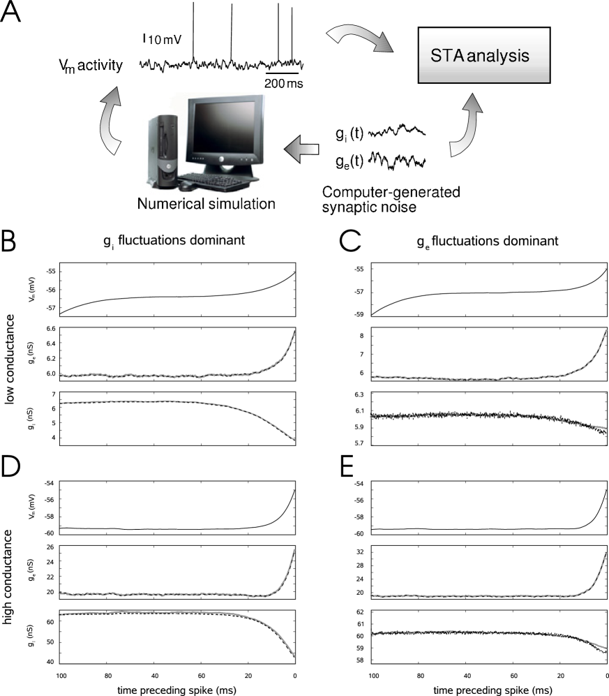
Figure 1: Test of the STA analysis method using an IF neuron model subject to colored conductance noise. A. Scheme of the procedure used. An IF model with synaptic noise was simulated numerically (bottom) and the procedure to estimate STA was applied to the V_m activity (top). The estimated conductance STAs from V_m were then compared to the actual conductance STA in this model. Bottom panels: STA analysis for different conditions, low-conductance states (B,C), high-conductance states (D,E), with fluctuations dominated by inhibition (B,D) or by excitation (C,E). For each panel, the upper graph shows the voltage STA, the middle graph the STA of excitatory conductance, and the lower graph the STA of inhibitory conductance. Solid lines (grey) show the average conductance recorded from the simulation, while the dashed line (black) represents the conductance estimated from the V_m. Parameters in B: $g_{e0}$=6 nS, $g_{i0}$=6 nS, $\sigma_{e}$=0.5 nS, $\sigma_{i}$=1.5 nS; C: $g_{e0}$=6 nS, $g_{i0}$=6 nS, $\sigma_{e}$=1.5 nS, $\sigma_{i}$=0.5 nS; D: $g_{e0}$=20 nS, $g_{i0}$=60 nS, $\sigma_{e}$=4 nS, $\sigma_{i}$=12 nS; E: $g_{e0}$=20 nS, $g_{i0}$=60 nS, $\sigma_{e}$=6 nS, $\sigma_{i}$=3 nS

To test this method, we first considered numerical simulations of the IF model in four different situations. We distinguished high-conductance states, where the total conductance is dominated by inhibition, from low-conductance states, where both synaptic conductances are of comparable magnitude. We also varied the standard deviations of the conductances such that for both high- and low-conductance states we have the cases $\sigma_{i}>\sigma_{e}$ as well as $\sigma_{e}>\sigma_{i}$. The results are summarized in Fig. 1, where the STA traces of excitatory and inhibitory conductances recorded from simulations are compared to the most likely (equivalent to the average) conductance traces obtained from solving Eq. (10). In general, the plots demonstrate a very good agreement.

To quantify our results, we investigated the effect of the statistics as well as of the broadness of the conductance distributions on the quality of the estimation. The latter is crucial, because the derivation of the most likely conductance time course allows for negative conductances, whereas in the simulations negative conductances lead to numerical instabilities, and conductances are bound to positive values. We thus expect an increasing error with increasing ratio SD/mean of the conductance distributions. We estimated the root-mean-square (RMS) of the difference between the recorded and the estimated conductance STAs. The results, summarized in Fig. 2, are as expected. Increasing the number of spikes enhances the match between theory and simulation (Fig. 2A shows the RMS deviation for excitation, 2B for inhibition) up to the point where the effect of negative conductances becomes dominant. In this example, where the ratio SD/mean was fixed at $0.1$, the RMS deviation enters a plateau at about $7000$ spikes. The plateau values can also be recovered from the neighboring plots (i.e., the RMS deviations at SD/mean $=0.1$ in Fig. 2C and D correspond to the plateau values in A and B). On the other hand, a broadening of the conductance distribution yields a higher deviation between simulation and estimation. However, at SD/mean $=0.5$, the RMS deviation is still as low as $\sim 2\%$ of the mean conductance for excitation and $\sim 4\%$ for inhibition.

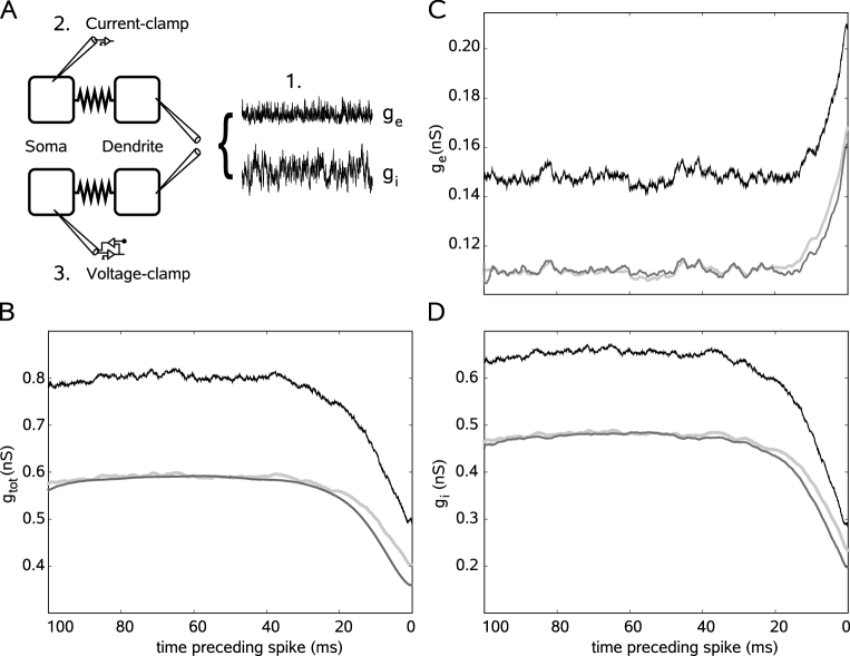
Figure 3: Test of the method using dendritic conductances. A. Simulation scheme: A 100 s sample of excitatory and inhibitory (frozen) conductance noise was injected into the dendrite of a 2-compartment model (1). Then, two different recording protocols were performed at the soma. First, the V_m time course was recorded in current-clamp (2), second, the currents corresponding to two different holding potentials were recorded in voltage-clamp (3). From the latter, the excitatory and inhibitory conductance time courses were extracted using Eq. 11. B. STA of total conductance inserted at the dendrite (black), compared with the estimate obtained in voltage-clamp (light gray) and with that obtained from somatic V_m activity using the method (dark gray). Due to dendritic attenuation, the total conductance values measured are lower than the inserted ones, but the variations of conductances preceding the spike are conserved. C. Same as B, for excitatory conductance. D. Same as B, for inhibitory conductance. Parameters: $g_{e0}=0.15$ nS, $g_{i0}=0.6$ nS, $\sigma_{e}=0.05$ nS, $\sigma_{i}=0.2$ nS, $g^{so}_{e0}=0.113$ nS, $g^{so}_{i0}=0.45$ nS, $\sigma^{so}_{e}=0.034$ nS, $\sigma^{so}_{i}=0.12$ nS, where the superscript $so$ denotes quantities as seen at the soma.

To assess the effect of dendritic filtering on the reliability of the method, we used a two-compartment model based on that of Pinsky and Rinzel (1994), from which we removed all active channels and replaced them by an integrate-and-fire mechanism at the soma. We repeatedly injected the same 100 s sample of fluctuating excitatory and inhibitory conductances in the dendritic compartment and performed two different recording protocols at the soma (Fig. 3A). First, we recorded in current-clamp in order to obtain the V_m time course as well as the spike times. In this case, the leak conductance $g^{so}_{L}$ and the capacitance $C^{so}$ were obtained from current pulse injection at rest. Second, we simulated an “ideal” voltage-clamp (no series resistance) at the soma using two different holding potentials (we chose the reversal potentials of excitation and inhibition, respectively). Then, from the currents $I_{V_{e}}$ and $I_{V_{i}}$, one can calculate the conductance time courses as

$$g^{so}_{e,i}(t)=\frac{I_{V_{i,e}}(t)-g_{L}(V_{i,e}-V_{L})}{V_{i,e}-V_{e,i}},$$ (11)

where the superscript $so$ indicates that these are the conductances seen at the soma (in the following referred to as somatic conductances). From these, we determined the parameters $g^{so}_{e0}$, $g^{so}_{i0}$, $\sigma^{so}_{e}$ and $\sigma^{so}_{i}$, the conductance means and standard deviations. In contrast to $g_{e}(t)$ and $g_{i}(t)$, the distributions of $g^{so}_{e}(t)$ and $g^{so}_{i}(t)$ are not Gaussian (not shown), and have lower means and variances. We compared the STA of the injected (dendritic) conductance, the STA obtained from the somatic V_m using our method and the STA obtained using a somatic “ideal” voltage-clamp (see Fig. 3B-D), which demonstrated the following points: (1) as expected, due to dendritic attenuation, all somatic estimates were attenuated compared to the actual conductances injected in dendrites (compare light and dark gray curves, soma, with black curve, dendrite, in Fig. 3B-D); (2) the estimate obtained by applying the present method to the somatic V_m (dark gray curves in Fig. 3B-D) was very similar to that obtained using an “ideal” voltage-clamp at the soma (light gray curves). The difference close to the spike may be due to the non-Gaussian shape of the somatic conductance distributions, whose tails then become important; (3) despite attenuation, the qualitative shape of the conductance STA was preserved. We conclude that the STA estimate from V_m activity captures rather well the conductances as seen by the spiking mechanism.

Test of the method in real neurons

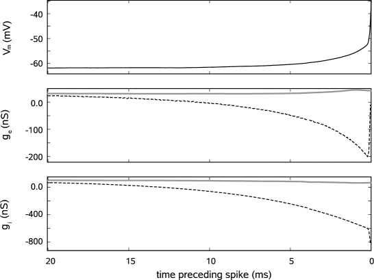
Figure 4: The effect of the presence of additional voltage-dependent conductances on the estimation of the synaptic conductances. Gray, solid lines indicate recorded conductances; black, dotted lines indicate estimated conductances. In this case, the estimation fails. The sharp rise of the voltage in the last ms before the spike requires very fast changes in the synaptic conductances, which introduces a considerable error in the analysis. Parameters used: $g_{e0}$=32 nS, $g_{i0}$=96 nS, $\sigma_{e}$=8 nS, $\sigma_{i}$=24 nS.

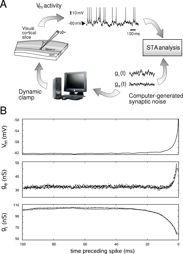
Figure 5: Test of the method in real neurons using dynamic-clamp in guinea-pig visual cortical slices. A. Scheme of the procedure. Computer-generated synaptic noise was injected in the recorded neuron under dynamic-clamp (bottom). The V_m activity obtained (top) was then used to extract the STA of conductances, which was compared to the STA directly obtained from the injected conductances. B. Results of this analysis in a representative neuron. Black lines show the estimated STA of conductances from V_m activity, grey lines show the STA of conductances that were actually injected into the neuron. The analysis was made by excluding the data from the 1.2 ms before the spike to avoid contamination by voltage-dependent conductances. Parameters for conductance noise were as in Fig. 4.

We also tested the method on voltage STAs obtained from dynamic-clamp recordings of guinea-pig cortical neurons in slices. In real neurons, a problem is the strong influence of spike-related voltage-dependent (presumably sodium) conductances on the voltage time course. Since we maximize the global probability of $g_{e}(t)$ and $g_{i}(t)$, the voltage in the vicinity of the spike has an influence on the estimated conductances at all times. As a consequence, without removing the effect of sodium, the estimation fails (see Fig. 4). Fortunately, it is rather simple to correct for this effect by excluding the last 1–2 ms before the spike from the analysis. The corrected comparison between the recorded and the estimated conductance traces is shown in Fig. 5.

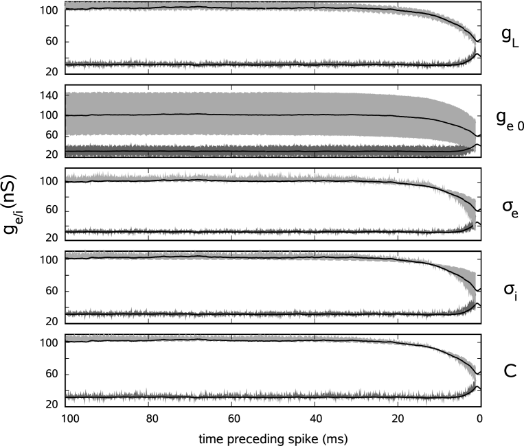
Figure 6: Deviation in the estimated conductance STAs in real neurons using dynamic-clamp due to variations in the parameters. The black lines represent the conductance STA estimates using the correct parameters, the gray areas are bound by the estimates that result from variation of a single parameter (indicated on the right) by $\pm$ 50 %. Light gray areas represent inhibition, dark gray areas represent excitation. The total conductance (leak plus synaptic conductances) was assumed to be fixed. A variation in the mean values of the conductances evokes mostly a shift in the estimate, while a variation in the SDs influences the curvature just before the spike.

Finally, to check for the applicability of this method to in vivo recordings, we assessed the sensitivity of the estimates with respect to the different parameters by varying the values describing passive properties and synaptic activity. We assume that the total conductance can be constrained by input resistance measurements, and that time constants of the synaptic currents can be estimated by power spectral analyses (Destexhe and Rudolph, 2004). This leaves $g_{L}$, $C$, $g_{e0}$, $\sigma_{e}$ and $\sigma_{i}$ as the main parameters. The impact of these parameters on STA conductance estimates is shown in Fig. 6. Varying these parameters within $\pm 50\%$ of their nominal value led to various degrees of error in the STA estimates. The dominant effect of a variation in the mean conductances is a shift in the estimated STAs, whereas a variation in the SDs changes the curvature just before the spike.

To address this point further, we fitted the estimated conductance STAs with an exponential function:

$$f_{s}(t)=G_{s}(1+K_{s}e^{\frac{t-t_{0}}{T_{s}}}),$$

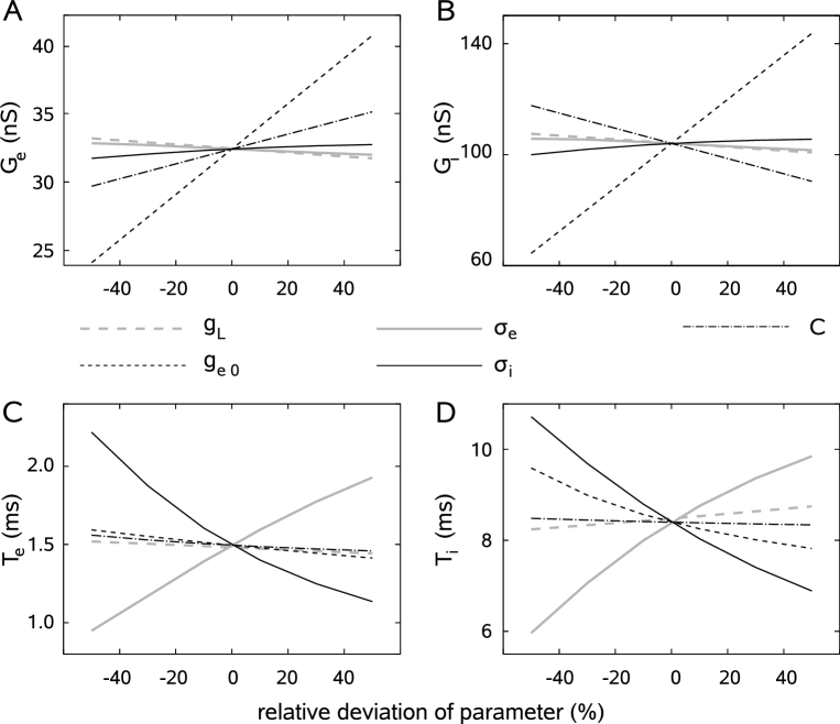
Figure 7: Detailed evaluation of the sensitivity to parameters. The conductance STAs were fitted with an exponential function $f_{s}(t)=G_{s}(1+K_{s}exp((t-t_{0})/T_{s})$, $s=e,i$. $t_{0}$ is chosen to be the time at which the analysis stops. Each plot shows the estimated value of $G_{e}$, $G_{i}$, $T_{e}$ or $T_{i}$ from this experiment, each curve represents the variation of a single parameter (see legend).

where $s$ again takes the values $e,i$ for excitation and inhibition, respectively. $t_{0}$ is chosen to be the time at which the analysis stops. Fig. 7 gives an overview of the dependence of the fitting parameters $G_{e}$, $G_{i}$, $T_{e}$ and $T_{i}$ on the relative change of $g_{L}$, $g_{e0}$, $\sigma_{e}$, $\sigma_{i}$ and $C$. For example, a variation of $g_{e0}$ has a strong effect on $G_{e}$ and $G_{i}$, but affects to a lesser extent $T_{e}$ and $T_{i}$, while the opposite was seen when varying $\sigma_{e}$ and $\sigma_{i}$.

Discussion

Understanding the transfer function of a neuron from synaptic input to spike output would ideally require the simultaneous monitoring of both the synaptic conductances and the cell’s firing. Current methods for extracting synaptic conductances rely on intracellular recordings performed at different holding potentials (in voltage-clamp) or different current levels (in current-clamp; e.g. Borg-Graham et al. 1998) and, as a consequence, they do not allow the establishment of a direct correspondence between synaptic conductances and spikes. Although these methods have been very useful, for example in establishing the synaptic structure of sensory receptive fields in a variety of systems (Monier et al., 2003; Wehr and Zador, 2003; Wilent and Contreras, 2005), they do not distinguish between trials that effectively produce spikes at a given latency and those that do not.

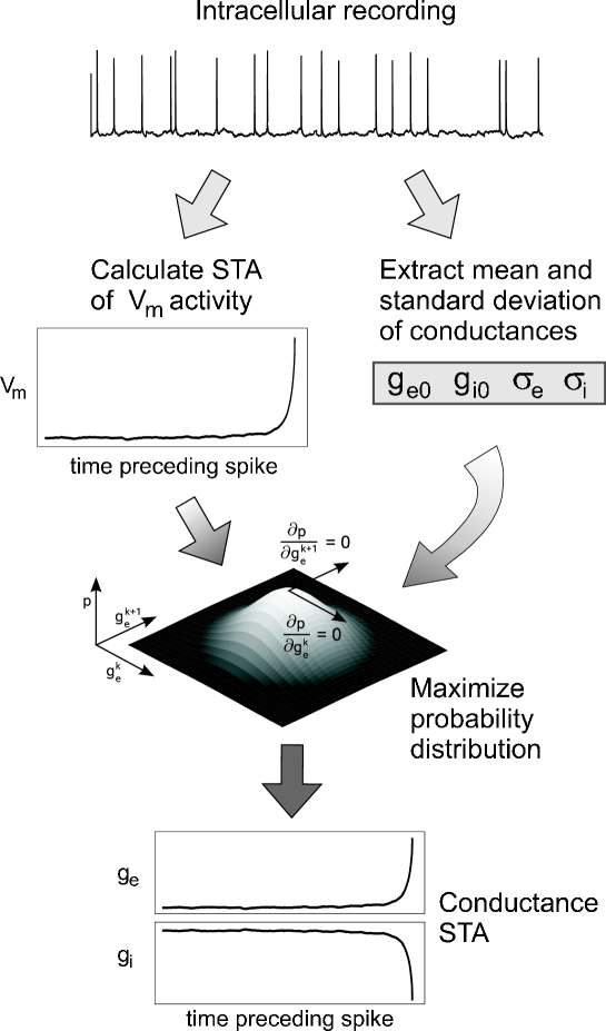
Figure 8: Scheme of the method to extract spike-triggered average conductances from membrane potential activity. Starting from an intracellular recording (top), the spike-triggered average (STA) membrane potential (V_m) is computed (leftmost panel). From the STA of the V_m, by discretizing the time axis, it is possible to estimate the STA of conductances (bottom) by maximizing a probability distribution (see text). This step requires knowledge of the values of the average conductances and their standard deviations ($g_{e0}$, $g_{i0}$, $\sigma_{e}$, $\sigma_{i}$, respectively), which must be extracted independently (rightmost panel).

Here, we have presented a method to extract the average excitatory and inhibitory conductance patterns directly related to spike initiation. As illustrated in Fig. 8, this method can extract spike-related conductances based solely on the knowledge of V_m activity. First, the STA of the V_m is computed from the intracellular recordings. Next, by discretizing the time axis, one estimates the “most likely” conductance time courses that are compatible with the observed STA of V_m. Due to the symmetry of their distribution, the average conductance time courses coincide with the most likely ones, so integration over the entire stimulus space (whose dimension depends on the STA interval as well as on the temporal resolution) can be replaced by a differentiation and subsequent solution of a system of linear equations. Solving this system gives an estimate of the average conductance time courses. We demonstrated that this estimation gives reasonably accurate estimates for the leaky IF model, as well as in real neurons under dynamic-clamp.

Like any other method, this method suffers from several sources of error. Errors can result from nonlinearities in the I-V curve of the neuron, e.g. those due to voltage-dependent conductances. In agreement with this, we have shown that the subthreshold activation of spike-generating currents close to threshold can lead to severe misestimations of the conductances (Fig. 4). This problem can be circumvented by excluding a short period (1–2 ms) preceding the spike. To avoid contamination by voltage-dependent currents, this method should be complemented by a check for I-V curve linearity in the range of V_m considered. Note that a linear I-V curve does not guarantee the absence of voltage-dependent conductances. For example, if the mean interspike interval of the cell becomes too short, spike-related potassium currents might be present during a substantial fraction of the STA interval and could affect the estimation. This might diminish the applicability of the method to neurons spiking at high frequency, in particular to fast-spiking interneurons. Also, strong subthreshold dendritic conductances that are very remote from the soma could influence the STA estimate without being visible in the I-V curve. On the other hand, in cases where it is possible to parameterize these nonlinearities, they can be included in Eq. 5. It should thus be possible to extend the method in order to apply it to more complex models, for example the exponential integrate-and-fire model (Fourcaud-Trocme et al., 2003). Another possible extension would be to include voltage-dependent terms such as N-methyl-D-aspartate (NMDA) receptor-mediated synaptic currents, although such currents probably have a limited contribution at the range of V_m considered here (below -50 mV).

Another source of error may arise from “negative conductances”. The present model of synaptic noise assumes that conductances are Gaussian-distributed, but if the standard deviation becomes comparable to the mean value of the conductances, the Gaussian distribution will include negative conductances, which are unrealistic. This is an important limitation of representing synaptic conductances by Gaussian-distributed noise (“diffusion approximation”). However, this type of approximation seems to apply well to cortical neurons in vivo, which receive a large number of inputs (Destexhe et al., 2001). In vivo measurements so far indicate that the standard deviation is much smaller than the mean for both excitatory and inhibitory conductances (Haider et al., 2006; Rudolph et al., 2005), which also indicates that the diffusion approximation is valid in this case. Such a check for consistency is a prerequisite for applying the present method.

Previous work related to the question of spike-triggered stimuli was mainly focused on white noise current inputs, and showed that no stable finite input average exists in the limit $dt\rightarrow 0$ (Paninski 2006a). Other contributions shed light on the question of membrane voltage STAs, for the leaky IF neuron as well as for biophysically more plausible models. However, so far no procedure was proposed to solve this problem of reverse correlation for conductance noise inputs. The method we propose here attempts to fill this gap, and directly provides a procedure that can be applied to real neurons. To this end, the present method must be complemented by measurements of the mean and standard deviation of excitatory and inhibitory conductances. Such measurements can be obtained either by voltage-clamp (Haider et al., 2006), or by current-clamp, as recently proposed (Rudolph et al., 2004, 2005). Combining the latter method with the present method, it should now be possible to directly extract conductance patterns from V_m recordings in vivo, and thus obtain estimates of the conductance variations related to spikes during natural network states.

References

Agüera y Arcas B. and Fairhall A. L. What causes a neuron to spike? Neural Computation 15: 1789-1807, 2003.

Badel L., Gerstner W. and Richardson M.J.E. Dependence of the spike-triggered average voltage on membrane response properties. Neurocomputing 69, 1062-1065, 2006.

Borg-Graham L., Monier C. and Frégnac Y. Visual input evokes transient and strong shunting inhibition in visual cortical neurons. Nature 393: 369-373, 1998.

de Boer F. and Kuypers P. Triggered Correlation. IEEE Trans. Biomed. Eng. 15: 169-197, 1968.

Destexhe A. and Rudolph M. Extracting information from the power spectrum of synaptic noise. J. Computational Neurosci. 17: 327-345, 2004.

Destexhe A., Rudolph M. and Paré D. The high-conductance state of neocortical neurons in vivo. Nature Reviews Neurosci. 4: 739-751, 2003.

Destexhe A., Rudolph M., Fellous J.-M. and Sejnowski T. J. Fluctuating synaptic conductances recreate in-vivo-like activity in neocortical neurons. Neuroscience 107: 13-24, 2001.

Fourcaud-Trocme N., Hansel D., van Vreeswijk C., Brunel N. How spike generation mechanisms determine the neuronal response to fluctuating inputs. J. Neurosci. 23(37): 11628-11640, 2003.

Haider B., Duque A., Hasenstaub A.R. and McCormick D.A. Network activity in vivo is generated through a dynamic balance of excitation and inhibition. J. Neurosci. 26: 4535-4545, 2006.

Hines M. L. and Carnevale N. T. (1997) The NEURON simulation environment. Neural Computation 9: 1179-1209, 1997

Monier C., Chavane F., Baudot P., Borg-Graham L. and Frégnac Y. Orientation and direction selectivity of synaptic inputs in visual cortical neurons: a diversity of combinations produces spike tuning. Neuron 37(4): 663-680, 2003.

Paninski L. The spike-triggered average of the integrate-and-fire cell driven by gaussian white noise. Neural Computation 18: 2592-2616, 2006a.

Paninski L. The most likely voltage path and large deviations approximations for integrate-and-fire neurons. J. Comput. Neurosci. 21: 71-87, 2006b.

Paninski L. , Pillow J. and Simoncelli E. Maximum likelihood estimation of a stochastic integrate-and-fire neural model. Neural Computation 16: 2533-2561, 2004.

Pillow J. and Simoncelli E. Biases in white noise analysis due to non-Poisson spike generation. Neurocomputing 52: 109-155, 2003.

Pinsky P. F. and Rinzel J. Intrinsic and network rhythmogenesis in a reduced Traub model for CA3 neurons. J. Comput. Neurosci. 1(1-2): 39-60, 1994.

Robinson H. P. and Kawai N. Injection of digitally synthesized synaptic conductance transients to measure the integrative properties of neurons. J. Neurosci. Methods 49(3): 157-165, 1993.

Rudolph M., Pelletier J.-G., Paré D. and Destexhe A. Characterization of synaptic conductances and integrative properties during electrically-induced EEG-activated states in neocortical neurons in vivo. J. Neurophysiol. 94: 2805-2821, 2005.

Rudolph M., Piwkowska Z., Badoual M., Bal T.. and Destexhe A. A method to estimate synaptic conductances from membrane potential fluctuations. J. Neurophysiol. 91: 2884-2896, 2004.

Sharp A. A., O’Neil M. B., Abbott L. F. and Marder E. The dynamic clamp: artificial conductances in biological neurons. Trends Neurosci. 16: 389-394, 1993.

Wehr M. and Zador A. Balanced inhibition underlies tuning and sharpens spike timing in auditory cortex. Nature 426 (6965):442-446, 2003.

Wilent W. and Contreras D. Dynamics of excitation and inhibition underlying stimulus selectivity in rat somatosensory cortex. Nature Neurosci. 8 (10):1364-1370, 2005.

Figure 2: The root-mean-square (RMS) of the deviation of the estimated from the recorded STAs. A: RMS deviation as a function of the number of spikes for the STA of excitatory conductance, where the SD of the conductance distribution was $10\%$ of its mean. The RMS deviation first decreases with the number of spikes, but saturates at $\sim 7000$ spikes. This is due to the effect of negative conductances, which are excluded in the simulation (cf. C). B: Same as A for inhibition. C: RMS deviation for excitation as a function of the ratio SD/mean of the conductance distribution. The higher the probability of negative conductances, the higher the discrepancy between theory and simulation. However, at SD/mean $=0.5$, the mean deviation is as low as $\sim 2\%$ of the mean conductance for excitation and $\sim 4\%$ for inhibition. D: Same as C for inhibition.