Coevolution. Extending
Prigogine theorem

Abstract.

The formal consideration of the concept of interaction in thermodynamic analysis makes it possible to deduce, in the broadest terms, new results related to the coevolution of interacting systems, irrespective of their distance from thermodynamic equilibrium. In this paper I prove the existence of privileged coevolution trajectories characterized by the minimum joint production of internal entropy, a conclusion that extends Prigogine theorem to systems evolving far from thermodynamic equilibrium. Along these trajectories of minimum internal entropy production one of the system goes always ahead of the other with respect to equilibrium.

1. Introduction

One of the primary objectives of non equilibrium thermodynamics is the analysis of open systems. As is well known, these systems maintain a continuous exchange (flow) of matter and energy with their environment. Through these flows, open systems organize themselves in space and time. However, the behaviour of such systems differs considerably according to whether they are close or far from equilibrium. Close to equilibrium the phenomenological relationships which bind the flows to the conjugate forces responsible for them are roughly linear, i. e. of the type:

$$J_{i}=\sum_{j}L_{ij}x_{j},\ i,j=1,2,\dots,n$$ (1)

where $J_{i}$ are the flows, $x_{j}$ the generalized forces, and $L_{ij}$ are the so called phenomenological coefficients giving the Onsager Reciprocal Relations [6, 7]:

$$L_{ij}=L_{ji},\ i\neq j$$ (2)

In these conditions, Prigogine’s Theorem [8] asserts the existence of states characterized by minimum entropy production. Systems can assimilate their own fluctuations and be self-sustaining.

Far from equilibrium, on the other hand, the phenomenology may become clearly non-linear, allowing the development of certain fluctuations that will reconfigure the system [1]. Thermodynamics of irreversible processes can now provide information regarding the stability of the system but not on its evolution. Far from equilibrium no physical potential exists capable of driving the evolution of systems [9]. The objective of the following discussion is just to derive certain formal conclusions related to that evolution in the case of interacting open systems evolving far from equilibrium.

2. Definitions

In the discussion that follow we will assume the following two basic assumptions:

1. There exist open systems whose available resources are limited.

2. Owing to these limitations, such systems compete with one another to maintain their necessary matter and energy flows.

Both assumptions lead directly to the concept of interaction. But before proposing a formal definition of that concept let us examine Figure 1 in order to obtain an intuitive idea of the type of problem being dealt with. Figure 1 provides a schematic representation of three open systems away from thermodynamic equilibrium. In the case (A) the system if not subjected to interaction with other systems, and maintains a through-flow of matter and energy which depends solely -without going into phenomenological details- on its own degree of imbalance. In the case (B) the systems interact with each other, and their respective flows depend on the degree of imbalance of both systems simultaneously. It is this situation which will be explored here as broadly as possible, particularly from the point of view of the coevolution of both systems.

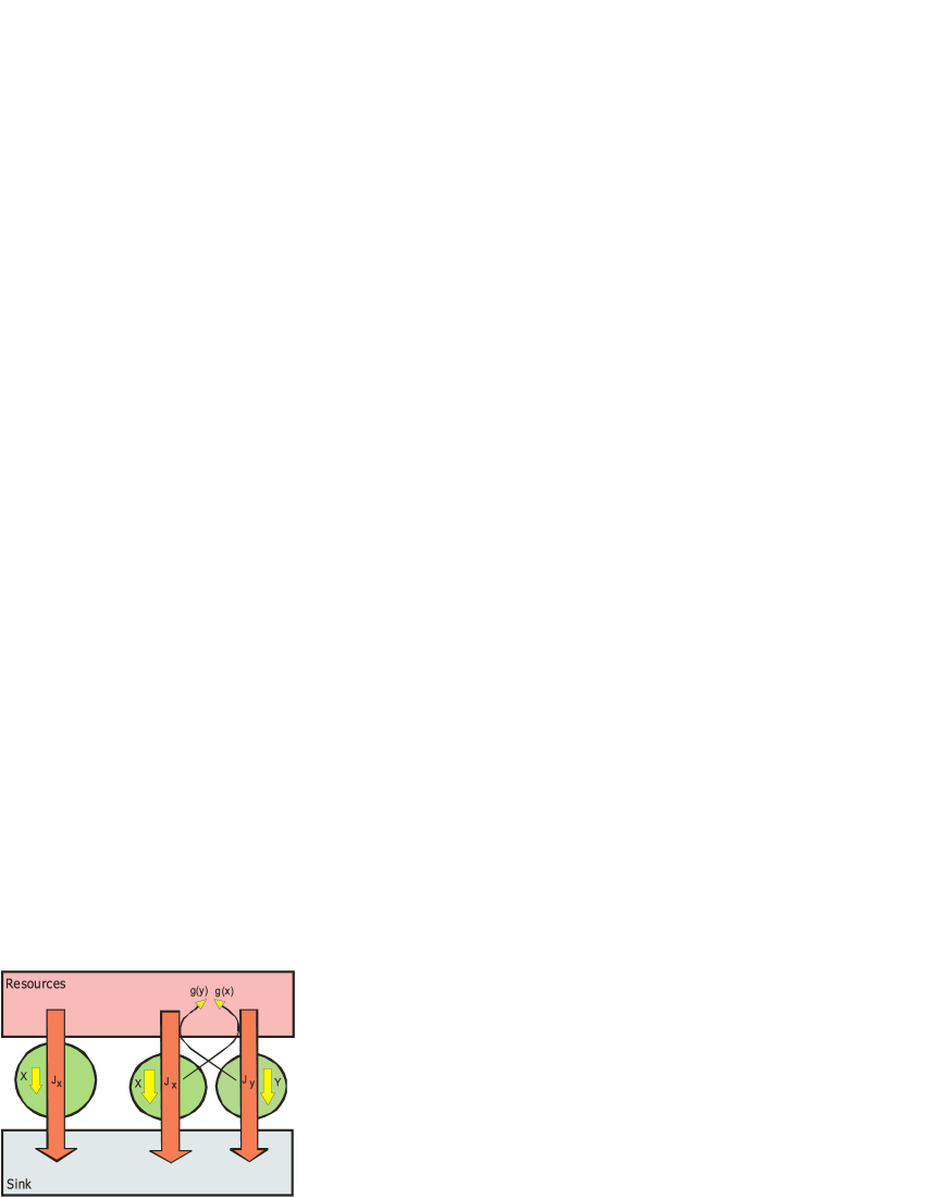
Figure 1. Circles represent open systems far from thermodynamic equilibrium. Rectangles represent significant parts of their environment (resources and sinks). Matter and energy flows are shown as large arrows crossing systems from resources to sinks. Yellow vertical arrows $x$ and $y$ represent the generalized forces responsible for the flows. Curved arrows $g(x)$ and $g(y)$ represent the interactions between the systems. In the absence of interaction with other systems, flows depend only on the intensity of the own force that maintain the system away from equilibrium ($J_{x}=f(x)$). When two systems compete with one another in order to maintain their flows, these flows depend on the intensity of the generalized forces (degree of imbalance) in both systems simultaneously. In these conditions, the flows are expressed by expression of the type $J_{x}=f(x)-g(y);J_{y}=f(y)-g(x)$ (see text).

Let $f$ and $g$ be any two type $\mathbb{C}^{2}$ functions (continuous functions with first and second derivatives which are also continuous functions) defined on the set $\mathbb{R}$ of real numbers and such as:

$$\text{$f$ and $g$ are strictly increasing, and }f(0)=g(0)=0$$ (3)

$$(f-g)$$ is strictly increasing (4)

$$(f-g)^{\prime}$$ is increasing. (5)

Function $f$ will be referred to as the phenomenological function and $g$ as the interaction function. The flow in a system will be given by $J_{x}=f(x)$ where $x$ is the generalized force, a measure of the degree of the system’s imbalance or distance from equilibrium. In consequence $x\geq 0$ ($x=0$ at equilibrium); $x$ will also be used to designate the system. Let us now justify the above constraints (3)-(5) on $f$ and $g$. Firstly, $f(0)=g(0)=0$ indicates that in the absence of generalized forces (thermodynamic equilibrium) there is neither flows nor interactions. The increasing nature of both functions indicate that the intensity of flows and interactions increase with the generalized forces, or in other words, as we move away from equilibrium. Constraints (4) and (5) imply that systems are progressively as sensitive to their own forces as they are to the forces of the other interacting system, or more so.

Given two systems with the same phenomenological function $f$ and forces $x$ and $y$ respectively, an interaction can be said to exist between them if their respective flows can be described by the following expressions:

$$J_{x}=f(x)+C_{xy}g(y),\ -1\leq C_{xy}\leq 1$$ (6)

$$J_{y}=f(y)+C_{yx}g(x),\ -1\leq C_{yx}\leq 1$$ (7)

where $C_{xy}$ and $C_{yx}$ are the interaction coefficients. We shall examine here the double negative, the positive-negative, and the double positive interaction, assuming -while still speaking in general terms- that $C_{xy}=C_{yx}=\pm 1$. Or in other words, that:

$$\begin{cases}J_{x}=f(x)\pm g(y)\\ J_{y}=f(y)\pm g(x)\end{cases}$$ (8)

In addition, the only $(x,y)$ pairs permitted will be those which give a positive value for expressions (8) above; $(x,y)$ pairs giving $f(x)-g(y)=0$ shall be termed the points of extinction of system $x$. The same applies to system y.

3. Entropy production

As is well known, the entropy balance for an open system can be expressed as:

$$dS=d_{i}S+d_{e}S$$ (9)

where $d_{i}S$ represents the entropy production within the system due to flows, and $d_{e}S$ is the entropy exchanged with its surroundings. The second law of thermodynamics dictates that always $d_{i}S\geq 0$ (zero only at equilibrium).

One of the most interesting aspects of Thermodynamics of Irreversible Processes is the inclusion of time in its equations:

$$\frac{d_{i}S}{dt}=\dot{S}_{i}=\sum_{j}x_{j}J_{j}$$ (10)

In our case, for system $x$ we have:

$$\frac{d_{ix}S}{dt}=\dot{S}_{ix}=x[f(x)-g(y)]\geq 0$$ (11)

and for system $y$:

$$\frac{d_{iy}S}{dt}=\dot{S}_{iy}=y[f(y)-g(x)]\geq 0$$ (12)

and the joint production of internal entropy:

$$\frac{d_{ix}S}{dt}+\frac{d_{ix}S}{dt}=\dot{S}(x,y)=x[f(x)-g(y)]+y[f(y)-g(x)]$$ (13)

Graphically $\dot{S}(x,y)$ is a surface in the space defined by the axes $\dot{S}$, $X$ and $Y$ (Figure 2). A curve in the plane $XY$ represents a possible coevolution history for both systems (as long as $x$ and $y$ satisfy (11) and (12)). Consequently, this type of curves will be termed as coevolution trajectories. The projection on the surface $\dot{S}(x,y)$ of a coevolution trajectory represents its cost in terms of internal entropy production. As we will immediately see, there exist special coevolution trajectories characterized by the minimum entropy production inside the systems evolving along them. They will be referred to as trajectories of minimum entropy (TME). Since the minimal entropy production inside the systems means the maximum regularity in their spacetime configurations, the points of a TME represents, states of maximum stability in systems interacting far away from thermodynamic equilibrium.

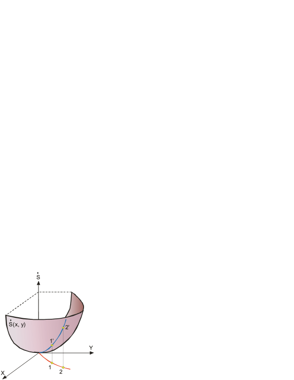
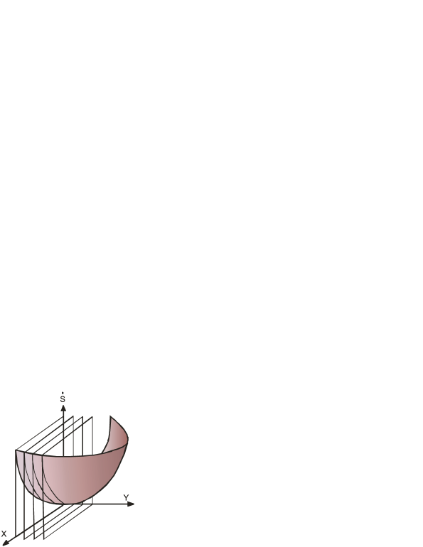
Figure 2. Left: Curve 1-2 represents any coevolutionary history between systems x and y. Curve 1’-2’, its projection on $\dot{S}(x,y)$, represents the joint production of internal entropy throughout that history. Right: Intersections of surface $\dot{S}(x,y)$ with the family of planes parallel to $\dot{S}X$.

We will now analyze surface $\dot{S}(x,y)$ for negative-negative, positive-negative and positive-positiveinteractions. And we will do it following a common mathematical method which consists in examining the intersections of the surface with one or more families of planes (Figure 2). In our case, three families will be used: the family of planes parallel to the plane $\dot{S}X$; the family of planes parallel to the plane $\dot{S}Y$; and the family of planes of the form $y=c-x$, which are perpendicular to the bisector $y=x$.

3.1. Negative-negative interaction

According to (8), in the case of a negative-negative interaction we will have:

$$\begin{cases}J_{x}=f(x)-g(y)\\ J_{y}=f(y)-g(x)\end{cases}$$ (14)

In these conditions, surface $\dot{S}(x,y)$ is given by:

$$\dot{S}(x,y)=x[f(x)-g(y)]+y[f(y)-g(x)]$$ (15)

Let us analyze its intersections with our three family of planes.

Planes parallel to $\dot{S}X$

Let $b$ be any real positive number. Consider the plane $y=b$. Its intersection with $\dot{S}(x,y)$ will be:

$$\dot{S}(x,b)=h(x)_{b}=x[f(x)-g(b)]+b[f(b)-g(x)]$$ (16)

If we derive $h(x)_{b}$ we will have:

$$\frac{d\dot{S}(x,b)}{dx}=h^{\prime}(x)_{b}=f(x)-g(b)+xf^{\prime}(x)-bg^{\prime}(x)$$ (17)

According to restrictions (3), (4) and (5), $h^{\prime}(x)_{b}$ is strictly increasing, and according to the same restrictions:

$$h^{\prime}(0)_{b}=-g(b)-bg^{\prime}(0)<0$$ (18)

$$h^{\prime}(b)_{b}=f(b)-g(b)+b[f^{\prime}(b)-g^{\prime}(b)]>0$$ (19)

Therefore, and in accordance with Bolzano’s theorem, there is a point $x_{b}$ such that:

$$h^{\prime}(x_{b})_{b}=0;\ 0<x_{b}<b$$ (20)

And, since $h^{\prime}(x)_{b}$ is strictly increasing, we have:

$$h^{\prime\prime}(x)_{b}>0;\ \forall x>0$$ (21)

Consequently $x_{b}$ is a minimum of $\dot{S}(x,b)$ (Figure 3)

So, the intersection of surface $\dot{S}(x,y)$ with the plane $y=b$ parallel to the plane $\dot{S}X$ is a curve $h(x)_{b}$ with a minimum. Or in other terms, for every $y>0$ there is a value of $x$ that minimizes the joint production of internal entropy in both systems. The couples $(x,y)$ satisfying this condition define a curve $T_{1}(x,y)$ in the plane $XY$ whose equation is:

$$f(x)-g(y)+xf^{\prime}(x)-yg^{\prime}(x)=0$$ (22)

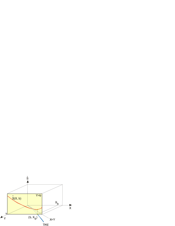
Figure 3. Intersection of surface $\dot{S}(x,y)$ with the plane $y=b$ parallel to the plane $\dot{S}X$.

which results from the fact that $h^{\prime}(x)_{y}=0$ for each $(x,y)$ in $T_{1}(x,y)$. Consequently, the couples $(x,y)$ satisfying (22) form a coevolution trajectory characterized by the minimal joint production of entropy inside the systems evolving along its points, that is to say a TME. According to (20), it holds the following St. Matthew inequality:

$$\forall(x,y)\in T_{1}(x,y):\ x<y$$ (23)

Note that according to the above reasoning this asymmetry is universal, independent of the particular functions $f$ and $g$, provided they verify constraints (3)-(5).

Planes parallel to $\dot{S}Y$

The same reasoning above now applied to the intersections of $\dot{S}(x,y)$ with planes parallel to $\dot{S}Y$ leads to a new coevolution trajectory $T_{2}(x,y)$ in the plane $XY$ whose equation is:

$$f(y)-g(x)+yf^{\prime}(y)-xg^{\prime}(y)=0$$ (24)

and whose points are also characterized by the minimal joint production of internal entropy in the systems evolving along them, i.e. A new TME. As in the case of $T_{1}(x,y)$, and for the same reasons, a new St. Matthew inequality holds:

$$\forall(x,y)\in T_{2}(x,y):\ y<x$$ (25)

Figure 4. Symmetry of the trajectories of minimum entropy production.

It is easy to see that $T_{1}(x,y)$ and $T_{2}(x,y)$ are symmetrical with respect to the bisector $y=x$. In fact, for $y=0$ equation (22) becomes:

$$f(x)+xf^{\prime}(x)=0$$ (26)

which only holds at $x=0$. The point (0, 0) belongs, therefore, to the trajectory. The same applies to (24). Consequently, the point (0,0), which corresponds to thermodynamic equilibrium, belongs to both trajectories. On the other hand, it is evident that:

$$T_{1}(x,y)=T_{2}(y,x)$$ (27)

Therefore, both trajectories are symmetrical with respect to the bisectrix $y=x$.

Intersections with planes of the form $y=c-x$

Let $c$ be any positive real number, the intersection of $\dot{S}(x,y)$ with the plane $y=c-x$ will be:

$$h(x)_{c-x}=x[f(x)-g(c-x)]+(c-x)[f(c-x)-g(x)]$$ (28)

whose derivative is

$$h(x)^{\prime}_{c-x}=f(x)-g(c-x)+xf^{\prime}(x)+xg^{\prime}(c-x)\\ -f(c-x)+g(x)-(c-x)f^{\prime}(c-x)-(c-x)g^{\prime}(x)$$ (29)

This derivative vanishes at point $x=c/2$:

$$h\left(\frac{c}{2}\right)^{\prime}_{c-x}=f\left(\frac{c}{2}\right)-g\left(\frac{c}{2}\right)+\frac{c}{2}f^{\prime}\left(\frac{c}{2}\right)+\frac{c}{2}g^{\prime}\left(\frac{c}{2}\right)\\ -f\left(\frac{c}{2}\right)+g\left(\frac{c}{2}\right)-\frac{c}{2}f^{\prime}\left(\frac{c}{2}\right)-\frac{c}{2}g^{\prime}\left(\frac{c}{2}\right)=0$$ (30)

And according to restrictions (3), (4):

$$h^{\prime\prime}\left(\frac{c}{2}\right)=4\left(f^{\prime}\left(\frac{c}{2}\right)+g^{\prime}\left(\frac{c}{2}\right)\right)+c\left(f^{\prime\prime}\left(\frac{c}{2}\right)-g^{\prime\prime}\left(\frac{c}{2}\right)\right)>0$$ (31)

we conclude that point $(c/2,c/2)$ is a minimum of the intersection $h(x)_{c-x}$. The same can be said of each point in the bisector $y=x$. In consequence, this line is a new trajectory of minimum entropy. It will be referred to as $T_{3}(x,y)$.

Figure 5. $\dot{S}(x,y)$ plotted in four sections orthogonal two by two. Each of those sections results from the intersection of $\dot{S}(x,y)$ with the planes $x=0$; $y=0$; $x=a$, $y=a$. A fifth section resulting from the intersection of $\dot{S}(x,y)$ with the plane $y=a-x$ has also been plotted.

The above results allow us to depict surface $\dot{S}(x,y)$ in the space defined by the axis $X$, $Y$ and $\dot{S}$ (Figure 5). Although the bisector $y=x$ is also a TME, it is not the most efficient in terms of entropy production. In effect, for each point $(b,b)$ of this line, two points $(x,b)$ and $(b,y)$ exist at which the interacting systems produce the less possible amount of internal entropy. The first of these points belong to $T_{1}(x,y)$, the second to $T_{2}(x,y)$ (Figure 6).

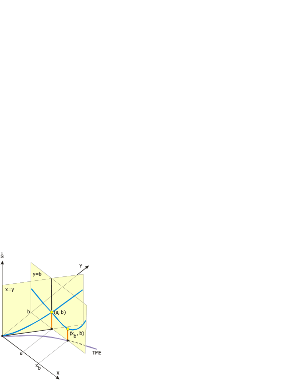
Figure 6. Although the bisector $y=x$ is also a TME, it is not the most efficient one in terms of internal entropy production.

As we have just seen, for each point $(a,b)$ of a coevolution trajectory, including the points of $T_{3}(x,y)$, there is a point $(x,b)$ in $T_{1}(x,y)$ and a point $(a,y)$ in $T_{2}(x,y)$ such that the joint entropy production inside the systems is the less possible one. This evidently applies to any point $(c,d)$ in the plane $XY$. In addition, and as a consequence of St. Matthew inequalities, one of the systems is always ahead of the other with respect to equilibrium. It holds therefore the following:

Theorem 1.

For every negative-negative interaction two trajectories of minimum entropy exist formed by a succession of states characterized by the minimum entropy production within the interacting systems. Furthermore, one of the systems is always ahead of the other with respect to thermodynamic equilibrium.

3.2. Positive-negative interaction

According to equations (6)-(7), and under the same restrictions of the negative-negative case, we will have now:

$$\begin{cases}J_{x}=f(x)+g(y)\\ J_{y}=f(y)-g(x)\end{cases}$$ (32)

The same considerations on the joint production of internal entropy we made in the case of the double negative interaction allow us now to express the entropy production in the positive-negative case as:

$$\frac{d_{ix}S}{dt}+\frac{d_{ix}S}{dt}=\dot{S}(x,y)=x[f(x)+g(y)]+y[f(y)-g(x)]$$ (33)

Again we have a surface $\dot{S}(x,y)$ which represents the joint entropy production inside the interacting systems. We will analyze it with the same intersection method.

Intersections parallel to $\dot{S}X$

The intersection of (33) with the plane $y=b$ is now:

$$h(x)_{b}=x(f(x)+g(b))+b(f(b)-g(x))$$ (34)

And its derivative:

$$h^{\prime}(x)_{b}=f(x)+g(b)+xf^{\prime}(x)-bg^{\prime}(x)$$ (35)

which is an strictly increasing function in accordance with the restrictions (3), (4) and (5). In addition, for $x=0$ equation (35) becomes:

$$h^{\prime}(0)_{b}=g(b)-bg^{\prime}(0)$$ (36)

While for $x=b$:

$$h^{\prime}(b)_{b}=f(b)+g(b)+b(f^{\prime}(b)-g^{\prime}(b))>0$$ (37)

Consequently, and according again to Bolzano’s theorem, if:

$$g(b)-bg^{\prime}(0)<0$$ (38)

there will be a point $x_{b}$ such that:

$$h^{\prime}(x_{b})_{b}=0$$ (39)

Taking into account that $h^{\prime}(x)_{b}$ is strictly increasing, we have:

$$h^{\prime\prime}(x)_{b}>0,\forall x>0$$ (40)

Therefore $x_{b}$ will be a minimum. Let us define $g_{1}(x)$ as $g(x)-xg^{\prime}(0)$. According to (38) there will be a trajectory of minimum entropy $T_{1}(x,y)$ if:

$$g_{1}(x)<0,\ \forall x>0$$ (41)

As in the case of the negative-negative interaction, its equation, will be:

$$f(x)+g(y)+xf^{\prime}(x)-yg^{\prime}(x)=0$$ (42)

Intersections parallel to $\dot{S}Y$

Let $a$ be any positive real number. The intersection of (33) with the plane $x=a$ is:

$$h(y)_{a}=a(f(a)+g(y))+y(f(y)-g(a))$$ (43)

and its derivative:

$$h^{\prime}(y)_{a}=ag^{\prime}(y)+f(y)-g(a)+yf^{\prime}(y)$$ (44)

which is a strictly increasing function according to restrictions (3), (4) and (5). For $y=0$ equation (44) becomes:

$$h^{\prime}(0)_{a}=ag^{\prime}(0)-g(a)$$ (45)

while for $y=a$ we have:

$$h^{\prime}(a)_{a}=(f(a)-g(a))+a(g^{\prime}(a)+f^{\prime}(a))>0$$ (46)

Therefore if:

$$ag^{\prime}(0)-g(a)<0$$ (47)

there will be a point $y_{a}$ such that:

$$h^{\prime}(y_{a})_{a}=0$$ (48)

Taking into account the strictly increasing nature of $h^{\prime}(y)_{a}$ we will have:

$$h^{\prime\prime}(y)_{a}>0,\ \forall y>0$$ (49)

Therefore $y_{a}$ will be a minimum. Let us define $g_{2}(x)$ as $xg^{\prime}(0)-g(x)$. According to (47) there will be a trajectory of minimum entropy $T_{1}(x,y)$ if:

$$g_{2}(x)<0,\ \forall x>0$$ (50)

Its equation will be:

$$f(y)-g(x)+yf^{\prime}(y)+xg^{\prime}(y)=0$$ (51)

Since

$$g_{1}(x)=g(x)-xg^{\prime}(0)$$ (52)

$$g_{2}(x)=xg^{\prime}(0)-g(x)$$ (53)

it is clear that:

$$g_{1}(x)=-g_{2}(x)$$ (54)

Both functions will only coincide at point $(0,0)$. In addition, if $g_{1}(x)<0$ then $g_{2}(x)>0$, and viceversa. Therefore, if $g_{1}(x)<0$ there exists $T_{1}(x,y)$, but not $T_{2}(x,y)$. Similarly, if $g_{2}(x)<0$ then there exists $T_{2}(x,y)$, but not $T_{1}(x,y)$. And since $xg^{\prime}(0)$ and $g(x)$ are two strictly increasing functions growing from $(0,0)$, it must exclusively hold one of those two alternatives; and then only one trajectory or minimum entropy, either $T_{1}(x,y)$ or $T_{2}(x,y)$, will exist.

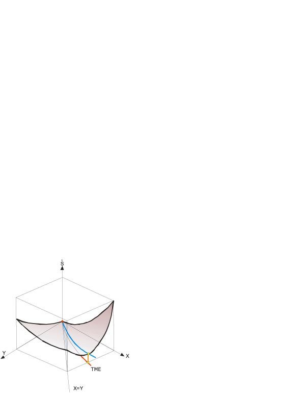
Figure 7. In the case of the positive-negative interaction, only a trajectory of minimum entropy exists.

Intersections with planes of the form $y=c-x$

Being $c$ any positive real number, the intersection of $\dot{S}(x,y)$ with the plane $y=c-x$ will be:

$$h(x)_{c-x}=x[f(x)+g(c-x)]+(c-x)[f(c-x))-g(x)]$$ (55)

and its derivative:

$$h^{\prime}(x)_{c-x}=f(x)+g(c-x)+xf^{\prime}(x)-xg^{\prime}(c-x)\\ -f(c-x)+g(x)-(c-x)f^{\prime}(c-x)-(c-x)g^{\prime}(x)$$ (56)

For $x=c/2$ we have:

$$h^{\prime}\left(\frac{c}{2}\right)_{c-x} =f\left(\frac{c}{2}\right)+g\left(\frac{c}{2}\right)+\frac{c}{2}f^{\prime}\left(\frac{c}{2}\right)-\frac{c}{2}g^{\prime}\left(\frac{c}{2}\right)$$

$$-f\left(\frac{c}{2}\right)+g\left(\frac{c}{2}\right)-\frac{c}{2}f^{\prime}\left(\frac{c}{2}\right)-\frac{c}{2}g^{\prime}\left(\frac{c}{2}\right)$$

$$=2g\left(\frac{c}{2}\right)-2\frac{c}{2}g^{\prime}\left(\frac{c}{2}\right)$$

Accordingly, the point $(c/2,c/2)$, and any other of the bisector $y=x$, will be a maximum or a minimum if:

$$g(x)=xg^{\prime}(x)$$ (57)

Point $(c/2,c/2)$ will be a minimum if:

$$h^{\prime\prime}(\frac{c}{2})=4f^{\prime}(\frac{c}{2})+c(f^{\prime\prime}(\frac{c}{2})>0$$ (58)

In this case the bisector $y=x$ is a TME. It will be referred to as $T_{3}(x,y)$. We have, then, three alternatives for the existence of TME in the case of positive-negative interactions:

$$\text{$T_{1}(x,y)$ exists if: }xg^{\prime}(0)>g(x)$$ (59)

$$\text{$T_{2}(x,y)$ exists if: }xg^{\prime}(0)<g(x)$$ (60)

$$\text{$T_{3}(x,y)$ exists if: }xg^{\prime}(x)=g(x)$$ (61)

$T_{3}(x,y)$ also requires condition (58).

As in the case of the double negative interaction, given a point $(a,b)$ of a coevolutionary trajectory, there exist either a point $(x,b)$ in $T_{1}(x,y)$ or a point $(a,y)$ in $T_{2}(x,y)$ such that the interacting systems produce the less possible amount of entropy inside the systems. Unlike the double negative interaction, in the positive-negative case only one TME exists. If that trajectory is:

$$f(x)+g(y)+xf^{\prime}(x)-yg^{\prime}(x)=0$$ (62)

it holds:

$$x=y\frac{g^{\prime}(x)}{f^{\prime}(x)}-\frac{f(x)}{f^{\prime}(x)}-\frac{g(y)}{f^{\prime}(x)}$$ (63)

According to restrictions (3)-(4)-(5), the first fraction is positive and less than 1, while the second and the third ones are positives. Therefore $x<y$, and system $y$ is always ahead of system $x$.

The other possible TME is:

$$f(y)-g(x)+yf^{\prime}(y)+xg^{\prime}(y)=0$$ (64)

whence:

$$y=\frac{g(x)-f(y)-xg^{\prime}(y)}{f^{\prime}(y)}$$ (65)

In accordance with restrictions (3)-(4)-(5), if $y>x$ the numerator would be negative, and being the denominator always positive, we would have a negative value for $y$, which is impossible (forces $x$ and $y$ are always positive). So $y$ is less than $x$. Consequently system $x$ is always ahead of system $y$. It holds, therefore, the following:

Theorem 2.

For every positive-negative interaction a trajectory of minimum entropy exists formed by a succession of states characterized by the minimum entropy production within the interacting systems. Furthermore, one of the systems is always ahead of the other with respect to thermodynamic equilibrium.

3.3. Positive-positive interaction

In the case of a double positive interaction, in the place of (8) we will have:

$$\begin{cases}J_{x}=f(x)+g(y)\\ J_{y}=f(y)+g(x)\end{cases}$$ (66)

and instead of (15):

$$\dot{S}(x,y)=x[f(x)+g(y)]+y[f(y)+g(x)]$$ (67)

Whence:

$$\frac{d\dot{S}(x,b)}{dx}=f(x)+g(b)+Xf^{\prime}(x)+bg^{\prime}(x)$$ (68)

$$\frac{d\dot{S}(a,y)}{dy}=f(y)+g(a)+Yf^{\prime}(y)+ag^{\prime}(y)$$ (69)

Both derivatives are positive, strictly increasing and only vanish at point $(0,0)$ corresponding to thermodynamic equilibrium. Intersections $\dot{S}(x,b)$, and for the same reasons intersections $\dot{S}(a,y)$, have neither maximums nor minimums.

The intersection of surface $\dot{S}(x,y)$ with the plane $y=c-x$ is now::

$$h(x)_{c-x}=x(f(x)+g(c-x))+(c-x)(f(c-x)+g(x)$$ (70)

and its derivative:

$$h^{\prime}(x)_{c-x}=f(x)+g(c-x)+xf^{\prime}(x)-xg^{\prime}(c-x)\\ -f(c-x)-g(x)-(c-x)f^{\prime}(c-x)+(c-x)g^{\prime}(x)$$ (71)

which vanishes at $x=c/2)$:

$$h^{\prime}\left(\frac{c}{2}\right)_{c-x} =f\left(\frac{c}{2}\right)+g\left(\frac{c}{2}\right)+\frac{c}{2}f^{\prime}\left(\frac{c}{2}\right)-\frac{c}{2}g^{\prime}\left(\frac{c}{2}\right)$$

$$-f\left(\frac{c}{2}\right)-g\left(\frac{c}{2}\right)-\frac{c}{2}f^{\prime}\left(\frac{c}{2}\right)+\frac{c}{2}g^{\prime}\left(\frac{c}{2}\right)=0$$

Therefore, there is a minimum at $x=c/2$ if the second derivative $h^{\prime\prime}(x)_{c-x}$ is positive. That is to say if:

$$2(f^{\prime}(x)-g^{\prime}(x))+x(f^{\prime\prime}(x)+g^{\prime\prime}(x))>0$$ (72)

In short, the only possible TME in the case of a double positive interaction is the bisectrix $y=x$. This conclusion together with the above two St. Matthew asymmetries allow us to state that stability in interacting systems requires either asymmetry or equality depending on the interaction nature: asymmetry for competition and equality for cooperation.

4. St. Matthew Theorem

’St Matthew Effect’ is the title of a paper by Robert k. Merton published in Science in the year 1968. The main objective of that paper was the analysis of the reward and communication systems of science. In its second page we can read: ”… eminent scientists get disproportionately great credit for their contributions to science while relatively unknown scientists tend to get disproportionately little credit for comparable contribution”. [5]. Or in other more general terms: the more you have the more you will be given, a pragmatic version of the so called St Matthew principle: ”For unto every one that hath shall be given, and he shall have abundance, but from him that hath not shall be taken away even that which he hath”. (St. Matthew 25:29). Sociologists, economists, ethologists and evolutionary biologists, among many others, had the opportunity to confirm the persistence of this St. Matthew asymmetry, which invariably appears in every conflict where any type of resource, including information, is at stake.

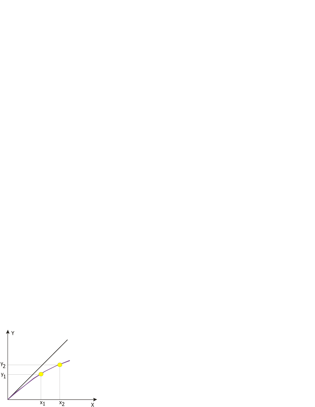
Figure 8. Systems evolving along a TME maintain an asymmetry related to their respective distance to thermodynamic equilibrium.

We have just proved, in the broadest terms, the existence of asymmetric coevolution trajectories for systems that interact according to certain formal definitions. These trajectories are thermodynamically relevant because their points represent states very far from equilibrium characterized by the minimum joint production of internal entropy in the interacting systems. Along these trajectories one of the system is always ahead of the other with respect to equilibrium. It has also been proved that those coevolution trajectories of minimum entropy exist if, and only if, at least one of the interactions is negative in the formal sense defined above. It has therefore been proved the following:

St Matthew theorem. For every binary interaction in which at least one of the interactions is negative, a coevolution trajectory exists characterized by the minimum joint production of internal entropy within the systems evolving along it, and such that one of the systems always goes ahead of the other with respect to thermodynamic equilibrium.

St Matthew theorem states, therefore, the same conclusion for systems far from thermodynamic equilibrium as Prigogine theorem for systems close to it.

5. Generalization

If we consider $n$ systems instead of 2, the following expressions would be obtained for flows:

$$J_{x_{i}}=f(x_{i})+\sum_{j}C_{ij}g(x_{j}),\ -1\leq C_{ij}\leq 1,\ i,j=1,2,\dots n$$ (73)

where $C_{ij}$ represents (as the binary case) the type and degree of interaction between systems $x_{i}$ and $x_{j}$. The joint production of internal entropy could thus be expressed as:

$$\dot{S}(x_{1},x_{2},\dots x_{n})=\sum_{i}X_{i}\left[f(x_{i})+\sum_{j}C_{ij}g(x_{j})\right]$$ (74)

where $\dot{S}(x_{1},x_{2},\dots x_{n})$ is a hypersurface on $\mathbb{R}^{n+1}$ in which we can consider $\sum(n-1)$ three-dimensional subspaces $\dot{S}x_{i}X_{j}$ in order to analyze the interaction between the system $x_{i}$ and the system $x_{j}$ using the same method as in the binary case.

6. Discussion

The most relevant feature of an open system is its ability to exchange matter and energy with its environment. But not all processes involved in those exchanges are equally efficient. Far form equilibrium, systems are subjected to the non linear dynamic of fluctuations. In those conditions, the most efficient process are those that generate the lower level of internal entropy because the excess of entropy may promote an excess of fluctuations driving the system towards instability. We have proved the existence of coevolution trajectories whose most remarkable characteristic is just the minimum level of internal entropy production. The states of the systems evolving along those trajectories are, therefore, the most efficient ones in terms of self maintenance. In these conditions and taking into account the tremendous competence and selective pressure suffered by many systems, as is the case of the biological or the economical systems, the trajectories of minimum entropy should be taken as significant references. They in fact represent histories of maximum stability in open systems interacting very far from thermodynamic equilibrium, which is very a common situation in the real world. Apart from its own existence, it is remarkable the asymmetrical way the systems evolve along them (St Matthew theorem). A result compatible with the empirical observations of evolutionary biology that biologists know long time ago and that is usually referred to as St Matthew principle [4]. It is also confirmed by a recent experimental research related to recursive interactions by means of logistic functions [3].

References

- [1] P. Glansdorff and I. Prigogine, Structure, Stabilité et Fluctuations, Mason, Paris, 1971.
- [2] Antonio León Sánchez, Coevolution: New Thermodynamic Theorems, Journal of Theoretical Biology 147 (1990), 205 – 212.
- [3] Antonio Leon, Beyond chaos. introducing recursive logistic interactions, http://arxiv.org/abs/0804.3057v1, 2008.
- [4] R. Margalef, La Biosfera, entre la termodinámica y el juego., Omega, Barcelona, 1980.
- [5] Robert K. Merton, The Matthew Effect in Science, Science 159 (1968), 56–33.
- [6] Lars Onsager, Reciprocal relations In Irreversible processes I, Phys. Rev. 37 (1931), 405 – 426.
- [7] by same author, Reciprocal relations in irreversible Processes Ii, Phys. Rev. 38 (1931), 2265 – 2279.
- [8] Ilya Prigogine, Étude thermodynamique des Phénomènes irréversibles, Bull. Acad. Roy. Belg. 31 (1945), 600.
- [9] H. V. Volkenshtein, Biophysics, MIR, Moscow, 1983.