A Multiscale Model of Biofilm as a Senescence-Structured Fluid

Abstract

We derive a physiologically structured multiscale model for biofilm development. The model has components on two spatial scales, which induce different time scales into the problem. The macroscopic behavior of the system is modeled using growth-induced flow in a domain with a moving boundary. Cell-level processes are incorporated into the model using a so-called physiologically structured variable to represent cell senescence, which in turn affects cell division and mortality. We present computational results for our models which shed light on modeling the combined role senescence and the biofilm state play in the defense strategy of bacteria.

1 Introduction

In this paper we derive a physiologically structured multiscale model for biofilm development. The model has components on two spatial scales, which induce different time scales into the problem. The macroscopic behavior of the system is modeled using growth-induced flow in a domain with a moving boundary, following [1, 11] . Cell-level processes are incorporated into the model using a so-called physiologically structured variable to represent cell senescence, which in turn affects cell division and mortality. We use “senescence” to mean “the organic process of growing older and showing the effects of increasing age”.

The multiscale nature of physiologically and spatially structured population models, such as those in this paper and in [3, 6, 12, 13], differs from more typical multiscale systems where the smaller spatial scales have the faster time scales. In the structured multiscale systems, the dynamics of the relevant physiology of individuals within a population are homogenized to a distribution of a representative trait, such as age, size or senescence. Although the underlying physiological system may have a very fast time scale (such as the protein network within a cell that controls the cell cycle), the distribution of the representative trait may evolve relatively slowly compared to the dynamics in space or in the reaction terms (such as the age distributions used to represent a tumor cell’s position in the cell cycle in [6], or a Proteus mirabilis multinuclear filament cell’s length in [3, 12]).

The derivation of the model in this paper follows that of Alpkvist and Klapper [1], with the addition of the explicit physiological structure in the bacteria populations based on the notion of bacteria senescence demonstrated in [23] for cells with symmetric division and [8, 20] for cells with asymmetric division. We also include explicit tracking of inert cell populations, which includes necrotic cells.

To our knowledge, prior to this work, physiological structure has only been integrated into spatial models where motion is due to migration or taxis, represented by diffusion terms in the model equations [3, 6, 12, 13]. Here, instead, motion is driven by growth-induced expansive stress, a much different mechanism that requires inclusion of a force balance equation.

This paper is organized as follows. We first motivate the problem subject and derive the structured multiscale model of biofilm growth. Following this, we present a nondimensionalization and then a spatially homogeneous steady-state age distribution, which in combination help to illustrate the differing age structures occurring in different places in the biofilm. Finally, we provide computational results for our models which shed light on the combined role senescence, and the self-organization into a biofilm state, play in the defensive capabilities of bacteria.

2 Biofilms and Age Dependence

A biofilm is a collection of microorganisms, typically bacteria, enclosed within a self-secreted polymeric matrix. These films are generally attached on one side to a solid boundary and, on the other, access substrates (e.g. oxygen) through a free surface, Figure 1. See [24] for a review. Biofilm properties change over long times (weeks) – it is possible to describe a maturation process in the development of a particular biofilm. That is, biofilms demonstrate aging effects. We are thus motivated to extend basic biofilm models to include age dependence.

In fact, it seems that individual bacteria themselves suffer age dependence in the form of senescence. This property had been observed for some time in asymmetric dividers [8, 20]; more recently senescence has also been noted in the symmetric divider Escherichia coli [23]. Under normal conditions, senescent cells make up a small percentage of the total population. However, aging (over medium time scales) may provide an effective defense against short time scale environmental disruptions but without affecting microbial community vitality during normal conditions. That is, we posit that multi-time scale behavior allows a powerful defense mechanism. In a recent paper [17], it was argued that cell senescence offers a simple explanation for the phenomenon of bacterial persistence. Bacteria exhibit the phenomenon of “persistence”, the tendency for a small number of cells within a larger population to tolerate a wide range of antimicrobial challenges [7, 14, 16]. In particular, the mechanism for this tolerance was suggested to be that senescent cells were less active and hence less susceptible than younger, more vigorous ones. Then, once the antimicrobial attack ceases, the persisting cells could produce new, vital cells which in turn would be capable of regenerating the colony. Previously, others have argued that persisters were phenotypic variants [7, 10, 19, 21, 22].

Colony defense through persister cells is likely to be especially effective in biofilms where surviving persister cells, though perhaps small in number, have the opportunity to be protected by the biofilm matrix [19]. As a result of this matrix they may have a particularly conducive environment for re-population once the antimicrobial challenge has ended. Thus, in order to demonstrate that senescent cells can distribute themselves throughout the biofilm and as a particular application of our age dependent biofilm model, we compute the spatial and temporal variation of age dependence. These senescent cells are produced on a medium time-scale (approximately 1 day): fast relative to the biofilm maturation time but slow compared to metabolic times. Thus persisters are generated quickly enough so that they can be an effective defense mechanism for mature biofilms but not so quickly that they interfere with competitive fitness.

3 Derivation of the Model

We consider a spatial domain $\Omega$ consisting of stratified subdomains $B_{t}$ for biomass and $\Omega\backslash B_{t}$ for the bulk fluid. There are two moving interfaces in $\Omega$: $\Gamma_{t}$ separating $B_{t}$ from the rest of $\Omega$, and a bulk-substrate interface $\Gamma_{H_{b}}$ that is a fixed height $H_{b}$ above $\Gamma_{t}$. The biofilm rests on a surface, denoted by a lower boundary, $\Gamma_{B}$. The spatial domains are illustrated in Figure 1.

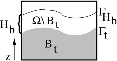
Fig. 1: Spatial domains for the senescence-structured biofilm model.

We let $b_{i}(t,{\bf x},a)$, $i=1,\ldots,N_{b}$, denote the densities of the bacteria phenotypes in time $t\geq 0$, space ${\bf x}\in B_{t}$, and senescence $a\geq 0$, and let ${\bf J}_{i}^{b}$ denote their respective fluxes. The component of ${\bf x}$ representing height is denoted by $z$. Similarly, $c_{i}(t,{\bf x})$, $i=1,\ldots,N_{c}$, denote the substrate concentrations in time $t\geq 0$ and space ${\bf x}\in\Omega$, and ${\bf J}_{i}^{c}$ denotes their respective fluxes. In addition to active cell types, we allow for the presence of inert cells, including necrotic cells, that do not use or produce substrates, do not grow, and are not merely in a quiescent state. Lack of senescence allows us to list these separately from the $b_{i}$ because these cells do not have any age dependence. We let $n_{i}(t,{\bf x})$ denote inert cells of type $b_{i}$ of all ages, and ${\bf J}_{i}^{n}$ their respective fluxes.

Conservation of biomass yields equations

$$\frac{\partial b_{i}}{\partial t}+\frac{\partial(g_{i}(a,c_{1},\ldots,c_{N_{c}})\,b_{i})}{\partial a}+\nabla\cdot{\bf J}_{i}^{b}\\ =-\hat{\mu}_{i}(a,c_{1},\ldots,c_{N_{c}},b_{1}(t,{\bf x},\cdot),\ldots,b_{N_{b}}(t,{\bf x},\cdot))b_{i}(t,{\bf x},a)\\ +\hat{f_{i}}(b_{1}(t,{\bf x},a),\ldots,b_{N_{b}}(t,{\bf x},a)),$$ (1)

for $i=1,\ldots,N_{b}$ where $\hat{\mu}_{i}$ is the inactivation or “death” modulus with dependence on senescence, substrate concentrations and the densities of all bacteria phenotypes of all ages, and $\hat{f}_{i}$ is the rate of net change to phenotypes $i$ from all other phenotypes. The terms $\hat{f}_{i}$ allows the possibility that bacteria have the capability of changing their phenotype in response to stimuli. A model that incorporated change due to mutation would do so in the age boundary condition. The senescence rate $g_{i}$ represents the physical wear-and-tear experienced by an aging individual in response to nutrient and/or oxygen uptake and exposure to waste.

Due to the close relationship between senescence and chronological age, for this paper we make the simplifying assumption that $g_{i}\equiv 1$, for $i=1,\ldots,N_{b}$. Further below, we will specify senescence as a function of age for use in both the inactivation modulus, $\hat{\mu}$, and the fecundity, $\hat{\beta}$, defined below. Equations (1) then become the age- and space-structured equations

$$\frac{\partial b_{i}}{\partial t}+\frac{\partial b_{i}}{\partial a}+\nabla\cdot{\bf J}_{i}^{b}\\ =-\hat{\mu}_{i}(a,c_{1},\ldots,c_{N_{c}},b_{1}(t,{\bf x},\cdot),\ldots,b_{N_{b}}(t,{\bf x},\cdot))b_{i}(t,{\bf x},a)\\ +\hat{f_{i}}(b_{1}(t,{\bf x},a),\ldots,b_{N_{b}}(t,{\bf x},a)).$$ (2)

Observations in [23] showed that even in symmetric cell division, one of the two new cells contains older material and overall less vitality than the other (referred to as “old pole” and “new pole” cells, resp.). This results in a physiologically structured mathematical representation of the bacterial cell cycle that is closer to that for birth-death processes in animals than what has been commonly used to represent cell division [6, 25]. These models were built on the assumption that a mother cell divided into two daughter cells of equal and high vitality, thereby assigning each daughter cell a senescence of zero and removing the mother cell from the population. In our old-pole/new-pole formulation rather, the mother cell remains in the population and continues to undergo senescence from the point it had at cell division while giving rise to a single daughter cell with senescence zero. This notion of senescence allows two implications, based on the account in [23], that are relevant to the model in this paper. First, old-pole cells grow slower than new-pole cells produced in the same division. Second, old-pole cells become inert at a higher rate than new-pole cells.

Although a more elaborate model would include explicit size structure similar to what was done in models in [6, 25], we can take advantage of continuous senescence and time to incorporate the first old-pole/new-pole issue into a fecundity term, $\hat{\beta}_{i}(a,c_{1},\ldots,c_{N_{c}},b_{1}(t,{\bf x},\cdot),\ldots,b_{N_{b}}(t,{\bf x},\cdot))$, with dependence on age, substrate concentrations and the densities of all bacteria phenotypes of all ages. Differences in individual sizes influence volume fractions, represented by giving mother cells with larger offspring a corresponding higher fecundity. The fecundities, $\hat{\beta}$, account not just for differences in daughter size due to the mother’s size, but also heterogeneities in the mean growth rates across phenotypes $i$. A third more minor property of cell senescence mentioned in [23], that new-pole cells are marginally more likely to divide sooner than old-pole cells, can also be included in $\hat{\beta}$. (Similarly, we can incorporate the second property of higher incidence of becoming inert into $\hat{\mu}_{i}$.) The resulting senescence boundary condition, or “birth” condition, is

$$b_{i}(t,{\bf x},0)=\int_{0}^{\infty}\hat{\beta}_{i}(a,\ldots)b_{i}(t,{\bf x},a)\ da,\qquad\mbox{for }i=1,\ldots,N_{b}.$$ (3)

We represent retention of inert cells using $N_{b}$ inert-cell classes governed by the conservation equations

$$\frac{\partial n_{i}(t,{\bf x})}{\partial t}+\nabla\cdot{\bf J}_{i}^{n}=\int_{0}^{\infty}\hat{\mu}_{i}(a,\ldots)b_{i}(t,{\bf x},a)\ da,\qquad\mbox{for }i=1,\ldots,N_{b}.$$ (4)

Conservation of substrate mass yields

$$\frac{\partial c_{i}}{\partial t}+\nabla\cdot{\bf J}_{i}^{c}=r_{j},\qquad\mbox{for }j=1,\ldots,N_{c},$$ (5)

where $r_{j}$ denotes gain or loss of the $j$-th substrate concentration through interactions with the biomass such as consumption or excretion. Assuming Fick’s Law gives ${\bf J}_{j}^{c}=-D_{j}\nabla c_{j}$ for constants $D_{j}$. The substrate masses are also subject to advection, but the velocity is sufficiently slow that we can neglect the advective contribution to the flux. Likewise, substrate material diffuses several orders of magnitude faster than the rates at which bacteria grow or advect, allowing us to make a quasi-steady-state assumption so that

$$-D_{j}\nabla^{2}c_{j}=r_{j},\qquad\mbox{for }j=1,\ldots,N_{c}.$$ (6)

We let $\vartheta_{i}(t,{\bf x},a)$ and $\rho_{i}(t,{\bf x},a)$ denote the volume fraction per age and density per age relative to volume fraction, resp., of phenotypes $i$, so that $b_{i}=\rho_{i}\theta_{i}$. We assume incompressibility of biomass with $\rho_{i}(t,{\bf x})\equiv\rho^{*}_{i}$ for positive constants $\rho_{i}^{*}$. We also assume inert cells have the same incompressibility properties, and the same densities relative to volume fractions, $\rho_{i}^{*}$, as active cells. We let $\eta_{i}(t,{\bf x})$ denote the volume fraction of inert phenotype $i$ cells, which is related to the density of inert phenotype $i$ cells by $n_{i}=\rho_{i}^{*}\eta_{i}$. We assume such cells all behave the same regardless of phenotype, and track only the total volume fraction of inert cells of all phenotypes, denoted by $\mathcal{N}(t,{\bf x})$. Equations (4), rewritten as

$$\frac{\partial\eta_{i}(t,{\bf x})}{\partial t}+\frac{1}{\rho_{i}^{*}}\nabla\cdot{\bf J}_{i}^{n}=\int_{0}^{\infty}\mu_{i}(a,\ldots)\vartheta_{i}(t,{\bf x},a)\ da,\qquad\mbox{for }i=1,\ldots,N_{b},$$ (7)

become, after summing over $i$, the governing equation for $\mathcal{N}$,

$$\frac{\partial\mathcal{N}(t,{\bf x})}{\partial t}+\sum_{i=1}^{N_{b}}\frac{1}{\rho_{i}^{*}}\nabla\cdot{\bf J}_{i}^{n}=\mathcal{M}(t,{\bf x}),$$ (8)

where

$$\mathcal{N}(t,{\bf x}) = \sum_{i=0}^{N_{b}}\eta_{i}(t,{\bf x}),$$ (9)

$$\mathcal{M}(t,{\bf x}) = \sum_{i=0}^{N_{b}}\int_{0}^{\infty}\mu_{i}(a,\ldots)\vartheta_{i}(t,{\bf x},a)\ da.$$ (10)

We require the biomass volume fractions to total to one so that

$$\mathcal{N}(t,{\bf x})+\sum_{i=1}^{N_{b}}\int_{0}^{\infty}\vartheta_{i}(t,{\bf x},a)\ da=1.$$ (11)

Assuming that transport of biomass, including inert cells, is governed by an advective process, with a volumetric flow ${\bf u}(t,{\bf x})$ for all classes and ages, gives the fluxes ${\bf J}_{i}^{b}=\rho^{*}_{i}\vartheta_{i}{\bf u}$ for $i=1\ldots,N_{b}$. Following [1, 11], we assume that the volumetric flow is stress driven according to

$${\bf u}=-\lambda\nabla p,$$ (12)

where $p(t,{\bf x})$ is the pressure and $\lambda>0$ the Darcy constant. As in [1, 11], $p=0$ in $\Omega\backslash B_{t}$. Pressure is determined in order to enforce incompressibility in response to growth (see below) and hence (12) can be viewed as a balance of growth-induced stress against friction. Other choices of force balance are possible.

Substituting $b_{i}=\rho_{i}^{*}\vartheta_{i}$ and ${\bf J}_{i}^{b}=\rho^{*}_{i}\vartheta_{i}{\bf u}$ into equations (2) gives, for $i=1,\ldots,N_{b}$,

$$\frac{\partial\vartheta_{i}}{\partial t}+\frac{\partial\vartheta_{i}}{\partial a}+\nabla\cdot({\bf u}\vartheta_{i})=-\mu_{i}(a,c_{1},\ldots,c_{N_{c}},\vartheta_{1}(t,{\bf x},\cdot),\ldots,\vartheta_{N_{b}}(t,{\bf x},\cdot))\vartheta_{i}(t,{\bf x},a)\\ +f_{i}(\vartheta_{1}(t,{\bf x},a),\ldots,\vartheta_{N_{b}}(t,{\bf x},a)),$$ (13)

where

$$\mu_{i}(a,c_{1},\ldots,c_{N_{c}},\vartheta_{1}(t,{\bf x},\cdot),\ldots,\vartheta_{N_{b}}(t,{\bf x},\cdot))=\\ \hat{\mu}_{i}(a,c_{1},\ldots,c_{N_{c}},b_{1}(t,{\bf x},\cdot),\ldots,b_{N_{b}}(t,{\bf x},\cdot))$$ (14)

and

$$f_{i}(\vartheta_{1}(t,{\bf x},a),\ldots,\vartheta_{N_{b}}(t,{\bf x},a))=\frac{1}{\rho_{i}^{*}}\hat{f}_{i}(b_{1}(t,{\bf x},a),\ldots,b_{N_{b}}(t,{\bf x},a)).$$ (15)

The birth conditions (3) become

$$\vartheta_{i}(t,{\bf x},0)=\int_{0}^{\infty}\beta_{i}(a,\ldots)\vartheta_{i}(t,{\bf x},a)\ da,\qquad\mbox{for }i=1,\ldots,N_{b}.$$ (16)

where

$$\beta_{i}(a,c_{1},\ldots,c_{N_{c}},\vartheta_{1}(t,{\bf x},\cdot),\ldots,\vartheta_{N_{b}}(t,{\bf x},\cdot))=\\ \hat{\beta}_{i}(a,c_{1},\ldots,c_{N_{c}},b_{1}(t,{\bf x},\cdot),\ldots,b_{N_{b}}(t,{\bf x},\cdot)).$$ (17)

Substituting ${\bf J}_{i}^{n}=\rho^{*}_{i}\eta_{i}{\bf u}$ into equation (8) and using equation (9) gives

$$\frac{\partial\mathcal{N}}{\partial t}=\mathcal{M}-\nabla\cdot{\bf u}\mathcal{N},$$ (18)

Integrating equation (13) over age and summing over $i$ gives

$$\underbrace{\frac{\partial}{\partial t}\left(\sum_{i=1}^{N_{b}}\int_{0}^{\infty}\vartheta_{i}(t,{\bf x},a)\ da\right)}_{=\nabla\cdot({\bf u}\mathcal{N})-\mathcal{M}}+\underbrace{\left(\sum_{i=1}^{N_{b}}\int_{0}^{\infty}\frac{\partial\vartheta_{i}(t,{\bf x},a)}{\partial a}\ da\right)}_{=-\mathcal{B}\mbox{ as defined below}}=\\ -\underbrace{\nabla\cdot\left({\bf u}\sum_{i=1}^{N_{b}}\int_{0}^{\infty}\vartheta_{i}(t,{\bf x},a)\ da\right)}_{=\nabla\cdot({\bf u}(1-\mathcal{N}))}-\underbrace{\left(\sum_{i=1}^{N_{b}}\int_{0}^{\infty}\mu_{i}(a,\ldots)\vartheta_{i}(t,{\bf x},a)\ da\right)}_{=\mathcal{M}}\\ +\underbrace{\left(\sum_{i=1}^{N_{b}}\int_{0}^{\infty}f_{i}(\vartheta_{1}(t,{\bf x},a),\ldots,\vartheta_{N_{b}}(t,{\bf x},a))\ da\right)}_{=\mathcal{F}\mbox{ as defined below}}.$$ (19)

Using equations (11) and (18), we find that the first term in the first line of equation (19) is $\partial_{t}(1-\mathcal{N})=\nabla\cdot({\bf u}\mathcal{N})-\mathcal{M}$. For the second term in the first line, we assume that $\vartheta_{i}$, for $i=1,\ldots,N_{b}$, are sufficiently smooth, and that the corresponding $\mu_{i}$ are bounded away from zero for $a$ large, so that each $\vartheta_{i}$ will eventually decay exponentially to zero as $a\rightarrow\infty$ (see section 7 in [2]). We then obtain for the negative of the second term, using the age boundary conditions defined by equation (16),

$$\mathcal{B}(t,{\bf x}) = \sum_{i=0}^{N_{b}}\vartheta_{i}(t,{\bf x},0)$$ (20)

$$= \sum_{i=0}^{N_{b}}\int_{0}^{\infty}\beta_{i}(a,\ldots)\vartheta_{i}(t,{\bf x},a)\ da.$$

For the first term in the second line of equation (19), we again use equation (11) to obtain $\nabla\cdot({\bf u}(1-\mathcal{N}))$. Recall that the second to last term of equation (19) is just $\mathcal{M}(t,{\bf x})$ and set the last term to

$$\mathcal{F}(t,{\bf x})=\sum_{i=0}^{N_{b}}\int_{0}^{\infty}f_{i}\ da.$$ (21)

We note that $\mathcal{F}$ is not generally identically zero; a similar sum over all phenotypes of the integrals over all ages of the net changes between phenotypes, $\hat{f}$, is conserved to be zero. However, because the densities relative to volume fractions, $\rho_{i}^{*}$, are not identical, we generally only have $\mathcal{F}\equiv 0$ when $\rho_{i}^{*}=\rho^{*}$ for some constant $\rho^{*}$ and for all $i=1,\ldots,N_{b}$. We rewrite equation (19) more compactly as

$$\nabla\cdot{\bf u}=\mathcal{B}(t,{\bf x})+\mathcal{F}(t,{\bf x}),$$ (22)

the incompressibility relation for our system.

Substituting ${\bf u}=-\lambda\nabla p$ results in an equation for the pressure, namely

$$-\lambda\nabla^{2}p=\mathcal{B}(t,{\bf x})+\mathcal{F}(t,{\bf x}),\qquad\mbox{in }B_{t}.$$ (23)

Distributing the divergence operator, and again using ${\bf u}=-\lambda\nabla p$ along with equation (22), gives us $\nabla\cdot({\bf u}\vartheta_{i})=-\lambda\nabla p\cdot\nabla\vartheta_{i}+\vartheta_{i}(\mathcal{B}+\mathcal{F})$, so that equation (13) can be rewritten, for $i=1,\ldots,N_{b}$,

$$\frac{\partial\vartheta_{i}}{\partial t}+\frac{\partial\vartheta_{i}}{\partial a}-\lambda\nabla p\cdot\nabla\vartheta_{i}=-\mu_{i}\vartheta_{i}+f_{i}-\vartheta_{i}(\mathcal{B}+\mathcal{F}),$$ (24)

Similarly, we rewrite equation (18) as

$$\frac{\partial\mathcal{N}}{\partial t}=\mathcal{M}+\lambda\nabla p\cdot\nabla\mathcal{N}-\mathcal{N}(\mathcal{B}+\mathcal{F}).$$ (25)

We see from equation (23) that $p$ is proportional to $\lambda^{-1}$, so that $\lambda\nabla p$ is independent of $\lambda$. Consequently, $\vartheta_{i}$ and $\mathcal{N}$ are independent of $\lambda$, allowing us to set $\lambda=1$.

We impose periodic and other boundary conditions similar to what was done in [1] to obtain the complete model, for $i=1,\ldots,N_{b}$ and $j=1,\ldots,N_{c}$,

$$\frac{\partial\vartheta_{i}}{\partial t}+\frac{\partial\vartheta_{i}}{\partial a}-\nabla p\cdot\nabla\vartheta_{i}=-\mu_{i}\vartheta_{i}+f_{i}-\vartheta_{i}(\mathcal{B}+\mathcal{F}),\qquad{\bf x}\in B_{t},t>0,a>0,$$ (26a)

$$\vartheta_{i}(t,{\bf x},0)=\int_{0}^{\infty}\beta_{i}(a,\ldots)\vartheta_{i}(t,{\bf x},a)\ da,\qquad {\bf x}\in B_{t},t>0,$$ (26b)

$$\frac{\partial\vartheta_{i}}{\partial z}=0,\qquad {\bf x}\in\Gamma_{B},t\geq 0,a>0,$$ (26c)

$$\vartheta_{i}(0,{\bf x},a)=\vartheta_{i}^{0}({\bf x},a),\qquad {\bf x}\in B_{t},a\geq 0,$$ (26d)

$$\frac{\partial\mathcal{N}}{\partial t}-\nabla p\cdot\nabla\mathcal{N}=\mathcal{M}-\mathcal{N}(\mathcal{B}+\mathcal{F}),\qquad {\bf x}\in B_{t},t>0,$$ (26e)

$$\frac{\partial\mathcal{N}}{\partial z}=0,\qquad {\bf x}\in\Gamma_{B},t\geq 0,$$ (26f)

$$\mathcal{N}(0,{\bf x})=\mathcal{N}^{0}({\bf x}),\qquad {\bf x}\in B_{t},$$ (26g)

$$-\nabla^{2}p=\mathcal{B}+\mathcal{F},\qquad {\bf x}\in B_{t},t\geq 0,$$ (26h)

$$p=0,\qquad {\bf x}\in\Gamma_{t},t\geq 0,$$ (26i)

$$\frac{\partial p}{\partial z}=0,\qquad {\bf x}\in\Gamma_{B},t\geq 0,$$ (26j)

$$-D_{j}\nabla^{2}c_{j}=r_{j},\qquad {\bf x}\in\Omega,t>0,$$ (26k)

$$r_{j}=0,\qquad {\bf x}\in\Omega\backslash B_{t},$$ (26l)

$$c_{j}=c_{j}^{*},\qquad {\bf x}\in\Gamma_{H_{b}},t\geq 0,$$ (26m)

$$\frac{\partial c_{j}}{\partial z}=0,\qquad {\bf x}\in\Gamma_{B},t\geq 0.$$ (26n)

The normal velocity of the interface $$\Gamma_{B}$$ is given by

$$-\nabla p\cdot{\bf n}=-\frac{\partial p}{\partial n},$$ (26o)

where $${\bf n} \Gamma_{B}$$ is the unit outward normal of .

We make particular choices of functions $\beta$ and $\mu$ as follows. To reflect the diminished new-cell production by senescent cells discussed in [23], we define senescence as a function of age, $\sigma(a)$, such that $\sigma(0)=0$ and $\sigma(a)\rightarrow 1$ as $a\rightarrow\infty$, and incorporate $\sigma(a)$ into $\beta(a,c)$ and $\mu(a,c)$,

$$\beta(a,c) =\beta_{0}(c)\left(1-\sigma(a)\right),$$ (27a)

$$\mu(a,c) =\mu_{0}(c)\sigma(a).$$ (27b)

We neglect the $c$ dependence of $\mu_{0}$, and choose

$$\sigma(a) =\frac{a}{a^{*}+a},\qquad a\geq 0,$$ (28a)

$$\beta_{0}(c) =\frac{\psi\,c}{k+c},$$ (28b)

where $a^{*}$ is the senescence age scale, and, following [1], $\psi$ is the maximum growth rate (with units of inverse age) and $k$ is the Monod saturation constant (with units of concentration). Oxygen uptake has the form

$$r(c,\vartheta(t,{\bf x},\cdot))=\frac{\xi\,c}{k+c}\int_{0}^{\infty}(1-\sigma(a))\vartheta(t,{\bf x},a)\ da,$$ (29)

where $\xi$ is the maximum uptake rate.

4 Non-dimensionalization

We simplify in the following to $N_{b}=N_{c}=1$, i.e., restrict to one active phenotype and one substrate, and drop indexing subscripts. Note now that $\mathcal{N}=\eta(t,{\bf x})$ and $\mathcal{M}=\int_{0}^{\infty}\mu(a,\ldots)\vartheta(t,{\bf x},a)\,da$. Also note that $f=\mathcal{F}=0$. We will continue to assume that $\beta=\beta(a,c)$ and $\mu=\mu(a,c)$.

Let $\bar{\beta}$ be a typical value of $\beta(a,c)$ and let $\bar{\mu}$ be a typical value of $\mu(a,c)$. Choosing a characteristic time scale $T=1/\bar{\beta}$, age scale $A=1/\bar{\mu}$, and temporarily reintroducing the friction coefficient $\lambda$, we nondimensionalize according to $\tilde{t}=t/T$, $\tilde{a}=a/A$, $\tilde{x}=x/L$, and $\tilde{\beta}=\beta T$, $\tilde{\mu}=\mu A$, $\tilde{c}=c/c^{*}$, $\tilde{r}=r/r(c^{*})$, $\tilde{p}=p(\lambda T/L^{2})$, $\tilde{\vartheta}=\vartheta A$, $\tilde{\eta}=\eta$. Here $L$ is a (problem-dependent) characteristic system length scale.

Substituting into the system (26) and dropping tildes, we obtain

$$\frac{\partial\vartheta}{\partial t}+\Lambda\frac{\partial\vartheta}{\partial a}-\nabla p\cdot\nabla\vartheta=-\Lambda\mu\vartheta-\vartheta\int_{0}^{\infty}\beta(a,c)\vartheta(a)\,da,\qquad{\bf x}\in B_{t},t>0,a>0,$$ (30a)

$$\vartheta(t,{\bf x},0)=\int_{0}^{\infty}\beta(a,c)\vartheta(t,{\bf x},a)\ da,\qquad {\bf x}\in B_{t},t>0,$$ (30b)

$$\frac{\partial\vartheta}{\partial z}=0,\qquad {\bf x}\in\Gamma_{B},t\geq 0,a>0,$$ (30c)

$$\vartheta(0,{\bf x},a)=\vartheta_{0}({\bf x},a),\qquad {\bf x}\in B_{t},a\geq 0,$$ (30d)

$$\frac{\partial\eta}{\partial t}-\nabla p\cdot\nabla\eta=\Lambda\int_{0}^{\infty}\mu(a,c)\vartheta(a)\,da-\eta\int_{0}^{\infty}\beta(a,c)\vartheta(a)\,da,\quad{\bf x}\in B_{t},t>0,$$ (30e)

$$\frac{\partial\eta}{\partial z}=0,\qquad {\bf x}\in\Gamma_{B},t\geq 0,$$ (30f)

$$\eta(0,{\bf x})=\eta_{0}({\bf x}),\qquad {\bf x}\in B_{t},$$ (30g)

$$\nabla^{2}p=-\int_{0}^{\infty}\beta(a,c)\vartheta(a)\,da,\qquad {\bf x}\in B_{t},t\geq 0,$$ (30h)

$$p=0,\qquad {\bf x}\in\Gamma_{t},t\geq 0,$$ (30i)

$$\frac{\partial p}{\partial z}=0,\qquad {\bf x}\in\Gamma_{B},t\geq 0,$$ (30j)

$$\nabla^{2}c=-Gr,\qquad {\bf x}\in\Omega,t>0,$$ (30k)

$$r=0,\qquad {\bf x}\in\Omega\backslash B_{t},$$ (30l)

$$c=1,\qquad {\bf x}\in\Gamma_{H_{b}},t\geq 0,$$ (30m)

$$\frac{\partial c}{\partial z}=0,\qquad {\bf x}\in\Gamma_{B},t\geq 0.$$ (30n)

Here $G=L^{2}r(c^{*})/(c^{*}D)$ and thus $1/\sqrt{G}$, the active layer depth, is a non-dimensional measure of the depth (scaled by system size) to which substrate can penetrate into the biofilm before it is consumed. Likewise

$$\Lambda=\frac{\bar{\mu}}{\bar{\beta}}$$ (31)

is a non-dimensional ratio of characteristic deactivity time to characteristic reproduction time.

The non-dimensional forms of equations (28a) and (28b) are

$$\sigma(a) =\frac{a}{S+a},\qquad a\geq 0,$$ (32a)

$$\beta_{0}(c) =\frac{P\,c}{K+c},$$ (32b)

where $S=a^{*}/A$ is a comparison of senescence age with system age scale, $K=k/c^{*}$ is a measure of saturation level (large $K$ means substrate-limited behavior and small $K$ indicates growth-limited behavior), and $P=\psi/\bar{\beta}$ is a measure of maximum to typical yield.

The magnitude of $\Lambda$ may depend on location within the biofilm. We identify two regimes. First, near the top of the biofilm, in particular within the active layer, $c$ is ${\mathcal{O}}(1)$ and we can then generally expect for a viable biofilm that $\bar{\beta}$ be large compared to $\bar{\mu}$, i.e., $\Lambda$ small. In this case advective terms dominate in equations (30a) and (30e) over the death terms. If advection is unimportant, i.e., $\nabla p\cdot\nabla\vartheta$ is small, then age scale is determined by the second term of (30a) which then requires $\partial/\partial a\sim\Lambda^{-1}$. Such scaling is in fact observed within the biofilm active layer, see Section 6.

Second, beneath the active layer, equation (30k) indicates exponential decay (in space) of $c$. Hence, below a sharp transition region from the active layer, we can expect $\bar{\beta}$ to be small compared to $\bar{\mu}$, i.e., $\Lambda$ large. In this case at first glance equation (30a) indicates $\vartheta$ has an $\mu$-governed decaying age structure. There is a subtlety here however. Large $\Lambda$ in (30a) suggests an approximately exponential age profile of the form $\vartheta(a)=\vartheta(0)\exp(-\mu a)$. But such a form is inconsistent with (30b), which does not allow dependence on $\mu$, unless $\vartheta(0)=0$. In other words, for large $\Lambda$ the birth term is insufficient to introduce enough new cells to overcome death and so an active population is not viable. Having said this, however, we will observe a $\mu$-determined exponential age structure develop in the deeper parts of the biofilm, see Section 6. The reason for this is that in the lower layer of the biofilm, where the population is barely viable, the birth rate has decreased to the point that it is only just balancing death. Hence condition (30b), which requires that an exponential age structure be controlled by $\beta$, also implies that exponential age structure be determined by $\mu$.

5 Spatially Homogeneous Steady-State Age Distributions

We assume spatial homogeneity and temporal stationarity, i.e., $\vartheta=\vartheta(a)$, $\eta=\eta(a)$, on $-\infty<z<\infty$. (We note that pressure gradients within the biofilm and hence advection are generally weak within inactive regions.) Then $\vartheta$, $\eta$ satisfy

$$\frac{d\vartheta}{da} = -(\mu+\vartheta_{0})\vartheta,$$ (33)

$$\vartheta_{0} = \int_{0}^{\infty}\beta\vartheta\,da,$$ (34)

$$\eta = 1-\int_{0}^{\infty}\vartheta(a)\,da,$$

where $\vartheta_{0}=\vartheta(0)$. This system is unphysical in that it requires unbounded velocities (the pressure gradient takes the form $p_{z}=C_{1}z+C_{2}$) to enforce incompressibility, but it is nevertheless useful for illustrative purposes.

The solution to equation (33) is

$$\vartheta(a)=\vartheta_{0}e^{-\int_{0}^{a}\mu\,da^{\prime}}e^{-\vartheta_{0}a}.$$ (35)

Thus equation (34) implies the condition

$$\vartheta_{0}=\int_{0}^{\infty}\beta\vartheta_{0}e^{-\int_{0}^{a}\mu\,da^{\prime}}e^{-\vartheta_{0}a}\,da.$$ (36)

In order to have a nontrivial solution, we require $\vartheta_{0}$ to satisfy

$$1=\int_{0}^{\infty}\beta e^{-\int_{0}^{a}\mu\,da^{\prime}}e^{-\vartheta_{0}a}\,da,$$ (37)

if possible. If this is not possible, then $\vartheta_{0}=\vartheta(a)=0$ is the only solution.

The choice of $\mu$ and $\beta$ independent of $a$ allows a particular transparence. In this case condition (37) becomes

$$1=\int_{0}^{\infty}\beta e^{-(\mu+\vartheta_{0})a}\,da,$$ (38)

which has a solution with $\vartheta_{0}>0$ if

$$\int_{0}^{\infty}\beta e^{-\mu a}\,da>1,$$ (39)

i.e., if new cells can be produced sufficiently fast to replace aging (and dying) ones. Note that this condition cannot be satisfied for $\mu$ sufficiently large or $\beta$ sufficiently small (in which case $\vartheta_{0}=0$ necessarily). Now if we write $\vartheta_{0}=\hat{\vartheta}_{0}-\mu$, then $\hat{\vartheta}_{0}$ solves

$$1=\int_{0}^{\infty}\beta e^{-\hat{\vartheta}_{0}a}\,da,$$ (40)

that is, $\hat{\vartheta}_{0}=\beta$. Equation (35) becomes

$$\vartheta(a)=(\beta-\mu)e^{-\beta a}.$$ (41)

Fecundity $\beta$ fixes the profile of the age structure though age distribution amplitude depends on both $\beta$ and $\mu$. Large $\beta$ results in a steep age profile with amplitude almost independent of $\mu$. Small $\beta$ results in a flat age profile. However we note that the viability boundary (in parameter space) occurs at $\beta=\mu$. For marginally viable populations $\beta=\mu+\epsilon$ and hence the population age profile is exponential with decay rate approximately $\mu$. Note that $\mu$ gives the slowest possible rate of decay. With regards to a biofilm model, if we assume that $\beta$ decreases with decreasing $c$, then age structure should flatten deeper down into the biofilm. In fact, we expect an abrupt transition from steep to flat profile as we pass through the active layer.

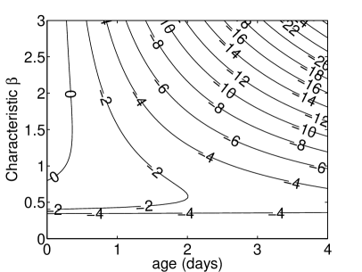
(a) Response of $\ln(\theta(a))$ to changes in $\bar{\beta}$.

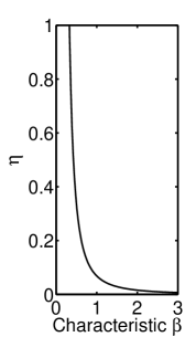
(b) Response of $\eta$ to changes in $\bar{\beta}$.

Fig. 2: Response of steady-state solutions to changes in the characteristic reproduction rate, $\bar{\beta}=\int_{0}^{a^{*}}\beta(a,c)\,da$.

Returning to our specified forms of $\beta(a,c)$ and $\mu(a,c)$ we have

$$\vartheta(a) =\vartheta(0)\left(\frac{S}{a+S}\right)^{-\mu_{0}(1)S}e^{-\mu_{0}(1)a}e^{-\vartheta(0)a/\Lambda},$$ (42a)

$$\eta =\Lambda\frac{\mu_{0}(1)}{\vartheta(0)}\int_{0}^{\infty}\frac{a}{a+S}\vartheta(a)\,da.$$ (42b)

Going back for a moment to dimensional variables, we use days as units of time, take $\mu_{0}=0.25$, and vary $\beta_{0}(c)$ to induce changes in a characteristic reproduction rate, $\bar{\beta}=\int_{0}^{a^{*}}\beta(a,c)\,da$. We set $a^{*}=0.5$, which accounts for a loss of 1% vitality per division (occurs on average every 0.02 days for E. coli). Figure 2 shows the response of the steady-state solutions to changes in $\bar{\beta}$. We note that the steady-state active-cell distribution is zero when $\bar{\beta}$ is less than roughly 0.33.

6 Computational Results

In this section we present computational results for one spatial dimension (height of the biofilm), and explicit age structure representing cell senescence, for the dimensional system (26). The height of the biofilm, $\Gamma_{t}$, is regulated using an erosion term at the biofilm/substrate interface (a standard devise in biofilm models, see e.g. [15]) given by

$$\frac{\partial\Gamma_{t}}{\partial t}=-\frac{\partial p}{\partial z}\bigg{|}_{z=\Gamma_{t}}-\alpha\Gamma_{t}^{2},$$ (43)

where $\alpha$ is the erosion coefficient.

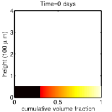
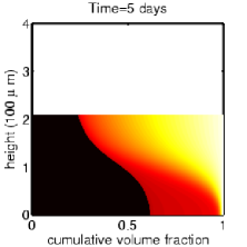
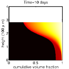
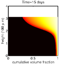
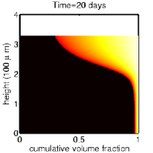
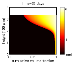
Fig. 3: Biofilm dynamics from initial colonization to steady state. The height of the colored area represents the height of the biofilm, including both active and inert bacteria. Color represents cell state: black represents inert cells, and a spectrum from off-white to yellow to orange to red represents senescence of a cell of a given age, $\sigma(a)$. The horizontal width of a color constitutes the volume fraction of cells of the corresponding senescence.

For the computations presented in this section, we consider again the case of $N_{b}=N_{c}=1$. We take as the initial condition a biofilm with a height of $\Gamma_{t}(0)=50\mu\mbox{m}$ and with an age distribution that is initially the same for all heights, $\vartheta(0,z,a)=0.35*\max(1-\frac{a}{4},0)$ for $0\leq z\leq 50\mu\mbox{m}$. This piecewise linear function, when converted from age structure to senescence structure (recall $\sigma(a)=\frac{a}{a^{*}+a}$) , closely approximates the senescence structure at the top of the biofilm when it is near steady state and thus represents a situation where a new area is being colonized by material from the top of a mature biofilm when it is near steady state. The motivation is that a young biofilm may be formed by colonization of cells detached from the upper region of an upstream, mature biofilm.

We use a time unit equal to one day. As a result, we take the senescence time scale to be $a^{*}=0.5$, as was done in Section 5. We use the division time for E. coli, which is roughly every 30 minutes.

We set the erosion parameter to be $\alpha=0.03$, the distance between $\Gamma_{t}$ and $\Gamma_{H_{b}}$ to be $H_{b}=37.5\mu\mbox{m}$, and the parameters for the various functional forms to be $\mu_{0}=0.25$, $k=0.05$, $\psi=2$, $\xi=3$, and $c^{*}=1$. These parameter values are of the same order of magnitude of those used in [1], with modifications due to the inclusion of age structure in the model equations.

Results of the computations with the above parameters are displayed in Figure 3. The height of the colored area indicates the height of the biofilm, including both active and inert bacteria. Color represents cell state: black designates inert cells, and a spectrum from off-white to yellow to orange to red designates senescence of a cell of a given age, $\sigma(a)$. The horizontal width occupied by a color indicates the volume fraction of cells of the corresponding senescence.

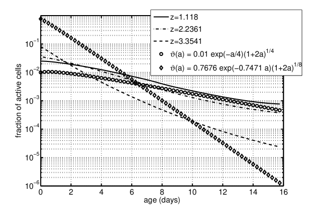
Fig. 4: Normalized age distributions, ignoring the inert cell populations, one third of the way from the bottom, two thirds of the way from the bottom, and at the top of the biofilm at time $t=25$ days. The plot of $\vartheta(a)=0.01\,\exp(-a/4)(1+2a)^{1/4}$ is the large $\Lambda$ limit of equation (42a). The coefficient of 0.01 governing the magnitude of the curve is chosen for ease of comparison. The plot of $\vartheta(a)=0.7676\,\exp(-0.7471\,a)(1+2a)^{1/8}$ is the re-normalized steady-state, given an oxygen concentration of $c=0.5581$, in the absence of advection. Differences between this curve and the computed solution at the top of the biofilm illustrate the role of advection, including the upward flow of a relatively greater proportion of inert and senescent cells

The biofilm tends to a steady state, as discussed in Section 5, consisting of an active layer at the top and passive layer appearing as a stalk. It is already understood that this physical structure provides a form of protection for the bacteria population as a whole [9]. The question remains: how does senescence and the corresponding resistance to antimicrobial challenge fit into the overall defensive strategy of bacteria?

To obtain an answer, we first consider the normalized age distributions, ignoring the inert cell populations, one third of the way from the bottom, two thirds of the way from the bottom, and at the top of the biofilm at time $t=25$ days. These distributions are shown in Figure 4.

As we descend the biofilm down through the active layer and into the passive layer, we expect $\Lambda$ to increase so that equation (30a) approaches, in steady state, equation 42a. The plot of $\vartheta(a)=0.01\,\exp(-a/4)(1+2a)^{1/4}$ highlights the convergence toward the shape of the curve of the large $\Lambda$ limit of equation (42a). The coefficient of 0.01 governing the magnitude of the curve is chosen for ease of comparison. At the top of the biofilm at steady-state, the oxygen concentration is approximately $c=0.5581$. Using this value, our specific functional forms defined in equations (27)-(28), and equations (35) and (37), we obtain a value of $\theta_{0}=0.6221$. We re-normalize the age distribution to total one so that equation (35) has the specific form $\vartheta(a)\approx 0.7676\,\exp(-0.7471\,a)(1+2a)^{1/8}$. This represents the situation when there is no advection. Differences between this function and the graph of the computed steady-state age distribution at the top of the biofilm reflect the role of advection, including the upward flow of material with a relatively higher proportion of inert and senescent cells.

We find the expected result, as discussed in Sections 4 and 5, that the age distributions broaden as we go from the active to the passive layers within the biofilm. In the inactive region, the profile matches that of an approximately growth-death balanced population. This is to be expected in an erosion maintained steady state – some growth must occur all the way to the bottom of the biofilm. A non-viable zone does not form in the presence of erosion because such a zone does not result in any growth induced pressure and hence does not increase expansive velocity. We remark that it is possible that $\mu$-dominated age structure in the inactive region of the biofilm is thus a byproduct of erosion. A more general (and realistic) biofilm model would allow for the possibility of mechanical detachment; this would require a much more elaborate set-up than the one used here (i.e., mechanical stress coupling in three dimensions). It is still plausible that a non-viable zone would lead to detachment and so we posit that age structure would not change.

Finally, we extend the computation to include the effects of antimicrobial challenge. We assume the antimicrobial agent has a source at the bulk-substrate interface $\Gamma_{H_{b}}$, that it diffuses on a fast time scale compared to growth, and, for simplicity, that it is not degraded by the biofilm. Consequently, the antimicrobial saturates the biofilm essentially instantaneously and thus we can model the effects of antimicrobial challenge by modifying the death modulus $\mu$ rather than adding an additional chemical species equation to our system:

$$\mu(t,a,c)=\mu_{0}\sigma(a)+\mu_{1}(t,c)(1-\sigma(a)).$$ (44)

This form assumes that older cells are more resistant to antimicrobial challenge than younger cells, and that the antimicrobial agent affects metabolically active cells more than less active cells, represented by the oxygen dependence of $\mu_{1}$. In particular, we take

$$\mu_{1}(t,c)=\left\{\begin{array}[]{rl}\frac{50c}{k+c},&\qquad 35\leq t\leq 35.2,\\ 0,&\qquad\mbox{otherwise.}\end{array}\right.$$ (45)

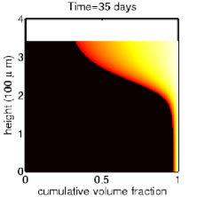
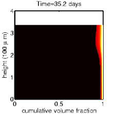
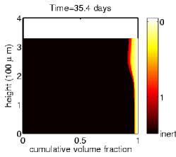
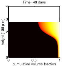
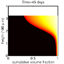
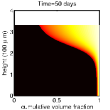
Fig. 5: Response to an antimicrobial agent applied from time $t=35$ to time $t=35.2$. The height of the colored area represents the height of the biofilm, including both active and inert bacteria. Color represents cell state: black represents inert cells, and a spectrum from off-white to yellow to orange to red represents senescence of a cell of a given age, $\sigma(a)$. The horizontal width of a color constitutes the volume fraction of cells of the corresponding senescence.

Results are shown in Figure 5 for the case when an antimicrobial agent is applied from time $t=35$ to time $t=35.2$. The senescence structure of the population in the stalk allows it to maintain itself even after the active layer is largely decimated. Moreover, upon removal of the antimicrobial agent, the population of older cells in the active layer is quickly replaced by younger cells, which then return the biofilm to its steady state over a longer maturation time. Note that the height continues to drop after removal of the antimicrobial agent prior to regrowth.

6.1 Numerical Methods

We employ a moving-grid Galerkin method in age, using piecewise constants as the approximation space [2]. The use of higher-order approximation spaces in age was discussed in [4]. The moving-grid Galerkin method decouples the age and time discretizations, while allowing age and time to advance together along characteristic lines. Consequently, we are able to solve the model equations in age without numerical dispersal or oscillations. Because the transport in age is computed by the movement of the grid, rather than by a difference approximation of the age derivative or through jump terms in a standard discontinuous Galerkin method, the only meaningful source of error is approximation error, which underlies the superconvergence results in [2, 4]. For the case of piecewise constant functions, we obtain a second-order correct method in age.

We integrate time using a step-doubling method [5]. Step-doubling consists of taking one step of backward Euler over a time step, and then taking two half steps of backward Euler over the same time interval. This results in two things. First, we can compare the two late-time solutions for the error control needed for the adaptivity in time. Second, we can extrapolate the two solutions to get a likely second-order accurate solution in time.

For the spatial variable, we discretize, over a uniform partition, the domain $[0,\Gamma_{t}]$ and compute the changes in biofilm height by solving equation (43). We impose a boundary condition on $c$ at $\Gamma_{t}$ by using a ghost node positioned at $\Gamma_{H_{b}}$. Fluxes are computed using upwind differencing [18]. Although this method is only first-order correct, it has been sufficient for the computations presented in this paper, given the lack of sharp fronts in the interior of the biofilm, $[0,\Gamma_{t}]$. More advanced methods will be needed for computations with more spatial dimensions.

The discretizations in the computational results presented above used a uniform partition of the spatial interval $[0,\Gamma_{t}]$ with 301 nodes, and a uniform age discretization of the truncated age domain, $[0,16]$, with $\Delta a=1/8$ and piecewise constant basis functions. A uniform age discretization in the context of the moving-grid Galerkin method means that all but the first and last age intervals are constant in length, and that a new age interval is introduced at the birth boundary when the old birth interval reaches $\Delta a$ in length. The tolerance parameter for the adaptive time-stepping in the step-doubling algorithm was $5\times 10^{-3}$.

7 Conclusions

In this paper we presented a multiscale model and simulation of biofilm development that is interesting for three major reasons. One is the nonstandard multiscale nature of the problem: cell division and aging is a result of complex, and fast, micro- and nano-scale processes, at least when compared to the advective scale of the biofilm growth. However, by representing the cell division and aging process using notions of senescence and age, we have a mechanism for the cellular scale that, in keeping with what has been observed in other age- and space-structured multiscale systems [3, 6, 12, 13], is in general slower than the advective process. But even here we see novelty; unlike [3, 6, 12, 13], the relative ranking of the time scales of the aging and advective processes inverts as we move from an active layer at the top of the biofilm to a passive layer below. Further, both of these times scales are fast with respect to the biofilm maturation time.

This inversion of the time scales underlies another major point of interest: the implication that the active layer does not merely provide a physical shield for a reservoir of cells in the passive layer, but also induces the passive layer to consist of an increased proportion of senescent persister cells.

A third point of interest, and one which may have relevance to other biological systems that exist in a polymer matrix, e.g. tumor-matrix interactions, is the novel inclusion of age structure in a spatial model where movement is due to growth-driven expansive stress rather than diffusion or diffusion-like terms that represent mechanisms such as chemotaxis or haptotaxis (movement of cells up a matrix gradient).

The model in this paper has a number of entailments for future work. One is experimental verification of the hypothesis that passive layers in biofilm contain a disproportionate number of persister cells. Another is a generalization of the model to higher spatial dimensions, and a study to see in what manner the physical stalk of the mushroom-like shapes biofilm often form affects the persister “stalk” visualized in the senescence structure in this paper. Finally, it is likely that many of the modeling and simulation ideas developed in this paper have relevance to other systems. For example, inclusion of growth-driven expansive stress into an age- and space-structured tumor model like that in [6], alongside other major mechanisms of motion such as diffusion and haptotaxis, would result in models with more fidelity to the physical mechanisms of tumor invasion.

References

- [1] E. Alpkvist and I. Klapper, A multidimensional multispecies continuum model for heterogeneous biofilm development, Bull. Math. Biol., (to appear).
- [2] B. P. Ayati, A variable time step method for an age-dependent population model with nonlinear diffusion, SIAM J. Numer. Anal., 37 (2000), pp. 1571–1589.
- [3] , A structured-population model of Proteus mirabilis swarm-colony development, J. Math. Biol., 52 (2006), pp. 93–114.
- [4] B. P. Ayati and T. F. Dupont, Galerkin methods in age and space for a population model with nonlinear diffusion, SIAM J. Numer. Anal., 40 (2002), pp. 1064–1076.
- [5] , Convergence of a step-doubling Galerkin method for parabolic problems, Math. Comp., 74 (2005), pp. 1053–1065.
- [6] B. P. Ayati, G. F. Webb, and A. R. A. Anderson, Computational methods and results for structured multiscale models of tumor invasion, Multiscale Model. Simul., 5 (2006), pp. 1–20.
- [7] N. Q. Balaban, J. Merrin, R. Chait, L. Kowalik, and S. Leibler, Bacterial persistence as a phenotype switch, Science, 305 (2004), pp. 1622–1625.
- [8] M. G. Barker and R. M. Walmsley, Replicative ageing in the fission yeast Schizosaccharomyces pombe, Yeast, 15 (1999), pp. 1511–1518.
- [9] J. D. Chambless, S. M. Hunt, and P. S. Stewart, A three-dimensional computer model of four hypothetical mechanisms protecting biofilms from antimicrobials, Appl. Env. Microbiol., 72 (2006), pp. 2005–2013.
- [10] N. G. Cogan, Effects of persister formation on bacterial response to dosing, J. Theor. Biol., 238 (2006), pp. 694–703.
- [11] J. Dockery and I. Klapper, Finger formation in biofilm layers, SIAM J. Appl. Math., 62 (2001), pp. 853–869.
- [12] S. E. Esipov and J. A. Shapiro, Kinetic model of Proteus mirabilis swarm colony development, J. Math. Biol., 36 (1998), pp. 249–268.
- [13] W. E. Fitzgibbon, M. E. Parrott, and G. F. Webb, Diffusion epidemic models with incubation and crisscross dynamics, Math. Biosci., 128 (1995), pp. 131–155.
- [14] P. Gilbert, P. J. Collier, and M. R. Brown, Influence of growth rate on susceptibility to antimicrobial agents: Biofilms, cell cycle, dormancy, and stringent response, Antimicrob. Agents Chemother., 34 (1990), pp. 1865–1868.
- [15] W. Gujer and O. Wanner, Biofilms, John Wiley & Sons, 1990, ch. Modeling mixed population biofilms, pp. 397–443.
- [16] I. Keren, N. Kaldalu, A. Spoering, Y. Wang, and K. Lewis, Persister cells and tolerance to antimicrobials, FEMS Microbiology Letters, 230 (2004), pp. 13–18.
- [17] I. Klapper, P. Gilbert, B. P. Ayati, J. Dockery, and P. Stewart, Age matters: Senescence can explain microbial persistence, submitted, (2006).
- [18] R. J. LeVeque, Finite Volume Methods for Hyperbolic Problems, Cambridge Texts in Applied Mathematics, Cambridge University Press, New York, 2002.
- [19] K. Lewis, Riddle of biofilm resistance, Antimicrob. Agents Chemother., 45 (2001), pp. 999–1007.
- [20] R. K. Mortimer and J. R. Johnston, Life span of individual yeast cells, Nature, 183 (1959), pp. 1751–1752.
- [21] M. E. Roberts and P. S. Stewart, Modeling antibiotic tolerance in biofilms by accounting for nutrient limitation, Antimicrob. Agents Chemother., 48 (2004), pp. 48–52.
- [22] , Modelling protection from antimicrobial agents in biofilms through the formation of persister cells, Microbiology, 151 (2005), pp. 75–80.
- [23] E. J. Stewart, R. Madden, G. Paul, and F. Taddei, Aging and death in an organism that reproduces by morphologically symmetric division, PLoS Biology, 3 (2005), pp. 0295–0300.
- [24] P. Stoodley, K. Sauer, D. G. Davies, and J. Costerton, Biofilms as complex differentiated communities, Annu. Rev. Microbiol., 56 (2002).
- [25] G. F. Webb, - and -curves, sister-sister and mother-daughter correlations in cell population dynamics, Computers Math. Appl., 18 (1989), pp. 973–984.