COMPLEX BEHAVIOR IN SIMPLE MODELS OF BIOLOGICAL COEVOLUTION

Abstract

We explore the complex dynamical behavior of simple predator-prey models of biological coevolution that account for interspecific and intraspecific competition for resources, as well as adaptive foraging behavior. In long kinetic Monte Carlo simulations of these models we find quite robust $1/f$-like noise in species diversity and population sizes, as well as power-law distributions for the lifetimes of individual species and the durations of quiet periods of relative evolutionary stasis. In one model, based on the Holling Type II functional response, adaptive foraging produces a metastable low-diversity phase and a stable high-diversity phase.

I Introduction

Biological evolution presents a rich array of phenomena that involve nonlinear interactions between large numbers of units. As a consequence, problems in evolutionary biology have recently enjoyed increasing popularity among statistical and computational physicists.DROS01 However, many of the models used by physicists have unrealistic features that prevent the results from attracting significant attention from biologists. In this paper we therefore develop and explore individual-based models of coevolution in predator-prey systems based on more realistic population dynamics than some earlier models.HALL02 ; CHRI02 ; COLL03 ; RIKV03 ; RIKV03A ; ZIA04 ; RIKV05A ; SEVI05 ; SEVI06 ; RIKV06

II Models

Recently the author, together with R. K. P. Zia, introduced a simplified form of the tangled-nature model of biological macroevolution, which was developed by Jensen and collaborators.HALL02 ; CHRI02 ; COLL03 In these simplified models,RIKV03 ; RIKV03A ; ZIA04 ; RIKV05A ; SEVI05 ; SEVI06 ; RIKV06 the reproduction rates in an individual-based population dynamics with nonoverlapping generations provide the mechanism for selection between several interacting species. New species are introduced into the community through point mutations in a haploid, binary “genome” of length $L$, as in Eigen’s model for molecular evolution.EIGE71 ; EIGE88 The potential species are identified by the index $I\in[0,2^{L}-1]$. (Typically, only $\mathcal{N}(t)\ll 2^{L}$ of these species are present in the community at any one time $t$.) At the end of each generation, each individual of species $I$ gives birth to a fixed number $F$ of offspring with probability $P_{I}$ before dying, or dies without offspring with probability $(1-P_{I})$. Each offspring may mutate into a different species – generally with different properties – with a small probability $\mu$. Mutation consists in flipping a randomly chosen bit in the genome.

II.1 Simplified tangled-nature models

In these models, the reproduction probability for an individual of species $I$ is given by the nonlinear function

$$P_{I}(t)=\frac{1}{1+\exp[-\Delta_{I}(R,\{n_{J}(t)\})]}\;,$$ (1)

where $R$ is an external resource that is renewed at the same level each generation, and $\{n_{J}(t)\}$ is the set of population sizes of all the species resident in the community in generation $t$. The function $\Delta_{I}$ is given by

$$\Delta_{I}(R,\{n_{J}(t)\})=-b_{I}+\eta_{I}R/N_{\rm tot}(t)+\sum_{J}M_{IJ}n_{J}(t)/N_{\rm tot}(t)-N_{\rm tot}(t)/N_{0}\;.$$ (2)

Here $b_{I}$ is an “energy cost” of reproduction (always positive), and $\eta_{I}$ (positive for primary producers or autotrophs, and zero for consumers or heterotrophs) is the ability of individuals of species $I$ to utilize the external resource $R$, while $N_{0}$ is an environmental carrying capacityMURR89 (a.k.a. Verhulst factorVERH1838 ). The total population size is $N_{\rm tot}(t)=\sum_{J}n_{J}(t)$. The main feature of this reproduction probability is the random interaction matrix $\bf M$,SOLE96 which is constructed at the beginning of a simulation run, and thereafter kept constant (quenched randomness). If $M_{IJ}$ is positive and $M_{JI}$ negative, $I$ is a predator and $J$ its prey, and vice versa. If both matrix elements are positive, the relationship is a mutualistic one, while both negative indicate an antagonistic relationship.

Two versions of this model were studied in earlier work. In the first version, which we have called Model A, there is no external resource or birth cost, and the off-diagonal elements of $\bf M$ are stochastically independent and uniformly distributed over $[-1,+1]$, while the diagonal elements are zero. This model evolves toward mutualistic communities, in which all species are connected by mutually positive interactions.RIKV03 ; RIKV03A ; ZIA04 ; SEVI05 ; SEVI06

Of greater biological interest is a predator-prey version of the model, called Model B. In this case a small minority of the potential species (typically 5%) are primary producers, while the rest are consumers. The off-diagonal part of the interaction matrix is antisymmetric, with the additional restriction that a producer cannot also prey on a consumer.RIKV05A ; RIKV06 In simulations we have taken $b_{I}$ and the nonzero $\eta_{I}$ as independent and uniformly distributed on $(0,+1]$. This model generates simple food webs with up to three trophic levels.RIKV05A ; RIKV06 ; RIKV06B

Both of these models provide interesting results, which include intermittent dynamics with power spectral densities (PSDs) of diversities and population sizes that exhibit $1/f$-like noise, as well as power-law distributions for the lifetimes of individual species and the duration of quiet periods of relative evolutionary stasis. From a theoretical point of view they also have the great advantage that the mean-field equation for the steady-state average population sizes in the absence of mutations reduces to a set of linear (if $N_{0}=\infty$) or at most quadratic equations and thus can easily be solved exactly.RIKV03 ; ZIA04 ; RIKV06 ; RIKV06B The models thus provide useful benchmarks for more realistic, but generally highly nonlinear models.

In fact, the population dynamics defined by Eqs. (1) and (2) are not very realistic. In particular, by summing over positive and negative terms in $\Delta_{I}$, the models enable species with little food to remain near a steady state if they are also not very popular as prey, or have very low birth cost. A more serious problem is the ad-hoc nature of the normalization by the total population size $N_{\rm tot}(t)$ in the resource and interaction terms in $\Delta_{I}$. While this is the source of the models’ analytic solvability, it implies an indiscriminate, universal competition without regard to whether or not two species directly utilize the same resources or share a common predator. The purpose of the present paper is to develop models with more realistic population dynamics and explore the properties of their evolutionary dynamics.

II.2 Functional-response model

Here we develop a model with more realistic population dynamics that include competition between different predators that prey on the same species, as well as a saturation effect expected to occur for a predator with abundant prey. In doing so, we retain from the models discussed above the important role of the interaction matrix $\bf M$, as well as the restriction to dynamics with nonoverlapping generations.

We first deal with the competition between predator species by defining the number of individuals of $J$ that are available as prey for $I$, corrected for competition from other predator species, as

$$\hat{n}_{IJ}=\frac{n_{I}M_{IJ}}{\sum_{L}^{{\rm pred}(J)}n_{L}M_{LJ}}n_{J}\;,$$ (3)

where $\sum_{L}^{{\rm pred}(J)}$ runs over all $L$ such that $M_{LJ}>0$, i.e., over all predators of $J$. Thus, $\sum_{I}^{{\rm pred}(J)}\hat{n}_{IJ}=n_{J}$, and if $I$ is the only predator consuming $J$, then $\hat{n}_{IJ}=n_{J}$.

Analogously, we define the competition-adjusted external resources available to a producer species $I$ as

$$\hat{R}_{I}=\frac{n_{I}\eta_{I}}{\sum_{L}n_{L}\eta_{L}}R\;.$$ (4)

As in the case of predators, $\sum_{I}\hat{R}_{I}=R$, and a sole producer species has all of the external resources available to it: $\hat{R}_{I}=R$. With these definitions, the total, competition-adjusted resources available for the sustenance of species $I$ are

$$\hat{S}_{I}=\eta_{I}\hat{R}_{I}+\sum_{J}^{{\rm prey}(I)}M_{IJ}\hat{n}_{IJ}\;,$$ (5)

where $\sum_{J}^{{\rm prey}(I)}$ runs over all $J$ such that $M_{IJ}>0$, i.e., over all prey of $I$.

A central concept of the model is the functional response of species $I$ with respect to $J$, $\Phi_{IJ}$.DROS01B ; KREB01 This is the rate at which an individual of species $I$ consumes individuals of $J$. The simplest functional response corresponds to the Lotka-Volterra model:MURR89 $\Phi_{IJ}=n_{J}$ if $M_{IJ}>0$ and 0 otherwise. However, it is reasonable to expect that the consumption rate should saturate in the presence of very abundant prey.KREB01 For ecosystems consisting of a single pair of predator and prey, or a simple chain reaching from a bottom-level producer through intermediate species to a top predator, the most common forms of functional response are due to Holling.KREB01 For more complicated, interconnected food webs, a number of functional forms have been proposed in the recent literature,DROS01B ; SKAL01 ; KUAN02 ; DROS04 ; MART06 but there is as yet no agreement about a standard form. Here we choose a ratio-dependentABRA94 ; RESI95 Holling Type II form,KREB01

$$\Phi_{IJ}=\frac{M_{IJ}\hat{n}_{IJ}}{\lambda\hat{S}_{I}+n_{I}}\;,$$ (6)

where $\lambda\in(0,1]$ is the metabolic efficiency of converting prey biomass to predator offspring. Analogously, the functional response of a producer species $I$ toward the external resource $R$ is

$$\Phi_{IR}=\frac{\eta_{I}\hat{R}_{I}}{\lambda\hat{S}_{I}+n_{I}}\;.$$ (7)

In both cases, if $\lambda\hat{S}_{I}\ll n_{I}$, then the consumption rate equals the resource ($M_{IJ}\hat{n}_{IJ}$ or $\eta_{I}\hat{R}_{I}$) divided by the number of individuals of $I$, thus expressing intraspecific competition for scarce resources. In the opposite limit, $\lambda\hat{S}_{I}\gg n_{I}$, the consumption rate is proportional to the ratio of the specific, competition-adjusted resource to the competition-adjusted total available sustenance, $\hat{S}_{I}$. The total consumption rate for an individual of $I$ is therefore

$$C_{I}=\Phi_{IR}+\sum_{J}^{{\rm prey}(I)}\Phi_{IJ}=\frac{\hat{S}_{I}}{\lambda\hat{S}_{I}+n_{I}}=\left\{\begin{array}[]{lll}\hat{S}_{I}/n_{I}&\mbox{for}&\lambda\hat{S}_{I}\ll n_{I}\\ 1/\lambda&\mbox{for}&\lambda\hat{S}_{I}\gg n_{I}\end{array}\right.\;.$$

The birth probability is assumed to be proportional to the consumption rate,

$$B_{I}=\lambda C_{I}\in[0,+1]\;,$$ (8)

while the probability that an individual of $I$ avoids death by predation until attempting to reproduce is

$$A_{I}=1-\sum_{J}^{{\rm pred}(I)}\Phi_{JI}\frac{n_{J}}{n_{I}}\;.$$ (9)

The total reproduction probability for an individual of species $I$ in this model is thus $P_{I}(t)=A_{I}(t)B_{I}(t)$.

III Numerical Results for the Functional-response Model

We simulated the functional-response model over $2^{24}=16\,777\,216$ generations (plus $2^{20}$ generations “warm-up”) for the following parameters: genome length $L=21$ ($2^{21}=2\,097\,152$ potential species), external resource $R=16\,000$, fecundity $F=2$, mutation rate $\mu=10^{-3}$, proportion of producers $c_{\rm prod}=0.05$, interaction matrix $\bf M$ with connectance $C=0.1$ and nonzero elements with a symmetric, triangular distribution over $[-1,+1]$, and $\lambda=1.0$. We ran five independent runs, each starting from 100 individuals of a single, randomly chosen producer species.

III.1 Time series

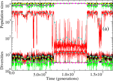
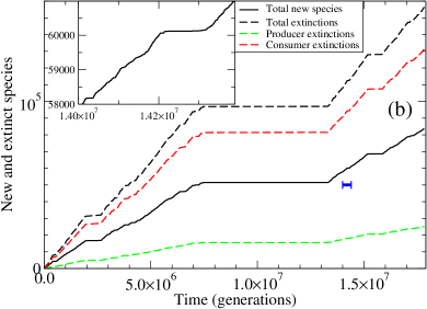
Figure 1: (Color online.) (a) Time series of diversities (measured in species, lower curves) and population sizes (measured in individuals, upper curves) for one specific simulation run. The strongly fluctuating curves in the background are sampled every 8192 generations, while the smooth curves with data points in contrasting colors that are overlaid in the foreground are running averages over 524 288 generations. Black with light gray (yellow online) overlay: all species. Light gray with dark gray overlay (green and magenta online): producers. Dark gray with light gray overlay (red and cyan online): consumers. (b) Time series of the accumulation of new and extinct species in the same simulation run depicted in (a). The solid, black curve shows the total number of different species that have at least once attained a population size $n_{I}>1000$ by time $t$. The dashed curves count the total number of species that have gone extinct after attaining a maximum population greater than 1000. The black dashed curve refers to all species, the light gray one (green online) to producers, and the dark gray one (red online) to consumers. The ratio of approximately 1.89 between the dashed and full black curves indicate that major species recur on average about twice during the evolution. This is an artifact of the finite genome length. The inset shows the detailed, intermittent structure of the solid, black curve over $400\,000$ generations. The interval is indicated by a horizontal bar in the main panel.

Time series of diversities (effective numbers of species) and population sizes for one realization are shown in Fig. 1. To filter out noise from low-population, unsuccessful mutations, we define the diversity as the exponential Shannon-Wiener index.KREB89 This is the exponential function of the information-theoretical entropy of the population distributions, $D(t)=\exp\left[S\left(\{n_{I}(t)\}\right)\right]$, where

$$S\left(\{n_{I}(t)\}\right)=-\sum_{\{I|\rho_{I}(t)>0\}}\rho_{I}(t)\ln\rho_{I}(t)$$ (10)

with $\rho_{I}(t)=n_{I}(t)/N_{\rm tot}(t)$ for the case of all species, and analogously for the producers and consumers separately.

The time series for both diversities and population sizes show intermittent behavior with quiet periods of varying lengths, separated by periods of high evolutionary activity. In this respect, the results are similar to those seen for Models A and B in earlier work.RIKV03 ; RIKV03A ; RIKV05A ; SEVI06 ; RIKV06 However, diverse communities in this model seem to be less stable than those produced by the linear models. In particular, this model has a tendency to flip randomly between an active phase with a diversity near ten, and a “garden of Eden” phase of one or a few producers with a very low population of unstable consumers, such as the one seen around 10 million generations in Fig. 1.

III.2 Power-spectral densities

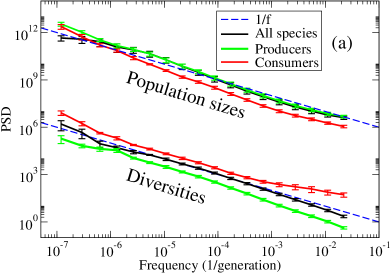
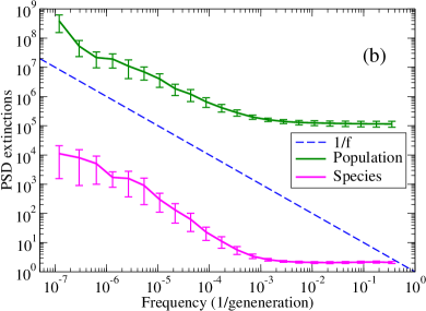
Figure 2: (Color online.) (a) PSDs for the diversities and population sizes, each recorded separately for all species and for producers and consumers. The time series were sampled every 16 generations. (b) PSDs for the extinction activity. In both parts of the figure, the results are averaged over five independent simulation runs. See discussion in the text.

A common method to obtain information about the intensity of fluctuations in a time series at different time scales is the power-spectral density (squared Fourier transform), or PSD. PSDs are presented in Fig. 2 for the diversity fluctuations and the fluctuations in the population sizes (Fig. 2(a)) and the intensity of extinction events (Fig. 2(b)). The former two are shown for the total population, as well as separately for the producers and consumers. All three are similar. Extinction events are recorded as the number of species that have attained a population size greater than one, which go extinct in generation $t$ (marked as “species” in the figure), while extinction sizes are calculated by adding the maximum populations attained by all species that go extinct in generation $t$ (marked as “population” in the figure). The PSDs for all the quantities shown exhibit approximate $1/f$ behavior. For the diversities and population sizes, this power law extends over more than five decades in time. The extinction measures, on the other hand, have a large background of white noise for frequencies above $10^{-3}$ generations^-1, probably due to the high rate of extinction of unsuccessful mutants. For lower frequencies, however, the behavior is consistent with $1/f$ noise within the limited accuracy of our results.

III.3 Species lifetimes and durations of quiet periods

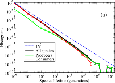
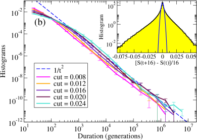
Figure 3: (Color online.) (a) Histograms of species lifetimes, shown for all species, as well as separately for producers and consumers. (b) Histograms of the durations of evolutionarily quiet periods, defined as the times that $|{\rm d}S/{\rm d}t|$ (averaged over 16 generations) falls continuously below some cutoff. The inset is a histogram of ${\rm d}S/{\rm d}t$, showing a Gaussian center with approximately exponential wings. The parabola in the foreground is a Gaussian fit to this central peak. The cutoff values for the main figure, between 0.008 and 0.024, were chosen on the basis of this distribution. The data in both parts of the figure are averaged over five independent simulation runs.

The evolutionary dynamics can also be characterized by histograms of characteristic time intervals, such as the time from creation till extinction of a species (species lifetimes) or the time intervals during which some indicator of evolutionary activity remains continuously below a chosen cutoff (duration of evolutionarily quiet periods). Histograms of species lifetimes are shown in Fig. 3(a). As our indicator of evolutionary activity we use the magnitude of the logarithmic derivative of the diversity, $|{\rm d}S/{\rm d}t|$, and histograms for the resulting durations of quiet periods, calculated with different cutoffs, are shown in Fig. 3(b). Both quantities display approximate power-law behavior with an exponent near $-2$, consistent with the $1/f$ behavior observed in the PSDs.RIKV03 ; PROC83 It is interesting to note that the distributions for these two quantities for this model have approximately the same exponent. This is consistent with the previously studied, mutualistic Model A,RIKV03 ; RIKV05A but not with the predator-prey Model B.RIKV05A ; RIKV06 ; RIKV06B We believe the linking of the power laws for the species lifetimes and the duration of quiet periods indicate that the communities formed by the model are relatively fragile, so that all member species tend to go extinct together in a “mass extinction.” In contrast, Model B produces simple food webs that are much more resilient against the loss of a few species, and as a result the distribution of quiet-period durations decays with an exponent near $-1$.RIKV05A ; RIKV06 ; RIKV06B

IV Adaptive Foraging

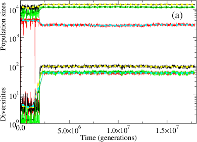
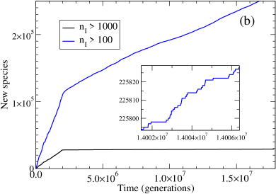
Figure 4: (Color online.) (a) Time series of population sizes (upper curves) and diversities (lower curves) for the model with adaptive foraging. The interpretation of the colors and lines are the same as in Fig. 1(a). (b) Time series of the number of new species that have reached a population greater than 1000 (lower curve) and greater than 100 (upper curve). The inset shows the intermittent structure of the upper curve on a very fine scale of 2000 generations. See discussion in the text.

The model studied above is one in which species forage indiscriminately over all available resources, with the output only limited by competition. Also, there is an implication that an individual’s total foraging effort increases proportionally with the number of species to which it is connected by a positive $M_{IJ}$. A more realistic picture would be that an individual’s total foraging effort is constant and can either be divided equally, or concentrated on richer resources. This is known as adaptive foraging. While one can go to great length devising optimal foraging strategies,DROS01B ; DROS04 we here only use a simple scheme, in which individuals of $I$ show a preference for prey species $J$, based on the interactions and population sizes (uncorrected for interspecific competition) and given by

$$g_{IJ}=\frac{M_{IJ}n_{J}}{\eta_{I}R+\sum_{K}^{{\rm prey}(I)}M_{IK}n_{K}}\;,$$ (11)

and analogously for $R$ by

$$g_{IR}=\frac{\eta_{I}R}{\eta_{I}R+\sum_{K}^{{\rm prey}(I)}M_{IK}n_{K}}\;.$$ (12)

The total foraging effort is thus $g_{IR}+\sum_{J}^{{\rm prey}(I)}g_{IJ}=1$. The preference factors are used to modify the reproduction probabilities by replacing all occurrences of $M_{IJ}$ by $M_{IJ}g_{IJ}$ and of $\eta_{I}$ by $\eta_{I}g_{IR}$ in Eqs. (3–7).

The results of implementing the adaptive foraging are quite striking. The system appears now to have a metastable low-diversity phase similar to the active phase of the non-adaptive model, from which it switches at a random time to an apparently stable high-diversity phase with much smaller fluctuations. As seen in Fig. 4(a), the switchover is quite abrupt, and Fig. 4(b) shows that it is accompanied by a sudden reduction in the rate of creation of new species. As seen in Fig. 5, the PSDs for both the diversities and population sizes in both phases show approximate $1/f$ noise for frequencies above $10^{-5}$ generations^-1. For lower frequencies, the metastable phase shows no discernible frequency dependence, while for the stable phase, the frequency dependence continues at least another decade. It thus appears that long-time correlations are not seen beyond $10^{5}$ generations for the metastable phase, and probably not beyond about $10^{6}$ generations for the stable one. These observations are consistent with species-lifetime distributions for both phases (not shown), which are quite similar to those for the non-adaptive model, but typically with cutoffs in the range of $10^{5}$ to $10^{6}$ generations, much shorter than the total simulation times.

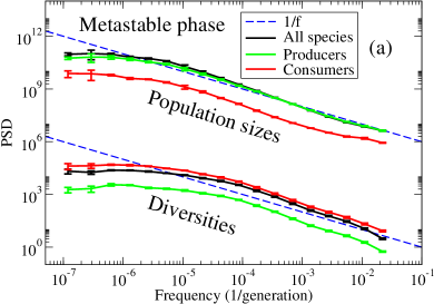
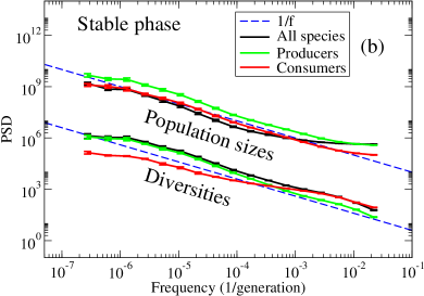
Figure 5: (Color online.) PSDs for the diversities and population sizes in the metastable phase (averaged over three independent runs) (a), and the stable phase (averaged over five independent runs) (b) for the model with adaptive foraging. Both show approximate $1/f$ noise for frequencies above about $10^{-5}$, but the PSDs appear to approach constant levels for the lowest frequencies.

In fact, the system can also escape from the low-diversity phase to total extinction, which is an absorbing state, and in some of our simulation runs we avoided this by limiting $|M_{IJ}|$ to less than 0.9. This restriction does not seem to have any effect on the dynamics in the high-diversity phase. These results are preliminary, and it is possible that the high-diversity phase corresponds to a mutational meltdown. More research is clearly needed regarding the effects of adaptive foraging in this model.

V Conclusions

In this paper we have shown that very complex and diverse dynamical behavior results, even from highly over-simplified models of biological macroevolution. In particular, PSDs that show $1/f$-like noise and power-law lifetime distributions for species as well as evolutionarily quiet states are generally seen. This is the case, both in the analytically tractable, but somewhat unrealistic tangled-nature type models, and in the nonlinear predator-prey models based on the more realistic Holling Type II functional response. Particularly intriguing is the appearance of a new, stable high-diversity phase in the latter type of model when adaptive foraging behavior is included. Among the many questions about this new phase that remain to be addressed is the structure of the resulting community food webs.

References

- (1) B. Drossel, Adv. Phys. 50, 209 (2001).
- (2) M. Hall, K. Christensen, S. A. di Collobiano, and H. J. Jensen, Phys. Rev. E 66, 011904 (2002).
- (3) K. Christensen, S. A. di Collobiano, M. Hall, and H. J. Jensen, J. theor. Biol. 216, 73 (2002).
- (4) S. A. di Collobiano, K. Christensen, and H. J. Jensen, J. Phys. A 36, 883 (2003).
- (5) P. A. Rikvold and R. K. P. Zia, Phys. Rev. E 68, 031913 (2003).
- (6) P. A. Rikvold and R. K. P. Zia, in Computer Simulation Studies in Condensed Matter Physics XVI, edited by D. P. Landau, S. P. Lewis, and H.-B. Schüttler (Springer-Verlag, Berlin, 2004), pp. 34–37.
- (7) R. K. P. Zia and P. A. Rikvold, J. Phys. A 37, 5135 (2004).
- (8) P. A. Rikvold, in Noise in Complex Systems and Stochastic Dynamics III, edited by L. B. Kish, K. Lindenberg, and Z. Gingl (SPIE, The International Society for Optical Engineering, Bellingham, WA, 2005), pp. 148–155, e-print arXiv:q-bio.PE/0502046.
- (9) V. Sevim and P. A. Rikvold, in Computer Simulation Studies in Condensed Matter Physics XVII, edited by D. P. Landau, S. P. Lewis, and H.-B. Schüttler (Springer-Verlag, Berlin, 2005), pp. 90–94.
- (10) V. Sevim and P. A. Rikvold, J. Phys. A 38, 9475 (2005).
- (11) P. A. Rikvold, arXiv:q-bio.PE/0508025.
- (12) M. Eigen, Naturwissenschaften 58, 465 (1971).
- (13) M. Eigen, J. McCaskill, and P. Schuster, J. Phys. Chem. 92, 6881 (1988).
- (14) J. D. Murray, Mathematical Biology (Springer-Verlag, Berlin, 1989).
- (15) P. F. Verhulst, Corres. Math. et Physique 10, 113 (1838).
- (16) R. V. Solé and J. Bascompte, Proc. R. Soc. Lond. B 263, 161 (1996).
- (17) P. A. Rikvold, in preparation.
- (18) B. Drossel, P. G. Higgs, and A. J. McKane, J. theor. Biol. 208, 91 (2001).
- (19) C. J. Krebs, Ecology. The Experimental Analysis of Distribution and Abundance. Fifth Edition. (Benjamin Cummings, San Francisco, 2001).
- (20) G. T. Skalski and J. F. Gilliam, Ecology 82, 3083 (2001).
- (21) Y. Kuang, J. Biomath. 17, 129 (2002).
- (22) B. Drossel, A. McKane, and C. Quince, J. theor. Biol. 229, 539 (2004).
- (23) N. D. Martinez, R. J. Williams, and J. A. Dunne, in Ecological Networks: Linking structure to dynamics in food webs, edited by M. Pasqual and J. A. Dunne (Oxford University Press, Oxford, 2006), pp. 163–185.
- (24) P. A. Abrams, Ecology 75, 1842 (1994).
- (25) H. Resit, R. Arditi, and L. R. Ginzburg, Ecology 76, 995 (1995).
- (26) C. J. Krebs, Ecological Methodology (Harper & Row, New York, 1989), chap. 10.
- (27) I. Procaccia and H. Schuster, Phys. Rev. A 28, 1210 (1983).