Neutral Evolution as Diffusion in phenotype space: reproduction with mutation but without selection

Abstract

The process of ‘Evolutionary Diffusion’, i.e. reproduction with local mutation but without selection in a biological population, resembles standard Diffusion in many ways. However, Evolutionary Diffusion allows the formation of localized peaks that undergo drift, even in the infinite population limit. We relate a microscopic evolution model to a stochastic model which we solve fully. This allows us to understand the large population limit, relates evolution to diffusion, and shows that independent local mutations act as a diffusion of interacting particles taking larger steps.

Reproduction involving random mutations seems at first to lead to a diffusion of the population in type space, however the diffusion involved is anomalous in various ways. A localized configuration that we call a ‘peak’ forms in type space Gavrilets (2004); Forster et al. (2005), and diffuses as a single entity. The variations in the peak width increase as the peak width itself with increasing population size, rendering the infinite population limit meaningless. In contrast, the distribution of a large number of non-interacting particles undergoing local diffusion forms a Normal Distribution with width increasing in time. We will argue that a completely solvable stochastic differential equation model captures the same dynamics as the microscopic evolution process, and provides a meaningful description for the large population limit. We show that although mutations are independent, the effective diffusion is not.

Much previous work on the clustering of individuals in type space focuses on the genealogical lineage. Ref. Derrida and Peliti (1991) provides a comprehensive discussion and a complete solution from this viewpoint. We imagine a population of fixed size $N$, and in each generation, some individuals can expect to have many offspring and others will have none. After some time the whole population will have the same common ancestor, by the process of Gamblers ruinBailey (1964), and hence must have similar type.

Lineage analysis is a good tool to study high dimensional genotype spaces. The theory of Critical Branching ProcessesSlade (2002) finds that in high dimensions ($d>d_{c}$, where the critical dimension $d_{c}=2$ Winter (2002)) describing genotype space, birth/death dynamics are described fully by the lineages. A lineage remains distinct until all individuals in it die. However, in low dimensions ($d\leq d_{c}$) describing phenotypes, additional clustering within a distribution occurs. Although sometimes distinct, the clusters in phenotype space can merge, and hence clusters are poorly defined entities. Instead, a careful average over the distribution that we call a ‘peak’ provides a more useful description. Low dimensional clustering due to birth-death processes was previously only understood in real space Yi-Cheng Zhang et al. (1990); Meyer et al. (1996), with neutral phenotype clustering addressed indirectly Kessler et al. (1997); Ohta and Kimura (1973).

The clustering described above is fluctuation driven. Fluctuations must be considered in evolution unless the number of individuals per type is highTraulsen et al. (2006), or there is strong selection Yi-Cheng Zhang (1997). Otherwise, there is always a region in type space in which the population is small, and therefore there is an area of the equilibrium distribution that is affected by noise. It is (only) in the fluctuations that Evolutionary Diffusion differs from normal Diffusion.

Understanding neutral evolution (i.e. reproduction with mutation but without selection) is of great importance due to its wide usage in numerous contexts, from Genealogical Trees Serva (2004, 2002); Rannala and Yang (1996), to models of mutations in RNA Kimura (1983); Bastolla et al. (2002). Neutral models provide good matches with observed Species-Area Relations and Species-Abundance DistributionsHubbell (2001).

Microscopic model: We are interested in the distribution of types in a population of individuals as they evolve. For comparison to Diffusion, we assume that the total population $N(t)=N$ is constant, a restraint that can easily be relaxed. In addition, we use the simplest type space, namely the 1-dimensional set of integers. However, the qualitative behavior discussed will remain the same in all large connected type spaces. The timestep for the microscopic processes we consider are:

The Diffusion Process:

1. Select an individual $i$ (at position $x$), each with probability $1/N$.

2. Move to $y=x\pm 1$ each with probability $p_{m}/2$, or leave at $y=x$ with probability $1-p_{m}$.

The Evolutionary Diffusion process (which is the Moran process Moran (1962) for a type distribution):

1. Select an individual $i$ (at position $x$), each with probability $1/N$ and mark for killing.

2. Select an individual $j$ (at position $x_{j}$) for reproduction, each with probability $1/N$.

3. Remove individual $i$, and create an offspring of individual $j$ at $y=x_{j}$ with probability $(1-p_{m})$, or mutate to $y=x_{j}\pm 1$ each with probability $p_{m}/2$. Hence the effective diffusive step is $y-x$.

We will refer to properties of the Diffusion process with the subscript $D$, and the Evolutionary Diffusion process with the subscript $E$, e.g. ${\langle x\rangle}_{E}(t)$ for the mean position of the individuals in the evolution process after $t$ timesteps. Time is best measured in generational time $T=t/N$. Care is needed when averaging: we will use the ensemble average (over many realizations) of a quantity $V$ $\overline{V}(t)$, population average $\langle V\rangle(t)=\sum_{i}^{N}V_{i}(t)/N$ and time average up to time $\tau$: $\langle V\rangle=\sum_{t=t_{0}}^{\tau}V(t)/(\tau-t_{0})$. Quantities calculated from probabilities are by definition ensemble averages, and so the notation refers to which average is taken first. See Derrida and Peliti (1991) for further details.

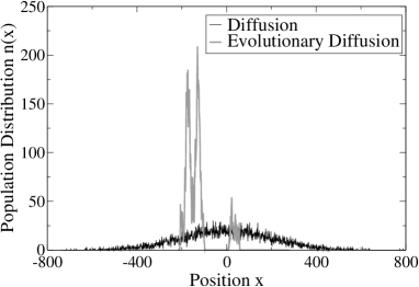
Figure 1: A snapshot of the distribution after $80000$ generations, using $N=10000$ and $p_{m}=0.5$, comparing Evolutionary Diffusion (grey line) and Diffusion (black line). Diffusion follows a (noisy) Normal distribution whereas Evolutionary Diffusion is localized as $2$ clusters, which we combine as a ’peak’ of width $w$ and position $\mu$ undergoing drift.

The number of individuals on site $x$ is $n(x,t)$, and the initial conditions are $n(x=0,t=0)=N$, $n(x,t)=0$ for $x\neq 0$. The ensemble average of the population distribution $\overline{n}(x,t)$ is obtained directly from the Master equation, and is identical for both Diffusion and Evolutionary Diffusion:

$$\frac{\Delta\overline{n}(x,t)}{\Delta t}=\frac{p_{m}}{2N}\bigtriangledown^{2}\overline{n}(x,t).$$ (1)

Hence the (one-point) ensemble average of the two processes is the same, but numerical simulations (Fig. 1) reveals very different behavior. From the figure, we see that Diffusion has followed the ensemble average: a Normal distribution centered on $0$, increasing in width with timePaul and Baschnagel (1999). Although we shall see that the Evolutionary Diffusion process self-averages over time, the thermodynamic limit is subtle. In order to understand why, we now split the peak up into its mean position and standard deviation to create a “Theory of evolutionary peaks”.

Theory of evolutionary peaks: We define here conceptually simple and solvable processes of Evolutionary Diffusion and Diffusion which we argue captures the essential features of the microscopic models. The distribution is described as a ‘peak’: a Normal distribution with mean $\mu(t)$ and standard deviation (i.e. width) $w(t)$, which vary as a product of the dynamics. The probability distribution is continuous, but a discrete ‘individual’ of size $1/N$ is moved per timestep. Although a given realization of a peak never resembles a Normal distribution, this is a good model of the evolutionary process because a Normal distribution is a good approximation for the time average of the peaks in the variable $x^{\prime}=x-\mu(t)$ (we now drop the dash notation); see Fig. 2. We hence ‘integrate out’ the inessential degrees of freedom: the particular distribution of individuals within the peak.

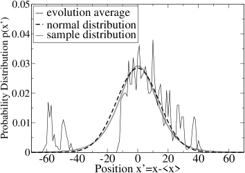
Figure 2: Time-averaged Evolutionary Diffusion distribution (solid line), Normal distribution (dashed line) with standard deviation calculated from theory in Eq. (17). The two agree up to the second moment. Also shown is a snapshot of the distribution (thin line). ($N=1000$, $p_{m}=0.5$)

In the evolutionary process, in each timestep a death will occur at any point $x$ in the distribution $p(x)$:

$$p_{E}(x;\mu=0,w)=\frac{e^{-x^{2}/2w^{2}}}{\sqrt{2\pi}w}.$$ (2)

The parent position $x_{j}$ will be drawn independently from the same distribution, and the offspring will be mutated with probability $p_{m}$ to $y\pm 1$. Hence the distribution for births $p(y)$ is:

$$p_{E}(y;\mu=0,w) =(1-p_{m})\frac{e^{-y^{2}/2w^{2}}}{\sqrt{2\pi}w}$$ (3)

$$+\frac{p_{m}}{2}\Big{[}\frac{e^{-(y-1)^{2}/2w^{2}}}{\sqrt{2\pi}w}+\frac{e^{-(y+1)^{2}/2w^{2}}}{\sqrt{2\pi}w}\Big{]}.$$

The probability distribution for the Diffusion process, moving a particle at $x$ to $x\pm 1$ with probability $p_{m}$, is written as:

$$p_{D}(x;\mu=0,w)= \frac{e^{-x^{2}/2w^{2}}}{\sqrt{2\pi}w},$$ (4)

$$p_{D}(y;\mu=0,w)= (1-p_{m})\delta(y-x)$$ (5)

$$+\frac{p_{m}}{2}[\delta(y-x+1)+\delta(y-x-1)].$$

The expectation value of a variable $V(x,y)$ is simply the integral of $V$ over the probability distribution:

$$\langle V(x,y)\rangle=\int_{-\infty}^{\infty}\int_{-\infty}^{\infty}V(x,y)p(x)p(y)dydx.$$ (6)

Eq. (6) is simple to calculate because all of our probabilities are independently Normal distributed, or interact trivially via delta functions.

We now perform calculations for the expectation values of $w(t+1)$ given $w(t)$, (working with the variance $w^{2}$ for simplicity). We consider the death of individual $q$ at $x_{q}$, which is replaced by a birth occurring at $y_{q}$.

$$w^{2}(t) =\frac{1}{N}\sum_{i=1}^{N}x_{i}^{2}-\left(\sum_{i=1}^{N}\frac{x_{i}}{N}\right)^{2},$$ (7)

$$w^{2}(t+1) =\frac{1}{N}\sum_{i=1}^{N}x_{i}^{2}+\frac{y_{q}^{2}-x_{q}^{2}}{N}-\left(\sum_{i=1}^{N}\frac{x_{i}}{N}+\frac{y_{q}-x_{q}}{N}\right)^{2},$$ (8)

$$F =\Delta w^{2}(t)=w^{2}(t+1)-w^{2}(t)$$

$$=\frac{y_{q}^{2}-x_{q}^{2}}{N}-\frac{y_{q}^{2}+x_{q}^{2}-2x_{q}y_{q}}{N^{2}}.$$ (9)

Here we have defined $F=\Delta w^{2}(t)$ for later use, and used $\sum_{i=1}^{N}x_{i}=0$. These quantities are population averages; we now ensemble average over the possible births and deaths by simple integration over Eq. (6). We find that for the Diffusion process, the expected change in the variance is always positive and independent of $w$:

$$\frac{\Delta\langle w_{D}^{2}(x,y)\rangle}{\Delta t}=\frac{p_{m}}{N}(1-\frac{1}{N}).$$ (10)

For the evolution process, the expected change in the variance is:

$$\frac{\Delta\langle w_{E}^{2}(x,y)\rangle}{\Delta t}=\frac{1}{N}(p^{*}-\frac{2w_{E}^{2}}{N}),$$ (11)

where for brevity we have defined $p^{*}=p_{m}-1/N$ (assumed positive). This time, the rate of change of the variance depends on itself, and there is an equilibrium for which $E(\Delta w_{E}^{2}(x,y))=0$, at $w_{E}^{equil}=\sqrt{{Np^{*}}/{2}}.$ The product $Np^{*}$ is the average number of mutants per generation, minus one. By taking the limit $\Delta t\to 0$ in Eq. (11), and solving by separation of variables, we obtain the variance $\langle w_{E}^{2}\rangle(T)={\frac{Np^{*}}{2}}(1-e^{-2T/N})$.

We now look at how the peak width $w$ varies in time, by considering the fluctuations in $F=\Delta_{t}w^{2}$, the change of peak size. We are interested in fluctuations around the equilibrium standard deviation $w^{equil}$. $w^{equil}$ is not the mean observed value of $w$ - we will be able to correct it by considering higher moments. We will now assume a large population $N\gg 1$, and consider the reduced variable $s=\frac{w}{\sqrt{N}}$ to identify leading order terms.

$$\overline{F^{2}}-\overline{F}^{2} =4s^{4}+{4p_{m}s^{2}}/{N}+\cdots$$

$$\approx\frac{4w^{4}}{N^{2}}.$$ (12)

To represent the particular history of the evolution process we must write Eq. (11) with an additional noise term $\sqrt{\overline{F^{2}}-\overline{F}^{2}}\eta(t)\approx(2w^{2}/N)\eta(t)$, where $\eta(t)$ has mean zero and standard deviation $1$ (keeping up to second order moments in the noise - higher moments are $O(1/N)$ smaller). In generational time $T=t/N$, as $\Delta T\to 0$ we obtain:

$$dw_{E}^{2}(T)\approx\left[p^{*}-\frac{2w^{2}}{N}\right]dT+\frac{2w^{2}}{\sqrt{N}}dW.$$ (13)

Where $W(t)$ is a Wiener processPaul and Baschnagel (1999). We solve by finding the Fokker-Planck equation Kannan (1979):

$$\frac{\partial p(w^{2},T)}{\partial T}+\frac{\partial([p^{*}-2w^{2}/N]p(w^{2},T))}{\partial(w^{2})}$$

$$-\frac{1}{2}\frac{\partial^{2}(4w^{4}p(w^{2},T)/N)}{\partial(w^{2})^{2}}=0.$$ (14)

Seeking the steady state solution $\frac{\partial p(w^{2},T)}{\partial T}=0$, integration twice shows that (for this to be a probability distribution) the unique solution is:

$$p(w^{2})d(w^{2})=\left(\frac{Np^{*}}{2}\right)^{2}\frac{1}{(w^{2})^{3}}e^{-\frac{Np^{*}}{2w^{2}}}d(w^{2}),$$ (15)

$$\implies\,p(w)dw=\frac{(Np^{*})^{2}}{2}\frac{1}{w^{5}}e^{-\frac{Np^{*}}{2w^{2}}}dw.$$ (16)

The tail of $p(w)$ is a power law, corresponding to the existence of multiple (arbitrarily distant) clusters within the peak. From this we can calculate the arithmetic mean of the peak width, corrected for noise:

$$\langle w\rangle=\int_{0}^{\infty}wp(w)dw=\sqrt{\frac{Np^{*}}{2}}\frac{\sqrt{\pi}}{2},$$ (17)

This contrasts with Diffusion, as $\langle w_{D}\rangle$ has no stationary distribution and follows Eq. (10). The standard deviation of the peak width is:

$$\sigma_{w}=\sqrt{\langle w^{2}\rangle-\langle w\rangle^{2}}=\sqrt{{Np^{*}(1-\pi/4)}/{2}}.$$ (18)

Therefore the standard deviation in the peak width increases at the same rate (with N) as the peak width itself. The 4th and higher moments of the distribution of peak widths diverge due to the power law tail of $p(w)$. The model approximations are confirmed by numerics. Both Eq. (13) and $w(t)$ for the ‘Evolutionary Diffusion Process’ defined initially have indistinguishable signals and Power Spectra (not shown), and conform to Eq. (17) to within $2\%$: for $N=10000$ and $p_{m}=1$, with $200$ runs of $10^{5}$ generations, counting $w(t)$ after time $5\times 10^{4}$, we find $\langle w\rangle=64.34\pm 2.14$ for the Evolutionary Diffusion Process, $\langle w\rangle=63.17\pm 1.20$ for Eq. (13), comparing with a theoretical prediction of $\langle w\rangle=62.66$. Eq. (13) is fast to simulate for long times and, as indicated, behaves very similarly to the microscopic process.

We now examine the behavior of the expected root-mean-square (RMS) displacement of the peak center as a function of time; direct integration of $\langle(\Delta x)^{2}\rangle=\langle(x_{q}-y_{q})^{2}/N^{2}\rangle$, using the steady state value $\langle w^{2}_{E}\rangle=Np^{*}/2$ in Eq. (LABEL:eqn:xevsoln), yields the following step size for evolution:

$$\Delta\langle{x\rangle}_{E}^{RMS}(t)\approx\sqrt{{p^{*}}/{N}}.$$ (19)

From random walk theoryPaul and Baschnagel (1999), the mean (RMS) position of a random walker taking steps of size $S$ after $t$ timesteps is $\langle x\rangle^{RMS}=S\sqrt{t}$. Hence:

$${\langle x\rangle}^{RMS}_{D}(T)={\sqrt{p_{m}t}}/{N}=\sqrt{{p_{m}T}/{N}},$$ (20)

$${\langle x\rangle}^{RMS}_{E}(T)=\sqrt{{p^{*}t}/{N}}=\sqrt{p^{*}T}.$$ (21)

Hence, in the limit of infinite $N$ the Diffusion process remains stationary, but in generational time the mean position of the Evolutionary Diffusion process does a random walk of step size independent of the total number of individuals.

For completeness we could write an equation for $\mu(T)={\langle x\rangle}$ for evolution as: $d\mu_{E}(T)=N^{-1/2}\sqrt{p_{m}+2w_{E}^{2}(t)}dW$. This equation together with Eq. 13 describe the system fully and are completely solved once the peak width reaches equilibrium probability distribution.

We have described the microscopic behavior of the evolution of reproducing individuals in a type space, and approximated it to two coupled solvable stochastic processes for the distribution. We find two main differences between Evolutionary Diffusion and normal Diffusion. 1) The short range mutation process effectively becomes a longer ranged (by O($\sqrt{N}$)) diffusive step. By the Central Limit Theorem, the standard deviation of the mean position $\mu$ taking $N$ steps per generation of size $A$ increases as $A\sqrt{N}$. In diffusion, the steps are of size $A=1/N$, but in evolution the steps are of size $A=1/\sqrt{N}$ so the convergence is not fast enough to set the location of the peak center in the infinite population limit. 2) The effective diffusion is not independent and peaks can form with fluctuating width $w$ around $\langle w\rangle$, following the distribution in Eq. (16) which has a power law tail. This provides a null hypothesis to determine if two asexual individuals belonging to different clusters of a phenotype in fact are subject to the same selection pressure, i.e. members of a single neutrally evolving population or ’peak’, or whether differential selection is responsible for the population breaking up into separate clusters. In the neutral case all but one cluster will go extinct. However, if differential selection acts then several clusters of phenotype may survive in separate ‘niches’.

In terms of replicator dynamics, our results transparently explain how a ‘species’ in type space (the peak described above) is able to maintain its coherence as it performs a random walk due to mutation prone reproduction. We found that the distribution of a phenotype in neutral evolution is ‘non-trivial’ regardless of population size. In terms of diffusion, we describe an interesting type of particle interaction that allows for clustering.

DL is funded by an EPSRC studentship, and is grateful to Nelson Bernardino for useful discussions.

References

- Gavrilets (2004) S. Gavrilets, Fitness Landscapes and the Origin of Species (Princeton University Press, 41 William Street, Princeton, New Jersey 08540, 2004).
- Forster et al. (2005) R. Forster, C. Adami, and C. O. Wilke (2005), available from http://arxiv.org/abs/q-bio/0509002.
- Derrida and Peliti (1991) B. Derrida and L. Peliti, Bul. Math. Biol. 53, 355 (1991).
- Bailey (1964) N. T. J. Bailey, The elements of Stochastic Processes (John Wiley and Sons, Inc, New York, 1964).
- Slade (2002) G. Slade, Notices of the AMS 49, 1056 (2002).
- Winter (2002) A. Winter, Elec. J. of Prob. 7, 1 (2002).
- Yi-Cheng Zhang et al. (1990) Yi-Cheng Zhang, Maurizio Serva, and Mikhail Polikarpov, J. Stat. Phys. 58, 849 (1990).
- Meyer et al. (1996) M. Meyer, S. Havlin, and A. Bunde, Phys. Rev. E 54, 5567 (1996).
- Kessler et al. (1997) D. A. Kessler, H. Levine, D. Ridgway, and L. Tsimring, J. Stat. Phys. 87, 519 (1997).
- Ohta and Kimura (1973) T. Ohta and M. Kimura, Genetical Research 22, 201 (1973).
- Traulsen et al. (2006) A. Traulsen, J. C. Claussen, and C. Hauert, Phys. Rev. E 74, 011901 (2006).
- Yi-Cheng Zhang (1997) Yi-Cheng Zhang, Phys. Rev. E 55, R3817 (1997).
- Serva (2004) M. Serva, Physica A 332, 387 (2004).
- Serva (2002) M. Serva (2002), available from http://arxiv.org/abs/cond-mat/0208144.
- Rannala and Yang (1996) B. Rannala and Z. Yang, J. Molec. Evol. 43, 304 (1996).
- Kimura (1983) M. Kimura, The neutral theory of molecular evolution (Cambridge University Press, The Pitt Building, Trumpington Street, Cambridge CB2 1RP, 1983).
- Bastolla et al. (2002) U. Bastolla, M. Porto, H. E. Roman, and M. Vendruscolo, Phys. Rev. Let. 89, 208101 (2002).
- Hubbell (2001) S. Hubbell, The Unified Neutral Theory of Biodiversity and Biogeography (Princeton University Press, 41 William Street, Princeton, New Jersey 08540, 2001).
- Moran (1962) P. A. P. Moran, The Statistical Processes of Evolutionary Theory (Clarendon Press, Oxford, 1962).
- Paul and Baschnagel (1999) W. Paul and J. Baschnagel, Stochastic Processes From Physics to Finance (Springer, 1999).
- Kannan (1979) D. Kannan, An Introduction To Stochastic Processes (Elsevier North Holland, Inc., 52 Vanderbilt Avenue, New York, 10017, 1979).