INSTITUT NATIONAL DE RECHERCHE EN INFORMATIQUE ET EN AUTOMATIQUE

Lagrangian Approaches for a class of Matching Problems in Computational Biology
Nicola Yanev and Rumen Andonov and Philippe Veber and Stefan Balev N° ????
31st August 2006

Abstract: This paper presents efficient algorithms for solving the problem of aligning a protein structure template to a query amino-acid sequence, known as protein threading problem. We consider the problem as a special case of graph matching problem. We give formal graph and integer programming models of the problem. After studying the properties of these models, we propose two kinds of Lagrangian relaxation for solving them. We present experimental results on real life instances showing the efficiency of our approaches.

Key-words: sequence-structure alignment, complexity, integer programming, Lagrangian relaxation

Approches de relaxation lagrangienne pour la résolution d’une classe de problème d’appariement en bioinformatique

Résumé : Cet article propose des algorithmes efficaces pour déterminer l’alignement optimal entre une structure et une séquence protéique, problème connu sous le nom de protein threading. Nous posons ce problème comme un cas particulier d’appariement. Nous présentons un modèle formel du problème sous la forme d’une famille de graphes, et des programmes en nombre entiers correspondants. Nous étudions dans un premier temps les propriétés de ces modèles, pour ensuite proposer deux approches de relaxation lagrangienne pour la résolution. Enfin, nous montrons, à l’aide de données expérimentales sur des instances réelles, l’efficacité de ces approches.

Mots-clés : alignement séquence-structure, complexité, programmation en nombres entiers, relaxation lagrangienne

1 Preliminaries

Matching is important class of combinatorial optimization problems with many real-life applications. Matching problems involve choosing a subset of edges of a graph subject to degree constraints on the vertices. Many alignment problems arising in computational biology are special cases of matching in bipartite graphs. In these problems the vertices of the graph can be nucleotides of a DNA sequence, aminoacids of a protein sequence or secondary structure elements of a protein structure. Unlike classical matching problems, alignment problems have intrinsic order on the graph vertices and this implies extra constraints on the edges. As an example, Fig. 1 shows an alignment of two sequences as a matching in bipartite graph. We can see that the feasible alignments are 1-matchings without crossing edges.

Figure 1: Matching interpretation of sequence alignment problem

In this paper we deal with the problem of aligning a protein structure template to a query protein sequence of length $N$, known as protein threading problem (PTP). A template is an ordered set of $m$ secondary structure elements (or blocks) of lengths $l_{i}$, $i=1,\dots,m$. An alignment (or threading) is covering of contiguous sequence areas by the blocks. A threading is called feasible if the blocks preserve their order and do not overlap. A threading is completely determined by the starting positions of all blocks. For the sake of simplicity we will use relative positions. If block $i$ starts at the $j$th query character, its relative position is $r_{i}=j-\sum_{k=1}^{i-1}l_{k}$. In this way the possible (relative) positions of each segment are between 1 and $n=N+1-\sum_{i=1}^{m}l_{i}$ (see Fig. 2(b)). The set of feasible threadings is

$$\mathcal{T}=\{(r_{1},\dots,r_{m})\;|\;1\leq r_{1}\leq\dots\leq r_{m}\leq n\}.$$

(a)

abs. position	1	2	3	4	5	6	7	8	9	10	11	12	13	14	15	16	17	18	19	20
rel. position block 1	1	2	3	4	5	6	7	8	9
rel. position block 2				1	2	3	4	5	6	7	8	9
rel. position block 3									1	2	3	4	5	6	7	8	9

(b)

(c)

Figure 2: (a) Example of alignment of query sequence of length 20 and template containing 3 segments of lengths 3, 5 and 4. (b) Correspondence between absolute and relative block positions. (c) A matching corresponding to the alignment of (a).

Protein threading problem is a matching problem in a bipartite graph $(U\cup V,U\times V)$, where $U=\{u_{1},\dots,u_{m}\}$ is the ordered set of blocks and $V=\{v_{1},\dots,v_{n}\}$ is the ordered set of relative positions. The threading feasibility conditions can be restated in terms of matching in the following way. A matching $M\subseteq U\times V$ is feasible if:

1. $d(u)=1$, $u\in U$ (where $d(x)$ is the degree of $x$). This means that each block is assigned to exactly one position). By the way this implies that the cardinality of each feasible matching is $m$.

2. There are no crossing edges, or more precisely, if $(u_{i},v_{j})\in M$, $(u_{k},v_{l})\in M$ and $i<k$, then $j\leq l$. This means that the blocks preserve their order and do not overlap. The last inequality is not strict because of using relative positions.

Note that while (i) is a classical matching constraint, (ii) is specific for the alignment problems and makes them more difficult. Fig. 2(c) shows a matching corresponding to a feasible threading.

Proposition 1.

The number of feasible threadings is $|\mathcal{T}|=\tbinom{m+n-1}{m}$.

Proof.

We can define the relative positions as $r_{i}=j-\sum_{k=1}^{i-1}l_{k}+i-1$. In this case the relative positions of the feasible threadings are related by

$$1\leq r_{1}<\dots<r_{m}\leq m+n-1$$

and a threading is determined by choosing $m$ out of $m+n-1$ positions. ∎

One of the possible ways to deal with alignment problems is to try to adapt the existing matching techniques to the new edge constraints of type (ii). Instead of doing this we propose a new graph model and we develop efficient matching algorithms based on this model.

We introduce an alignment graph $G=(U\times V,E)$. Each vertex of this graph corresponds to an edge of the matching graph. For simplicity we will denote the vertices by $v_{ij}$, $i=1,\dots,m$, $j=1,\dots,n$ and draw them as an $n\times m$ grid (see Fig. 3). The vertices $v_{ij}$, $j=1,\dots,n$ will be called $i$th layer. A layer corresponds to a block and each vertex in a layer corresponds to positioning of this block in the query sequence.

One can connect by edges the pairs of vertices of $G$ which correspond to pairs of noncrossing edges in the matching graph. In this case a feasible threading is an $m$-clique in $G$. A similar approach is used in [12]. We introduce only a subset of the above edges, namely the ones that connect vertices from adjacent columns and have the following regular pattern: $E=\{(v_{ij},v_{i+1,l})\;|\;i=1,\dots,m-1,1\leq j\leq l\leq n\}$. We add two more vertices $S$ and $T$ and edges connecting $S$ to all vertices from the first column and $T$ to all vertices from the last column. Now it is easy to see the one-to-one correspondence between the set of feasible threadings (or matchings) and the set of $S$-$T$ paths in $G$. Fig. 3 illustrates this correspondence.

Figure 3: Example of alignment graph. The path in thick lines corresponds to the threading in which the positions of the blocks are 1,2,2,3,4,4.

Till now we gave several alternative ways to describe the feasible alignments. Alignment problems in computational biology involve choosing the best of them based on some score function. The simplest score functions associate weights to the edges of the matching graph. For example, this is the case of sequence alignment problems. By introducing alignment graphs similar to the above, classical sequence alignment algorithms, such as Smith-Waterman or Needleman-Wunch, can be viewed as finding shortest $S$-$T$ paths. When the score functions use structural information, the problems are more difficult and the shortest path model cannot incorporate this information.

The score functions in PTP evaluate the degree of compatibility between the sequence amino acids and their positions in the template blocks. The interactions (or links) between the template blocks are described by the so-called generalized contact map graph, whose vertices are the blocks and whose edges connect pairs of interacting blocks. Let $L$ be the set of these edges:

$$L=\{(i,k)\;|\;i<k\text{ and blocks $i$ and $k$ interact}\}$$

Sometimes we need to distinguish the links between adjacent blocks and the other links. Let $R=\{(i,k)\;|\;(i,k)\in L,\;k-i>1\}$ be the set of remote (or non-local) links. The links from $L\setminus R$ are called local links. Without loss of generality we can suppose that all pairs of adjacent blocks interact.

The links between the blocks generate scores which depend on the block positions. In this way a score function of PTP can be presented by the following sets of coefficients

• $c_{ij}$, $i=1,\dots,m$, $j=1,\dots,n$, the score of putting block $i$ on position $j$

• $d_{ijkl}$, $(i,k)\in L$, $1\leq j\leq l\leq n$, the score generated by the interaction between blocks $i$ and $k$ when block $i$ is on position $j$ and block $k$ is on position $l$.

The coefficients $c_{ij}$ are some function (usually sum) of the preferences of each query amino acid placed in block $i$ for occupying its assigned position, as well as the scores of pairwise interactions between amino acids belonging to block $i$. The coefficients $d_{ijkl}$ include the scores of interactions between pairs of amino acids belonging to blocks $i$ and $j$. Loops (sequences between adjacent blocks) may also have sequence specific scores, included in the coefficients $d_{i,j,i+1,l}$.

The score of a threading is the sum of the corresponding score coefficients and PTP is the optimization problem of finding the threading of minimum score. If there are no remote links (if $R=\emptyset$) we can put the score coefficients on the vertices and the edges of the alignment graph and PTP is equivalent to the problem of finding the shortest $S$-$T$ path. In order to take the remote links into account, we add to the alignment graph the edges

$$\{(v_{ij},v_{kl})\;|\;(i,k)\in R,\;1\leq j\leq l\leq n\}$$

which we will refer as $z$-edges.

An $S$-$T$ path is said to activate the $z$-edges that have both ends on this path. Each $S$-$T$ path activates exactly $|R|$ $z$-edges, one for each link in $R$. The subgraph induced by the edges of an $S$-$T$ path and the activated $z$-edges is called augmented path. Thus PTP is equivalent to finding the shortest augmented path in the alignment graph (see Fig. 4).

Figure 4: Example of augmented path. The generalized contact map graph is given in the bottom. The $x$ arcs of the $S$-$T$ path are in solid lines. The activated $z$-arcs are in dashed lines. The length of the augmented path is equal to the score of the threading $(1,2,2,3,4,4)$.

As we will see later, the main advantage of this graph is that some simple alignment problems reduce to finding the shortest $S$-$T$ path in it with some prices associated to the edges and/or vertices. The last problem can be easily solved by a trivial dynamic programming algorithm of complexity $O(mn^{2})$. In order to address the general case we need to represent this graph optimisation problem as an integer programming problem.

2 Integer programming formulation

Let $y_{ij}$ be binary variables associated to the vertices of $G$. $y_{ij}$ is one if block $i$ is on position $j$ and zero otherwise. Let $Y$ be the polytope defined by the following constraints:

$$\sum_{j=1}^{n}y_{ij}=1 i=1,\dots,m$$ (1)

$$\sum_{l=1}^{j}y_{il}-\sum_{l=1}^{j}y_{i+1,l}\geq 0 i=1,\dots,m-1,\;j=1,\dots,n-1$$ (2)

$$y_{ij}\geq 0 i=1,\dots,m,\;j=1,\dots,n$$ (3)

Constraints (1) ensure the feasibility condition (i) and (2) are responsible for (ii). That is why $Y\cap B^{mn}$ is exactly the set of feasible threadings.

In order to take into account the interaction costs, we introduce a second set of binary variables $z_{ijkl}$, $(i,k)\in L$, $1\leq j\leq l\leq n$. To avoid added notation we will use vector notation for the variables $y_{i}=(y_{i1},...y_{in})\in B^{n}$ with assigned costs $c_{i}=(c_{i1},...c_{in})\in R^{n}$ and $z_{ik}=(z_{i1k1},\ldots,z_{i1kn},z_{i2k2},\ldots,z_{i2kn},\ldots,z_{inkn})\in B^{\frac{n(n+1)}{2}}$ for $(i,k)\in L$ with assigned costs $d_{ik}=(d_{i1k1},\ldots,d_{i1kn},d_{i2k2},\ldots,d_{i2kn},\ldots,d_{inkn})\in R^{\frac{n(n+1)}{2}}$.

Consider the $2n\times\frac{n(n+1)}{2}$ node-edge incidence matrix of the subgraph spanned by two interacting layers $i$ and $k$. The submatrix $A^{\prime}$ containing the first $n$ rows (resp. $A^{\prime\prime}$ containg the last $n$ rows) corresponds to the layer $i$ (resp. layer $k$).

Now the protein threading problem can be defined as

$$z_{IP}^{L}=v(PTP(L))=\min\{\sum_{i=1}^{m}c_{i}y_{i}+\sum_{(i,k)\in L}d_{ik}z_{ik}\}$$ (4)

subject to: $$y=(y_{1},\dots,y_{m})\in Y,$$ (5)

$$y_{i}=A^{\prime}z_{ik} (i,k)\in L$$ (6)

$$y_{k}=A^{\prime\prime}z_{ik} (i,k)\in L$$ (7)

$$z_{ik}\in B^{\frac{n(n+1)}{2}} (i,k)\in L$$ (8)

The shortcut notation $v(.)$ will be used for the optimal objective function value of a subproblem obtained from $PTP(L)$ with some $z$ variables fixed.

3 Complexity results

In this section we study the structure of the polytope defined by (5)-(7) and $z_{ik}\in R_{+}^{\frac{n(n+1)}{2}}$, as well as the impact of the set $L$ on the complexity of the algorithms for solving the $PTP$ problem. Throughout this section, vertex costs $c_{i}$ are assumed to be zero. This assumption is not restrictive because the costs $c_{ij}$ can be added to $d_{i,j,i+1,l}$, $l=j,\dots,n$. We will consider the costs $d_{ik}$ as $n\times n$ matrices containing the coefficients $d_{ijkl}$ above the main diagonal and arbitrary large numbers below the main diagonal. In order to simplify the descriptions of the algorithms given in this section we introduce the following matrix operations.

Definition 1.

Let $A$ and $B$ be two matrices of compatible size. $A\cdot B$ is the matrix product of $A$ and $B$ where the addition operation is replaced by “$\min$” and the multiplication operation is replaced by “+”.

Definition 2.

Let $A$ and $B$ be two matrices of size $n\times n$. $M=A\otimes B$ is defined by $M(i,j)=\min_{i\leq r\leq j}A(i,r)+B(i,j)$

Below we present four kinds of contact graphs that make PTP polynomially solvable.

3.1 Contact graph contains only local edges

As mentioned above, in this case PTP reduces to finding the shortest $S$-$T$ path in the alignment graph which can be done by $O(mn^{2})$ dynamic programming algorithm. An important property of an alignment graph containing only local edges is that it has a tight LP description.

Theorem 1.

The polytope $Y$ is integral, i.e. it has only integer-valued vertices.

Proof.

Let $A$ be the matrix of the coefficients in (1)-(2) with columns numbered by the indices of the variables. One can prove that $A$ is totaly unimodular (TU) by performing the following sequence of TU preserving transformations.

for $i=1,\dots,n$
       delete column $(i,n)$ (these are unit columns)
    for $i=1,\dots,m$
       for $j=n-1,\dots,1$
          pivot on $a_{ij}$ ($A$ is TU iff the matrix obtained by a pivot operation on $A$ is TU
          delete column $(i,j)$ (now this is unit column)

The final matrix is an unit column that is TU. Since all the transformations are TU preserving, $A$ is TU and $Y$ is integral.

One could prove the same assertion by showing that an arbitrary feasible solution to (1)-(3) is a convex combination of some integer-valued vertices of $Y$. The best such vertex (in the sense of an objective function) might be a good approximate solution to a problem whose feasible set is an intersection of $Y$ with additional constraints.

Let $y$ is an arbitrary non -integer solution to (1)-(3). Because of (1), (2) an unit flow $f=(f_{sj},\;f_{(i,k)(i+1,j)})\;\;i=1,m-1\;\;j=1,n\;\;$ in $G$ exist s.t.

$$\sum_{k\leq j}f_{(i,k)(i+1,j)}=y_{ij}\;\;i=1,m-1\;\;f_{sj}=y_{1j}\;\;j=1,n$$

By the well known properties of the network flow polytope, the flow $f$ can be expressed as a convex combination of integer-valued unit flows (paths in $G)$. But each such flow corresponds to an integer-valued $y$, i.e. $y_{ij}=f_{(i-1,k)(ij)}=1$. Thus, the convex combination of the paths that gives $f$ is equivalent to a convex combination of the respective vertices of $Y$ that gives $y$.

The details for efficiently finding of the set of the vertices participating in the convex combination could be easily stressed by this sketch of the prove. ∎

3.2 Contact graph contains no crossing edges

Two links $(i_{1},k_{1})$ and $(i_{2},k_{2})$ such that $i_{1}<i_{2}$ are said to be crossing when $k_{1}$ is in the open interval $(i_{2},k_{2})$. The case when the contact graph $L$ contains no crossing edges has been mentioned to be polynomially solvable for the first time in [1]. Here we present a different sketch for $O(mn^{3})$ complexity of PTP in this case.

If $L$ contains no crossing edges, then $PTP(L)$ can be recursively divided into independent subproblems. Each of them consists in computing all shortest paths between the vertices of two layers $i$ and $k$, discarding links that are not included in $(i,k)$. The result of this computation is a distance matrix $D_{ik}$ such that $D_{ik}(j,l)$ is the optimal length between vertices $(i,j)$ and $(k,l)$. Note that for $j>l$, as there is no path in the graph, $D_{ik}(j,l)$ is an arbitrarily large coefficient. Finally, the solution of $PTP(L)$ is the smallest entry of $D_{1m}$.

We say that a link $(i,k),i<k$ is included in the interval $[a,b]$ when $[i,k]\subseteq[a,b]$. Let us denote by $L_{(ik)}$ the set of links of $L$ included in $[i,k]$. Then, an algorithm to compute $D_{ik}$ can be sketched as follows:

1. If $L_{(ik)}=\{(i,k)\}$ then the distance matrix is given by

   $$D_{ik}=\left\{\begin{array}[]{ll}d_{ik}&\mbox{if}(i,k)\in L\\ \tilde{0}&\mbox{otherwise}\end{array}\right.$$ (9)

   where $\tilde{0}$ is an upper triangular matrix in the previously defined sense (arbitrary large coefficients below the main diagonal) and having only zeros in its upper part.

2. Otherwise, as $L_{(ik)}$ has no crossing edges, there exists some $s\in[i,k]$ such that any edge of $L_{(ik)}$ except $(i,k)$ is included either in $[i,s]$ or in $[s,k]$. Then

   $$D_{ik}=\left\{\begin{array}[]{ll}D_{is}\cdot D_{sk}+d_{ik}&\mbox{if}(i,k)\in L\\ D_{is}\cdot D_{sk}&\mbox{otherwise}\end{array}\right.$$ (10)

If the contact graph has $m$ vertices, and contains no crossing edges, then the problem is decomposed into $O(m)$ subproblems. For each of them, the computation of the corresponding distance matrix is a $O(n^{3})$ procedure (matrix multiplication with $(\min,+)$ operations). Overall complexity is thus $O(mn^{3})$. Typically, $n$ is one or two orders of magnitude greater than $m$, and in practice, this special case is already expensive to solve.

3.3 Contact graph is a single star

A set of edges $L_{(i)}=\{(i,k_{1}),\dots,(i,k_{r})\}$, $k_{1}<k_{2}<\ldots k_{r}$ is called a star.

Theorem 2.

Let $L_{(i)}=\{(i,k_{1}),\dots,(i,k_{r})\}$ be a star. Then $D_{ik_{r}}=(\dots(d_{ik_{1}}\otimes d_{ik_{2}})\otimes\dots)\otimes d_{ik_{r}}$.

Proof.

The proof follows the basic dynamic programming recursion for this particular case: for the star $L=\{(i,k_{1}),\dots,(i,k_{r})\}=L^{\prime}\bigcup\{(i,k_{r})\}$, we have $v(L:z_{ijk_{r}l}=1)=d_{ijk_{r}l}+\min_{j\leq s\leq l}v(L^{\prime}:z_{ijk_{r-1}s}=1)$. ∎

In order to compute $A\otimes B$, we use the following recursion: let $M^{\prime}$ be the matrix defined by $M^{\prime}(i,j)=\min_{i\leq r\leq j}A(i,r)$, then

$$M^{\prime}(i,j)=\min\{M^{\prime}(i,j-1),A(i,j)\},\mbox{ for all }j\geq i$$

Finally $A\otimes B=M^{\prime}+B$. From this it is clear that $\otimes$ multiplication for $n\times n$ matrices is of complexity $O(n^{2})$ and hence the complexity of PTP in this case is $O(rn^{2})$.

3.4 Contact graph is decomposable

Given a contact graph $L=\{(i_{1},k_{1}),\dots,(i_{r},k_{r})\}$, $PTP(L)$ can be decomposed into two independent subproblems when there exists an integer $e\in(1,m)$ such that any edge of $L$ is included either in $[1,e]$, either in $[e,m]$. Let $I=\{i_{1},\dots,i_{s}\}$ be an ordered set of indices, such that any element of $I$ allows for a decomposition of $PTP(L)$ into two independent subproblems. Suppose additionally that for all $t\leq s-1$, one is able to compute $D_{i_{t}i_{t+1}}$. Then we have the following theorem:

Theorem 3.

Let $p=(p_{1},p_{2},\dots,p_{n})=D_{i_{1}i_{2}}\cdot D_{i_{2}i_{3}}\cdot\ldots\cdot D_{i_{s-1}i_{s}}\cdot\overline{p}$, where $\overline{p}=(0,0,\dots,0)$. Then for all $i$, $p_{i}=v(PTP(L:y_{1i}=1))$, and $v(PTP(L))=\min_{1\leq i\leq n}\{p_{i}\}$.

Proof.

Each multiplication by $D_{i_{k}i_{k+1}}$ in the definition of $p$ is an algebraic restatement of the main step of the algorithm for solving the shortest path problem in a graph without circuits. ∎

With the notations introduced above, the complexity of $PTP(L)$ for a sequence of such subproblems is $O(sn^{2})$ plus the cost of computing matrices $D_{i_{t}i_{t+1}}$.

From the last two special cases, it can be seen that if the contact graph can be decomposed into independent subsets, and if these subsets are single edges or stars, then there is a $O(srn^{2})$ algorithm, where $s$ is the cardinality of the decomposition, and $r$ the maximal cardinality of each subset, that solves the corresponding PTP.

Remark 1.

As a corollary from theorem 1 we can easily derive that when $L$ is cross free and does not contain stars, the polytope defined by (6)-(7) and $z_{ik}\in R_{+}^{\frac{n(n+1)}{2}}$ is integer.

3.5 The threading polytope

Let $P_{yz}$ be the polytope defined by (5)-(7) and $z_{ik}\in R_{+}^{\frac{n(n+1)}{2}}$ and let $P_{yz}^{I}$ be the convex hull of the feasible points of (5)-(8). We will call $P_{yz}^{I}$ a threading polytope.

All of the preceeding polynomiality results were derived without any refering to the LP relaxation of (4)-(8). The reason is that even for a rather simple version of the graph $L$ the polytope $P_{yz}$ is non-integral. We have already seen (indirectly) that if $L$ contains only local links then $P_{yz}=P^{I}_{yz}$. Recall the one-to-one correspondence between the threadings, defined as points in $Y$ and the paths in graph $G$. If $L=\{(i,i+1),i=1,m-1\}$ then $P_{yz}$ is a linear description of a unit flow in $G$ that is an integral polytope. Unfortunately, this happenens to be a necessary condition also.

Theorem 4.

Let $n\geq 3$ and $L$ contains all local links. Then $P^{I}_{yz}=P_{yz}$ if and only if $R=\textrm{\O}$.

Proof.

$(\Rightarrow)$ Without loss of generality we can take $R=(1,3)$, $m=3$ and $n=3$. Then the point $\;A=(y_{11}=y_{12}=y_{21}=y_{22}=0.5,y_{32}=0.75,\;y_{33}=0.25,\;z_{1121}=z_{2132}=z_{1222}=z_{1232}=0.5,z_{2232}=z_{2233}=z_{1132}=z_{1133}=0.25)\;\in P_{yz}\;$ and the only eligible (whose convex hull could possibly contain $A$) integer-valued vertices of $P_{yz}\;$ are $B=(y_{11}=y_{21}=y_{32}=z_{1132}=1)$ and $\;C=(y_{12}=y_{22}=y_{32}=z_{1232}=1)\;$ but $A\;$ is not in the segment $[B,C]$. The generalization of this proof for arbitrary  $m,n\geq 3\;$ and $R$ is almost straighforward.

$(\Leftarrow)$ Follows directly from Theorem 1. ∎

This is a kind of negative result seting a limit to relying on LP solution.

4 Lagrangian approaches

Consider an integer program

$$z_{IP}=\min\{cx:x\in S\},\mbox{where }S=\{x\in Z_{+}^{n}:Ax\leq b\}$$ (11)

Relaxation and duality are the two main ways of determining $z_{IP}$ and upper bounds for $z_{IP}$. The linear programming relaxation is obtained by changing the constraint $x\in Z_{+}^{n}$ in the definition of $S$ by $x\geq 0$. The Lagrangian relaxation is very convenient for problems where the constraints can be partitioned into a set of “simple” ones and a set of “complicated” ones. Let us assume for example that the complicated constraints are given by $A^{1}x\leq b^{1}$, where $A^{1}$ is $m\times n$ matrix, while the nice constraints are given by $A^{2}x\leq b^{2}$. Then for any $\lambda\in R_{+}^{m}$ the problem

$$z_{LR}(\lambda)=\min_{x\in Q}\{cx+\lambda(b^{1}-A^{1}x)\}$$

where $Q=\{x\in Z_{+}^{n}:A^{2}x\leq b^{2}\}$ is Lagrangian relaxation of (11), i.e. $z_{LR}(\lambda)\leq z_{IP}$ for each $\lambda\geq 0$. The best bound can be obtained by solving the Lagrangian dual $z_{LD}=\max_{\lambda\geq 0}z_{LR}(\lambda)$. It is well known that relations $z_{IP}\geq z_{LD}\geq z_{LP}$ hold.

An even better relaxation, called cost-splitting, can be obtained by applying Lagrangian duality to the reformulation of (11) given by

$$z_{IP}=\min cx^{1}$$ (12)

subject to: $$A^{1}x^{1}\leq b^{1},\leavevmode\nobreak\ \leavevmode\nobreak\ A^{2}x^{2}\leq b^{2},$$ (13)

$$x^{1}-x^{2}=0$$ (14)

$$x^{1}\in Z_{+}^{n},\leavevmode\nobreak\ \leavevmode\nobreak\ x^{2}\in Z_{+}^{n},$$ (15)

Taking $x^{1}-x^{2}=0$ as the complicated constraint, we obtain the Lagrangian dual of (12)-(15)

$$z_{CS}=\max_{u}\{\min c^{1}x^{1}+\min c^{2}x^{2}\}$$ (16)

subject to: $$A^{1}x^{1}\leq b^{1},\leavevmode\nobreak\ \leavevmode\nobreak\ A^{2}x^{2}\leq b^{2},$$ (17)

$$x^{1}\in Z_{+}^{n},\leavevmode\nobreak\ \leavevmode\nobreak\ x^{2}\in Z_{+}^{n},$$ (18)

where $u=c^{2},c^{1}=c-u$.

The following well known polyhedral characterization of the cost splitting dual will be used later:

Theorem 5 (see [14]).

$$z_{CS}=\max\left\{cx:\ \operatorname{conv}\{x\in Z_{+}^{n}:\ A^{1}x\leq b^{1}\}\cap\operatorname{conv}\{x\in Z_{+}^{n}:\ A^{2}x\leq b^{2}\}\right\}$$

where $\operatorname{conv}\{A\}$ denotes the convex hull of $A$.

In both relaxations in order to find $z_{LD}$ or $z_{CS}$ one has to look for the maximum of a concave piecewise linear function. This appeals for using the so called subgradient optimization technique. For the function $z_{LR}(\lambda)$, the vector $s^{t}=b^{1}-A^{1}x^{t}$, where $x^{t}$ is an optimal solution to ${\min_{Q}\{cx+\lambda^{t}(b^{1}-A^{1}x)\}}$, is a subgradient at $\lambda^{t}$. The following subgradient algorithm is an analog of the steepest ascent method of maximizing a function:

• (Initialization): Choose a starting point $\lambda^{0}$, $\Theta_{0}$ and $\rho$. Set $t=0$ and find a subgradient $s^{t}$.

• While $s^{t}\neq 0$ and $t<t_{\max}$ do { $\lambda^{t+1}=\lambda^{t}+\Theta_{t}s^{t}$; $t\leftarrow t+1$; find $s^{t}$}

This algorithm stops either when $s^{t}=0$, (in which case $\lambda^{t}$ is an optimal solution) or after a fixed number of iterations. We experimented two schemes for selecting $\{\Theta_{t}\}$:

$$\Theta_{t} =\Theta_{0}\rho^{t}$$ (19)

$$\Theta_{t} =\Theta_{0}\frac{\kappa_{t}(U_{t}-L_{t})\rho^{t}}{||s^{t}||_{1}}$$ (20)

where

$$0<\rho<1$$

$$\{\kappa_{t}\}\mbox{ is a random sequence whose terms are uniformly chosen in [1, 1.4]}$$

$$L_{t}\mbox{ is the best value of }z_{LR}(\lambda)\mbox{ up to iteration }t$$

$$U_{t}\mbox{ is the best value of any feasible solution found up to iteration }t$$

$$||s^{t}||_{1}\mbox{ is the 1-norm of the subgradient}$$

5 Lagrangian relaxation

Relying on complexity results from section 3, we show now how to apply Lagrangian relaxation taking as complicating constraints (7). Recall that these constraints insure that the $y$-variables and the $z$-variables select the same position of block $k$. Associating Lagrangian multipliers $\lambda_{ik}$ to the relaxed constraints we obtain

$$z_{LR}(\lambda)=\min_{y,z}\left\{\sum_{i=1}^{m}c_{i}(\lambda)y_{i}+\sum_{(i,k)\in L}d_{ik}(\lambda)z_{ik}\right\}$$

where

$$c_{i}(\lambda)=c_{i}+\sum_{(k,i)\in L}\lambda_{ki},\;\;d_{ik}(\lambda)=\sum_{(i,k)\in L}(d_{ik}-\lambda_{ik}A^{\prime\prime})$$

Consider this relaxation for a fixed $\lambda$. Suppose that a block $i$ is on position $j$ in the optimal solution. Then the optimal values of the variables $z_{ijkl}$ can be found using the method desctibed in section 3.3. In this way the relaxed problem decomposes to a set of independent subproblems. Each subproblem has a star as a contact graph. After solving all the subproblems, we can update the costs $c_{i}(\lambda)$ with the contribution of the star with root $i$ and find the shortest $S$-$T$ path in the alignment graph.

Note that for each $\lambda$ the solution defined by the $y$-variables is feasible to the original problem. In this way at each iteration of the subgradient optimisation we have an heuristic solution. At the end of the optimization we have both lower and upper bounds on the optimal objective value.

Symmetrically, we can relax the left end of each link or even relax the left end of one part of the links and the right end of the rest. The last is the approach used in [3]. The same paper describes a branch-and-bound algorithm using this Lagrangian relaxation instead of the LP relaxation.

6 Cost splitting

In order to apply the results from the previous sections, we need to find a suitable partition of $L$ into $L^{1}\bigcup L^{2}...\bigcup L^{t}$ where each $L^{s}$ induces an easy solvable $PTP(L^{s})$, and to use the cost-splitting variant of the Lagrangian duality. Now we can restate (4)-(8) equivalently as:

$$z_{IP}^{L}=\min\left\{\sum_{s=1}^{t}(\sum_{i=1}^{m}c_{i}^{s}y_{i}^{s}+\sum_{(i,k)\in L^{s}}d_{ik}z_{ik})\right\}$$ (21)

subject to: $$y_{i}^{1}=y_{i}^{s}, s=2,t$$ (22)

$$y^{s}=(y_{1}^{s},..y_{m}^{s})\in Y, s=1,\dots,t$$ (23)

$$y_{i}^{s}=A_{i}z_{ik},\>\>y_{k}^{s}=A_{k}z_{ik} s=1,\dots,t (i,k)\in L^{s}$$ (24)

$$z_{ik}\in B^{\frac{n(n+1)}{2}} s=1,\dots,t (i,k)\in L^{s}$$ (25)

Taking (22) as the complicating constraints, we obtain the Lagrangian dual of $PTP(L)$:

$$z_{CS}=\max_{\lambda}\min_{y}\sum_{s=1}^{t}(\sum_{i=1}^{m}c_{i}^{s}(\lambda)y_{i}^{s}+\sum_{(i,k)\in L^{s}}d_{ik}z_{ik})=\max_{\lambda}\sum_{s=1}^{t}z_{IP}^{L^{s}}(\lambda)$$ (26)

subject to (23), (24) and (25).

The Lagrangian multipliers $\lambda^{s}$ are associated with the equations (22) and $c_{i}^{1}(\lambda)=c_{i}^{1}+\sum_{s=2}^{t}\lambda^{s}$, $c_{i}^{s}(\lambda)=c_{i}^{s}-\lambda^{s},s=2,\dots,t$. The coefficients $c_{i}^{s}$ are arbitrary (but fixed) decomposition (cost-split) of the coefficients $c_{i}$, i.e. given by $c_{i}^{s}=p_{s}c_{i}$ with $\sum p_{s}=1$.

From the Lagrangian duality theory it follows that $z_{LP}\leq z_{CS}\leq z_{IP}$. However choosing the decomposition remains a delicate issue. A tradeoff has to be found between tightness of the bound and complexity of the dual. At one extreme, when decomposing the interaction graph into cross-free sets, the dual problem is of $O(mn^{3})$ complexity. This makes this approach hopeless for practical situations. At the other extreme, each set in the decomposition could contain a single edge. This is a very favorable situation for complexity matters, but it turns out that in this case, the cost-splitting dual boils down to LP bound:

Theorem 6.

If $t=|L|$ then $z_{CS}=z_{LP}$

Proof.

From Th. 5, we have

$$z_{CS}=\max\left\{cy+dz:\ \bigcap_{(i,k)\in L}\operatorname{conv}\{y,z\in Z_{+}^{n}:y_{i}=A_{i}^{k}z_{ik}\wedge y_{k}=A_{k}^{i}z_{ik}\}\right\}$$

However, as underlined in Rem. 1, the set

$$\{y,z\in R_{+}^{n}:y_{i}=A_{i}^{k}z_{ik}\wedge y_{k}=A_{k}^{i}z_{ik})\}$$

only has integer extremal points, which amounts to say that

$$\{y,z\in R_{+}^{n}:y_{i}=A_{i}^{k}z_{ik}\}=\operatorname{conv}\{y,z\in Z_{+}^{n}:y_{i}=A_{i}^{k}z_{ik}\wedge y_{k}=A_{k}^{i}z_{ik}\}$$

The result follows:

$$z_{CS}=\max\left\{cy+dz:\ \bigcap_{(i,k)\in L}\{y,z\in R_{+}^{n}:y_{i}=A_{i}^{k}z_{ik}\wedge y_{k}=A_{k}^{i}z_{ik}\}\right\}=z_{LP}$$

∎

By applying the subgradient optimization technique ([14]) in order to obtain $z_{CS}$, one need to solve $t$ problems $v_{IP}^{L^{s}}(\lambda)$ for each $\lambda$ generated during the subgradient iterations. As usual, the most time consuming step is $PTP(L^{s})$ solving, but we have demonstrated its $O(n^{2})$ complexity in the case when $L^{s}$ is a union of independent stars.

7 Experimental results

In this section we present three kinds of experiments. First, in subsection 7.1, we show that the branch-and-bound algorithm based on the Lagrangian relaxation from section 5 (BB_LR) can be successfully used for solving exactly huge PTP instances. In subsection 7.2, we study the impact of the approximated solutions given by different PTP solvers on the quality of the prediction. Lastly, in subsection 7.3 we experimentally compare the two relaxations proposed in this paper and show that they have similar performances.

In order to evaluate the performance of our algorithm and to test it on real problems, we integrated it in the structure prediction tool FROST [9, 10]. FROST (Fold Recognition-Oriented Search Tool) is intended to assess the reliability of fold assignments to a given protein sequence. In our experiments we used its the structure database, containing about 1200 structure templates, as well as its score function. FROST uses a specific procedure to normalize the alignment score and to evaluate its significance. As the scores are highly dependent on sequence lengths, for each template of the database this procedure selects 5 groups of non homologous sequences corresponding to -30%, -15%, 0%, +15% and +30% of the template length. Each group contains about 200 sequences of equal length. Each of the about 1000 sequences is aligned to the template. This procedure involves about 1,200,000 alignments and is extremely computationally expensive [19]. The values of the score distribution function $F$ in the points 0.25 and 0.75 are approximated by this empirical data. When a “real” query is threaded to this template, the raw alignment score $S$ is replaced by the normalized distance $NS=\frac{F(.75)-S}{F(.75)-F(.25)}$. Only the value $NS$ is used to evaluate the relevance of the computed raw score to the considered distribution.

7.1 Solving PTP exactly

To test the efficiency of our algorithm we used the data from 9,136 threadings made in order to compute the distributions of 10 templates. Figure 5 presents the running times for these alignments. The optimal threading was found in less than one minute for all but 34 instances. For 32 of them the optimum was found in less than 4 minutes and only for two instances the optimum was not found in one hour. However, for these two instances the algorithm produced in one minute a suboptimal solution with a proved objective gap less than 0.1%.

Figure 5: Running times of 9,136 threading instances as a function of the search space size. The experiment is made on 1.8GHz Pentium PC with 512MB RAM

It is interesting to note that for 79% of the instances the optimal solution was found in the root of the branch-and-bound tree. This means that the Lagrangian relaxation produces a solution which is feasible for the original problem. The same phenomenon was observed in [16, 2] where integer programming models are solved by linear relaxation. However, the dedicated algorithm based of the Lagrangian relaxation from section 5 is much faster than a general purpose solver using the linear relaxation. For comparison, solving instances of size of order $10^{38}$ by CPLEX of ILOG solver reported in [2] takes more than one hour on a faster than our computer, while instances of that size were solved by LR algorithm in about 15 seconds.

The use of BB_LR made possible to compute the exact score distributions of all templates from the FROST database for the first time [19]. An experiment on about 200 query proteins of known structure shows that using the new algorithm improves not only the running time of the method, but also its quality. When using the exact distributions, the sensitivity of FROST (measured as the percentage of correctly classified queries) is increased by 7%. Moreover, the quality of the alignments produced by our algorithm (measured as the difference with the VAST alignments) is also about 5% better compared to the quality of the alignments produced by the heuristic algorithm.

7.2 Impact of the approximated solution on the quality of the prediction

We compared BB_LR to two other algorithms used by FROST – a steepest-descent heuristic (H) and an implementation of the branch-and-bound algorithm from [13] (B). The comparison was made over 952 instances (the sequences threaded to the template 1ASYA when computing its score distribution). Each of the three algorithms was executed with a timeout of 1 minute per instance. We compare the best solutions produced during this period. The results of this comparison are summarized in Table 1. For the smallest instances (the first line of the table) the performance of the three algorithms is similar, but for instances of greater size our algorithm clearly outperforms the other two. It was timed out only for two instances, while B was timed out for all instances. L finds the optimal solution for all but 2 instances, while B finds it for no instance. The algorithm B cannot find the optimal solution for any instance from the fourth and fifth lines of the table even when the timeout is set to 2 hours. The percentage of the optima found by H degenerates when the size of the problem increases. Note however that H is a heuristic algorithm which produces solutions without proof of optimality. Table 2 shows the distributions computed by the three algorithms. The distributions produced by H and especially by B are shifted to the right with respect to the real distribution computed by L. This means that for example a query of length 638AA and score 110 will be considered as significantly similar to the template according to the results provided by B, while in fact this score is in the middle of the score distribution.

Table 1: Comparison between three algorithms: branch-and-bound using Lagrangian relaxation (L), heuristic steepest-descent algorithm (H), and branch-and-bound of Lathrop and Smith (B). The results in each row are average of about 200 instances.

query	$m$	$n$	$|T|$	average time(s)			opt(%)
length				L	H	B	L	H	B
342	26	4	3.65e03	0.0	0.1	0.0	100	99	100
416	26	78	1.69e24	0.6	43.6	60.0	100	63	0
490	26	152	1.01e31	2.6	53.8	60.0	100	45	0
564	26	226	1.60e35	6.4	56.6	60.0	100	40	0
638	26	300	1.81e38	12.7	59.0	60.0	99	31	0

Table 2: Distributions produced by the three algorithms.

query	distribution (L)			distribution (H)			distribution (B)
length	$F(.25)$	$F(.50)$	$F(.75)$	$F(.25)$	$F(.50)$	$F(.75)$	$F(.25)$	$F(.50)$	$F(.75)$
342	790.5	832.5	877.6	790.5	832.6	877.6	790.5	832.5	877.6
416	296.4	343.3	389.5	299.2	345.4	391.7	355.2	405.5	457.7
490	180.6	215.2	260.4	184.5	219.7	263.4	237.5	290.4	333.0
564	122.6	150.5	181.5	126.3	157.5	187.9	183.3	239.3	283.4
638	77.1	109.1	142.7	87.6	118.5	150.0	154.5	197.0	244.6

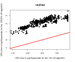
Plot of time in seconds with CS algorithm on the $x$-axis and the LP algorithm from [2] on the $y$-axis. Both algorithms compute approximated solutions for 962 threading instances associated to the template 1ASYA0 from the FROST database. The linear curve in the plot is the line $y=x$. What is observed is a significant performance gap between the algorithms. For example in a point $(x,y)=(0.5,3)$ CS is $10^{2.5}$ times faster than LP relaxation. These results were obtained on an Intel(R) Xeon(TM) CPU 2.4 GHz, 2 GB RAM, RedHat 9 Linux. The MIP models were solved using CPLEX 7.1 solver [7].

Figure 6: Cost-Splitting Relaxation versus LP Relaxation

We conducted the following experiment. For the purpose of this section we chose a set of 12 non-trivial templates. 60 distributions are associated to them. We first computed these distributions using an exact algorithm for solving the underlying PTP problem. The same distributions have been afterwords computed using the approximated solutions obtained by any of the three algorithms here considered. By approximated solution we mean respectively the following: i) for a MIP model this is the solution given by the LP relaxation; ii) for the Lagrangian Relaxation (LR) algorithm this is the solution obtained for 500 iterations (the upper bound used in [3]). Any exit with less than 500 iterations is a sign that the exact value has been found; iii) for the Cost-Splitting algorithm (CS) this is the solution obtained either for 300 iterations or when the relative error between upper and lower bound is less than $0.001$.

We use the MYZ integer programming model introduced in [2]. It has been proved faster than the MIP model used in the package RAPTOR [16] which was well ranked among all non-meta servers in CAFASP3 (Third Critical Assessment of Fully Automated Structure Prediction) and in CASP6 (Sixth Critical Assessment of Structure Prediction). Because of time limit we present here the results from 10 distributions only. Concerning the 1st quartile the relative error between the exact and approximated solution is $3\times 10^{-3}$ in two cases over all 2000 instances and less than $10^{-6}$ for all other cases. Concerning the 3rd quartile, the relative error is $10^{-3}$ in two cases and less than $10^{-6}$ for all other cases.

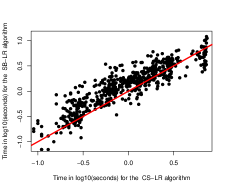
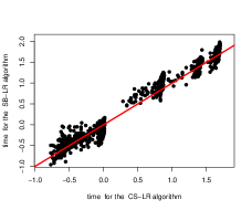
Figure 7: Plot of time in seconds with CS (Cost-Splitting Relaxation) algorithm on the $x$-axis versus LR (Lagrangian Relaxation) algorithm [3] on the $y$-axis concerning score distributions of two templates. Both the $x$-axis and $y$-axis are in logarithmic scales. The linear curve in the plot is the line $y=x$. Left: The template 1ASYA (the one referenced in [3]) has been threaded with 962 sequences. Right: 1ALO_0 is one of the templates yielding the biggest problem instances when aligned with the 704 sequences associated to it in the database. We observe that although CS is often faster than LR, in general the performance of both algorithms is very close.

All 12125 alignments for the set of 60 templates have been computed by the other two algorithms. Concerning the 1st quartile, the exact and approximated solution are equal for all cases for both (LR and CS) algorithms. Concerning the 3rd quartile and in case of LR algorithm the exact solution equals the approximated one in all but two cases in which the relative error is respectively $10^{-3}$ and $10^{-5}$. In the same quartile and in case of CS algorithm the exact solution equals the approximated one in 12119 instances and the relative error is $7\times 10^{-4}$ in only 6 cases.

Obviously, this loss of precision (due to computing the distribution by not always taking the optimal solution) is negligible and does not degrade the quality of the prediction. We therefore conclude that the approximated solutions given by any of above mentioned algorithms can be successfully used in the score distributions phase.

7.3 Cost splitting versus Linear Programming and Lagrangian relaxations

Our third numerical experiment concerns running time comparisons for computing approximated solutions by LP, LR and CS algorithms. The obtained results are summarized on figures 6, 7 and 8. Figure 6 clearly shows that CS algorithm significantly outperforms the LP relaxation. Figures 7 and 8 compare CS with LR algorithm and illustrate that they give close running times (CS being slightly faster than LR). Time sensitivity with respect to the size of the problem is given in Fig. 8.

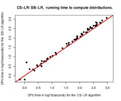
Plot of time in seconds with CS algorithm on the $x$-axis and the LR algorithm on the $y$-axis. Each point corresponds to the total time needed to compute one distribution determined by approximately 200 alignments of the same size. 61 distributions have been computed which needed solving totally 12125 alignments. Both the $x$-axis and $y$-axis are in logarithmic scales. The linear curve in the plot is the line $y=x$. CS is consistently faster than the LR algorithm.

Figure 8: CS versus LR : recapitulation plot concerning 12125 alignments.

8 Conclusion

The results presented in this paper confirm once more that integer programming approach is well suited to solve the protein threading problem. Even if the possibilities of general purpose solvers using linear programming relaxation are limited to instances of relatively small size, one can use the specific properties of the problem and develop efficient special purpose solvers. After studying these properties we propose two Lagrangian approaches, Lagrangian relaxation and cost splitting. These approaches are more powerful than the general integer programming and allow to solve huge instances, with solution space of size up to $10^{77}$, within a few minutes.

The results lead us to think that even better performance could be obtained by relaxing additional constraints, relying on the quality of LP bounds. In this manner, the relaxed problem will be easier to solve. This is the subject of our current work.

This paper deals with the problem of global alignment of protein sequence and structure template. But the methods presented here can be adapted to other classes of matching problems arising in computational biology. Examples of such classes are semi-global alignment, where the structure is aligned to a part of the sequence (the case of multi-domain proteins), or local alignment, where a part of the structure is aligned to a part of the sequence. Problems of structure-structure comparison, for example contact map overlap, are also matching problems that can be treated with similar techniques. Solving these problems by Lagrangian approaches is work in progress.

References

- [1] T. Akutsu and S. Miyano. On the approximation of protein threading. Theoretical Computer Science, 210:261–275, 1999.
- [2] R. Andonov, S. Balev and N. Yanev, Protein Threading Problem: From Mathematical Models to Parallel Implementations, INFORMS Journal on Computing, 2004, 16(4), pp. 393-405
- [3] Stefan Balev, Solving the Protein Threading Problem by Lagrangian Relaxation, WABI 2004, 4th Workshop on Algorithms in Bioinformatics, Bergen, Norway, September 14 - 17, 2004
- [4] D. Fischer, http://www.cs.bgu.ac.il/ dfishcer/CAFASP3/, Dec. 2002
- [5] A. Caprara, R. Carr, S. Israil, G. Lancia and B. Walenz, 1001 Optimal PDB Structure Alignments: Integer Programming Methods for Finding the Maximum Contact Map Overlap Journal of Computational Biology, 11(1), 2004, pp. 27-52
- [6] H. J. Greenberg, W. E. Hart, and G. Lancia. Opportunities for combinatorial optimization in computational biology. INFORMS Journal on Computing, 16(3), 2004.
- [7] Ilog cplex. http://www.ilog.com/products/cplex
- [8] R. Lathrop, The protein threading problem with sequence amino acid interaction preferences is NP-complete, Protein Eng., 1994; 7: 1059-1068
- [9] A. Marin, J.Pothier, K. Zimmermann, J-F. Gibrat, FROST: A Filter Based Recognition Method, Proteins, 2002 Dec 1; 49(4): 493-509
- [10] Marin, A., Pothier, J., Zimmermann, K., Gibrat, J.F.: Protein threading statistics: an attempt to assess the significance of a fold assignment to a sequence. In Tsigelny, I., ed.: Protein structure prediction: bioinformatic approach. International University Line (2002)
- [11] T. Lengauer. Computational biology at the beginning of the post-genomic era. In R. Wilhelm, editor, Informatics: 10 Years Back - 10 Years Ahead, volume 2000 of Lecture Notes in Computer Science, pages 341–355. Springer-Verlag, 2001.
- [12] G. Lancia. Integer Programming Models for Computational Biology Problems. J. Comput. Sci. & Technol., Jan. 2004, Vol. 19, No.1, pp.60-77
- [13] R.H. Lathrop and T.F. Smith. Global optimum protein threading with gapped alignment and empirical pair potentials. J. Mol. Biol., 255:641–665, 1996.
- [14] G. L. Nemhauser and L. A. Wolsey. Integer and Combinatorial Optimization. Wiley, 1988.
- [15] J.C. Setubal, J. Meidanis, Introduction to computational molecular biology, 1997, Chapter 8: 252-259, Brooks/Cole Publishing Company, 511 Forest Lodge Road, Pacific Grove, CA 93950
- [16] J. Xu, M. Li, G. Lin, D. Kim, and Y. Xu. RAPTOR: optimal protein threading by linear programming. Journal of Bioinformatics and Computational Biology, 1(1):95–118, 2003.
- [17] Y. Xu and D. Xu. Protein threading using PROSPECT: design and evaluation. Proteins: Structure, Function, and Genetics, 40:343–354, 2000.
- [18] N. Yanev and R. Andonov, Parallel Divide and Conquer Approach for the Protein Threading Problem, Concurrency and Computation: Practice and Experience, 2004; 16: 961-974
- [19] V. Poirriez, R. Andonov, A. Marin and J-F. Gibrat, FROST: Revisited and Distributed In IPDPS ’05: Proceedings of the 19th IEEE International Parallel and Distributed Processing Symposium (IPDPS’05) - Workshop 7, 2005, IEEE Computer Society