Clone size distributions in networks of genetic similarity

Abstract

We build networks of genetic similarity in which the nodes are organisms sampled from biological populations. The procedure is illustrated by constructing networks from genetic data of a marine clonal plant. An important feature in the networks is the presence of clone subgraphs, i.e. sets of organisms with identical genotype forming clones. As a first step to understand the dynamics that has shaped these networks, we point up a relationship between a particular degree distribution and the clone size distribution in the populations. We construct a dynamical model for the population dynamics, focussing on the dynamics of the clones, and solve it for the required distributions. Scale free and exponentially decaying forms are obtained depending on parameter values, the first type being obtained when clonal growth is the dominant process. Average distributions are dominated by the power law behavior presented by the fastest replicating populations.

, , , ,

1 Introduction

Biological systems have always been quoted as archetypes of complexity. Modern network approaches [1, 2, 3, 4, 5] have provided useful insight when applied to many of them, ranging from protein interaction networks [6] to food webs [7, 8]. One of the most fundamental processes through which organisms interact is that of genetic interactions, which conforms the basis for evolutionary processes. The need to represent such processes in network structures more complex than simple trees is beginning to be appreciated [9], but modern network paradigms are not yet widely used to understand genetic relationships among individuals, communities or species.

In this paper we overview the construction of networks of genetic similarity. They are useful tools to represent and analyze the genetic structure of the different genotypes in a biological population. We use the method to organize genetic data from a Mediterranean marine plant, Posidonia oceanica. Then, we move from a static depiction of these networks to the exploration of the dynamics that has shaped them. A network characteristic that turns out to be accessible to mathematical analysis is the degree distribution of a particular case of similarity network. Such particular degree distribution is directly related to the clone size distribution in the population. We construct a dynamical model for the population dynamics and solve it for the required distributions. Scale free and exponentially decaying forms are obtained depending on parameter values. Averages over several populations, however, are dominated by the power-law behavior displayed by the fastest clonally growing populations.

2 Networks of genetic similarity

We illustrate our approach with genetic data obtained by genotyping specimens of Posidonia oceanica, a marine plant living in the coastal waters of the Mediterranean sea [10]. An important characteristic of this organism is that it is a clonal plant, meaning that in addition to the standard sexual reproduction involving the flowers in different shoots, the plant also reproduces by growing new shoots or ramets that are genetically identical to the existing ones. The process is called clonal reproduction, and the set of ramets generated in this way starting from an initial one form a single clone. Seeds generated by sexual reproduction start new clones. At short distances, the members of a clone are physically connected by a common rhizome. Physical connection between distant ramets can be interrupted by a number of reasons (for example the death of a part of the intermediate rhizome). From our genetic data we will still identify them as members of the same clone because they share the same genotype. Mutations, however, can occur during the process of clonation. It is customary to consider these mutants with slightly different genotypes, and the lineages arising clonally from them, as part of the same original clone. In this paper, however, we find convenient to take the operational definition of a clone as the set of ramets with identical genotype. Within this point of view, mutants are considered to be founders of new clones.

Our data set comes from about 40 ramets sampled from each of 38 populations across the Mediterranean. For each ramet, the genetic data consist in the number of microsatellite repetitions at seven loci. Microsatellites [11] are highly variable portions of the genome commonly used for intraspecific studies. They contain a motif consisting of a short sequence of bases which is repeated for a variable number of times in genetically different individuals. Additional details on the genetic dataset can be found in Refs. [12, 13]. In Ref. [14] we introduced a suitable measure of genetic dissimilarity among the ramets in the data set. This genetic distance between a pair of ramets is defined as the difference (in absolute value) in the number of motif repetitions present at a particular genome locus of the two ramets, summed over the seven analyzed loci. In this way genetically identical individuals (belonging to the same clone) are at zero distance, and biological processes can be associated with different distances; for example there is a characteristic mean genetic distance between parents and offspring generated by sexual reproduction [14].

Once a matrix of genetic distances has been constructed, one can in principle apply the tools of classical phylogenetics [15] to analyze genetic and evolutionary relationships among the genotypes. Nevertheless, the fact that we are dealing with intraspecific data and the coexistence of sexual and clonal modes of reproduction in Posidonia challenges the applicability of these methods. Aiming at addressing these issues, networks of genetic similarity have been introduced in [14]. In the same spirit as in correlation networks [16, 17, 18], a similarity threshold is introduced in which the individual ramets are represented by nodes and there is a link between them if their distance is smaller than the threshold, i.e. if they are more similar than the threshold value. This gives a sequence of networks, one for each threshold value. Figure 1 displays examples of similarity networks at different threshold values for the ramets sampled from a population in Es Caló de s’Oli (Formentera island, Spain). Connectivity increases fast around a threshold value of 30, which is identified in this particular population with the mean distance arising between parents and sexual offspring (outcrossing distance).

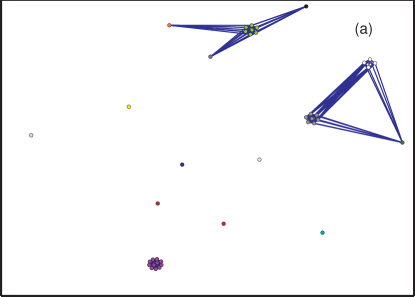
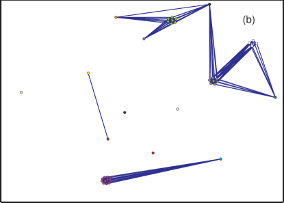
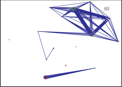
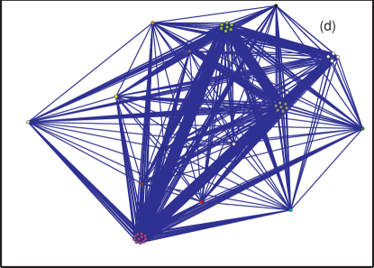
Figure 1: Similarity networks of ramets from es Caló de s’Oli (island of Formentera, Spain), at different similarity threshold values: a) 20, b) 27, c) 34, and d) $>$92 (which leads to a fully connected network). Note the groups of nodes, plotted close together, which are fully connected subgraphs and remain fully connected for all values of the threshold. They are the clones.

A standard characterization of the topology of a network is the connectivity degree distribution $P(x)$. It is the proportion of nodes in a network with a given number $x$ of links. Because of the limited amount of data, the networks are rather small and the degree distributions from each of them are noisy and highly variable. Patterns are clearer when averaging the degree distributions of the 38 sampled populations. Figure 2 shows this averaged distribution at two different values of the threshold. When the threshold takes a value of the order of the mean outcrossing distance (Fig. 2a), the degree distribution is essentially flat, although large statistical fluctuations still remain. To our knowledge, this kind of flat degree distribution has only been reported previously in the context of food webs [8] (displayed there as accumulated distributions which vary linearly).

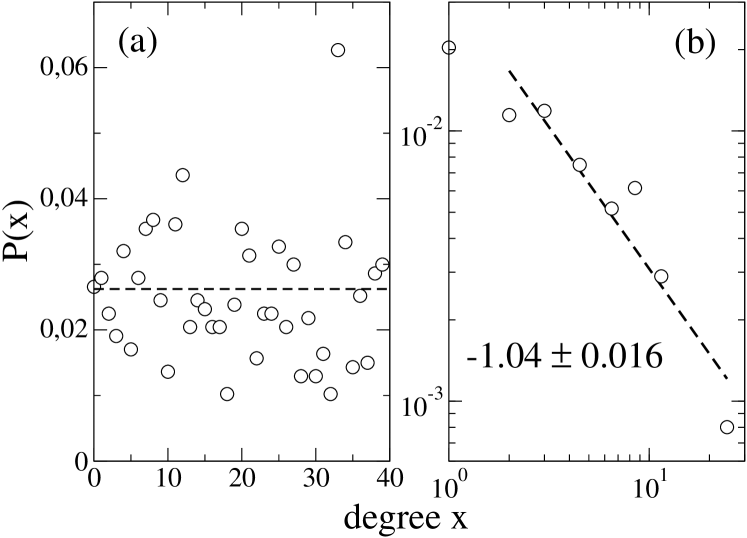
Figure 2: Degree distributions, averaged over all the sampled populations. a) For networks at threshold 30, which is the most abundant non zero distance in the data set and of the order of the mean outcrossing distance. Distribution is roughly uniform. b) Zero threshold, so that only clones remain connected. Data have been binned by the data threshold method as presented in Ref. [19]. The distribution is fitted by a power law with the exponent indicated.

At threshold zero only identical ramets, i.e. pertaining to the same clone, remain linked. Fig. 2b shows the averaged degree distribution in this case. The amount and range of the data are small, but the power-law fit (suggested by the theoretical arguments discussed in the following) indicates that they are compatible with a degree distribution of the scale-free type. It turns out that, for this zero-threshold case, the shape of the distribution can be understood in terms of a model for the population dynamics. The crucial point is to recognize that there is a relationship between the degree distribution at zero threshold $P_{0}(x)$, and the distribution of clone sizes, i.e., the number $H_{K}$ of clones having a number of ramets $K$. This arises from the fact that clones are fully connected subgraphs, so that in a clone of $K$ ramets, each ramet has $K-1$ links. Introducing $M(x)\equiv NP_{0}(x)$ as the number of nodes with $x$ links in a network of $N$ ramets, the relationship is

$$H_{K}=\frac{1}{K}M(K-1)$$ (1)

Thus the topological problem of calculating this degree distribution becomes a question in population dynamics: the calculation of clone sizes. This last question falls within the general category of ‘growth-death-innovation’ processes related to the models of Yule [20], Simon [21] and others, as summarized in Ref. [22]. We devote the rest of the paper to build and solve a stochastic model of that type from which the clone size distribution and other useful quantities can be analytically extracted. We stress that the topological structure of the network at similarity threshold zero is very simple: it consists of disjoints sets (the clones) of nodes which remain internally fully connected. Thus, standard network descriptors have rather trivial values in this case (for example the clustering coefficient is always one, independently of degree). This is why we focus on the degree distribution, and in the number of connected components (given by the richness defined below), as the only nontrivial quantities characterizing the network at vanishing threshold.

3 Modelling population and clone dynamics

A plant population (a meadow) consists of a variable number $N=N(t)$ of ramets. We label the different genotypes in the population –the different clones– with numbers $j$, $j=1,2,...,G$, so that $G$ is the richness of the population, i.e. the number of different clones. $K_{j}$ is the number of ramets forming clone $j$. We have $N=\sum_{j=1}^{G}K_{j}$. The histogram $H_{K}=\sum_{j=1}^{G}\delta_{K,K_{j}}$ counts how many clones of size $K$ are in the population. We have

$$G=\sum_{K=1}^{\infty}H_{K}\ ,\$$ (2)

and

$$N=\sum_{K=1}^{\infty}KH_{K}$$ (3)

As a major simplification in our approach, we neglect any difference among the ramets arising from their age, genetic content, or integration into big or small clones. Thus all ramets are described by the same parameters of mortality, reproduction, etc. Additionally we consider a well mixed population so that spatial effects are not taken into account. The local density is the same everywhere and simply proportional to the population size $N$. Finally, we do not take into account any possible seasonal modulation of the different rates. The limitations introduced in our modelling approach by these simplifications will be briefly discussed in Section 4.

We now introduce the elementary processes occurring in our stochastic model (mortality, clonal and sexual reproduction, mutation, and migrations). They are considered to be independent events occurring at Poisson times:

• Death at rate $d$. Each ramet has a probability $d$ per unit of time of dying. In Posidonia oceanica mortality is not strongly dependent on population density, so that we could take its value to be a constant. But in order to keep the model general enough we include some competition for resources in terms of a mortality that increases with population size: $d=d(N)=d_{0}+\nu N$.

• Clonal reproduction at rate $c$. The quantity $c$ is the probability of ramet clonal reproduction per unit of time, which may be density dependent: $c=c(N)=\max\left[0,c_{0}\left(1-N/N_{s}\right)\right]$. $N_{s}$ is the number of ramets in the population beyond which clonal reproduction becomes impossible. This saturation effect is relevant in Posidonia populations, and fixes a maximum density for the meadow. The max function is needed to avoid negative probabilities. If the dynamics keeps $N$ sufficiently below $N_{s}$ we can approximate $c\approx c_{0}\left(1-N/N_{s}\right)$.

• Mutations with probability $p_{m}$. In the process of clonal reproduction a mutation can occur with probability $p_{m}$. We assume that each mutant genotype is different from the ones already present in the population, and thus founds a new clone. We neglect the possibility of mutation backwards to the original genotype.

• Sexual reproduction at rate $s$. At first sight, the number of births arising from sexual reproduction should be proportional to the product of the number of male and female flowers in the population, and thus roughly to $N^{2}$. But in Posidonia populations, as well as in other plant species, pollen is produced in great abundance so that reproduction is rather proportional to the number of females. Since Posidonia flowers are hermaphrodite, this equals the total number of flowers, that we assume to be proportional to the number of ramets $N$. Nevertheless, we keep the modelling at a general level and include both a linear and a quadratic dependence on $N$ for the number of sexual births, which implies a sexual reproduction rate per ramet of $s=s(N)=s_{0}+\epsilon N$. Sexual reproduction produces unique individuals as a consequence of the random recombination of the progenitor’s genomes. Thus, each newborn founds a new clone. Sexual reproduction in plants is strongly seasonal, but we consider here the process as occurring continuously in time.

• Migration, $I$. Migration process (transport of seeds or broken ramets by marine currents, animals or ships) will only renormalize the death parameters $d_{0}$ and $\nu$ when they imply a loss from the population. These changes will not be explicitly written down. When there is input of ramets from outside the population we assume that immigrants are genetically distinct from any of the local clones, so that they also found new clones on arrival. We will call $I$ the number of immigrants entering the population per unit of time.

Summarizing the modelling parameters, we have the basic death, clonation, and sexual reproduction rates of ramets at low densities ($d_{0}$, $c_{0}$, and $s_{0}$, respectively), the modifications to these rates from interactions ($\nu$, $N_{s}$, and $\epsilon$, respectively), the probability of mutation while cloning ($p_{m}$), and the immigration rate ($I$). There are strong differences among different populations, leading to rather different network structures [14]. This reflects the fact that they are in very different states, some of them healthy, many of them receding, and are subjected to a large variety of environmental parameters and pressures. Accordingly, we will postpone the discussion on the election of numerical values for the different parameters until Section 4, in which we will argue that average quantities such as the distributions plotted in Fig. 2 are dominated by populations having particular parameter values. Until then we keep the discussion general, using arbitrary parameter values, which is also convenient for developing a formalism that can be later applied to species different from the one considered here.

3.1 Population size rate equation

It is simple to write down the rate equation for the time evolution of the expected population size $N$. Neglecting all fluctuations and correlations, and taking into account that mutations do not alter the number of individuals, the net growth rate per ramet is $\gamma_{T}=c(N)+s(N)-d(N)$, so that:

$$\dot{N}=\left(c(N)+s(N)-d(N)\right)N+I=\beta N\left(1-\frac{N}{N_{c}}\right)+I\ ,$$ (4)

where $\beta\equiv\left(c_{0}+s_{0}-d_{0}\right)$ is the maximum population growth rate, and we have introduced the carrying capacity $N_{c}$ from the relation

$$\frac{\beta}{N_{c}}\equiv\frac{c_{0}}{N_{s}}+\nu-\epsilon$$ (5)

or

$$N_{c}=\frac{\beta N_{s}}{c_{0}+N_{s}(\nu-\epsilon)}\ .$$ (6)

In the absence of migration, $I=0$, Eq. (4) is just the logistic equation. If $\beta>0$ any initial condition approaches the saturation value $N_{c}$. Solutions from small initial values of $N$ have an initial exponentially growing phase ($N\approx N_{0}e^{\beta t}$). If $\beta<0$ the solution decays towards zero (extinction), exponentially if $N$ is sufficiently smaller than $N_{c}$. We notice however that stochastic fluctuations, neglected in Eq. (4), will be important when the population is small.

3.2 Expected clone size

Let us focus on clone $j$ of size $K_{j}=K_{j}(t)$ (again we will neglect its statistical fluctuations). Sexual reproduction, mutations and immigrants do not change it. Thus

$$\dot{K}_{j}(t)=\gamma_{c}K_{j}(t),$$ (7)

with $\gamma_{c}(N)\equiv g_{c}(N)-d(N)$. We call $g_{c}(N)\equiv(1-p_{m})c(N)$ the clonal growth rate, and $\gamma_{c}$ is a net clonal growth rate.

On average, sexual reproduction, mutations and immigration increase the richness $G$ by starting an amount $\left(p_{m}c(N)+s(N)\right)N+I$ of new clones of size 1 per unit of time. As a consistency check, one can see that the sum of Eq. (7) over all clones ($\sum_{j=1}^{G}K_{j}(t)=N(t)$), with the addition of the new ones, leads to the population equation (4).

Once $N(t)$ is obtained from (4), Eq. (7) can be integrated exactly. The simplest situation corresponds to $\nu=\epsilon=c_{0}/N_{s}=0$, so that ramets do not interact (in this case Eq. (7) is exact for the average clone size even in the presence of fluctuations). Then, $\gamma_{c}$ is a constant in time ($\gamma_{c}=(1-p_{m})c_{0}-d_{0}$), and $K_{j}(t)=K_{j}(0)e^{\gamma_{c}t}$. We note that $\gamma_{c}<\gamma_{T}$, so that clones will only grow on average when the total population is growing fast enough. It is interesting to note that the total population can be growing while on average each existing clone is decreasing in size. A similar situation occurs for interacting ramets when $N(t)$ is constant in time (this happens when $N$ has attained its saturation value, which in the absence of immigration is $N=N_{c}$). In this case $K_{j}(t)=K_{j}(0)e^{\gamma_{c}t}$, with $\gamma_{c}=\gamma_{c}(N_{c})<0$. On average, existing clones will decrease in size until dying. In the mean time, mutations, sex and immigration will introduce clones of size one (single ramets), and this together with stochastic fluctuations will maintain a steady state distribution of clone sizes peaked at small values.

3.3 Clone size distribution

The next step is to estimate the whole clone size distribution $H_{K}$ in the population. By balancing the different rates, we find that the expected value of that distribution is ruled by:

$$\frac{d}{dt}H_{K}(t) = g_{c}\left((K-1)H_{K-1}(t)-KH_{K}(t)\right)$$

$$+ d\left((K+1)H_{K+1}(t)-KH_{K}(t)\right)\ ,\ \ \ K>1$$

$$\frac{d}{dt}H_{1}(t) = I+hN(t)-g_{c}H_{1}(t)+d\left(2H_{2}(t)-H_{1}(t)\right)\ .$$ (9)

This mean field description becomes exact when ramets do not interact. The increase in $H_{1}(t)$, the number of clones consisting of a single ramet, arises from immigration $I$ and from mutants and sexual offspring: $h=h(N)\equiv p_{m}c(N)+s(N)=\gamma_{T}-\gamma_{c}$. This quantity $h$ can be thought as the amount of innovation, since it gives the rate at which new genotypes are produced by the system. Note that $N(t)$ in Eq. (9) is not an independent variable, but it is related to all the $H$’s by Eq. (3). Thus the single-ramet population $H_{1}$ plays a special role since it interacts with all the clone-size groups. Equation (4), which is closed for $N(t)$, is recovered from Eqs. (3) and (LABEL:Hk)-(9). If one uses first this equation to find $N(t)$, one of the equations in (LABEL:Hk)-(9) becomes redundant.

From Eqs. (LABEL:Hk)-(9) one can obtain an equation for the richness (2):

$$\frac{d}{dt}G(t)=I+hN(t)-dH_{1}(t)\ .$$ (10)

We analyze now Eqs. (LABEL:Hk)-(9) in some particular cases. For simplicity we neglect immigration: $I=0$, and we only address the situations of noninteracting ramets ($\nu=c_{0}/N_{s}=\epsilon=0$), and of interacting ramets in a constant population $N(t)=N_{c}$. In these cases, (LABEL:Hk) are effectively linear equations with coefficients constant in time, and the explicit time dependence of $N(t)$ in (9) can be written as $N(t)=N_{0}e^{\gamma_{T}t}$. In the noninteracting case $\gamma_{T}=\beta$, $h=p_{m}c_{0}+s_{0}$, and we can have either a growing population if $\beta=c_{0}+s_{0}-d_{0}>0$ or a decaying one if $\beta<0$. Note that this description also applies to the interacting ramet case when the population is small enough, because the interaction terms become negligible when $N\approx 0$. In the interacting constant population case $\gamma_{T}=0=h+g_{c}-d$ and $N_{0}=N_{c}$

In all cases we search for solutions of the type

$$H_{K}(t)=F_{K}e^{rt}\ .$$ (11)

We see from substitution in Eq. (3) that

$$N(t)=e^{rt}\sum_{K=1}^{\infty}KF_{K}\equiv e^{rt}R$$ (12)

so that necessarily $r=\gamma_{T}$. The sum in Eq. (12), which we call $R$, should converge to $N_{0}$ or $N_{c}$.

Substituting Eq. (11) into (LABEL:Hk)-(9) we get

$$\gamma_{T}F_{K} = g_{c}(K-1)F_{K-1}+d(K+1)F_{K+1}-(g_{c}+d)KF_{K}\ \ ,\ \ \ \ K>1$$ (13)

$$\gamma_{T}F_{1} = hR-(g_{c}+d)F_{1}+2dF_{2}$$ (14)

Equation (13) is a second order linear recurrence, having in principle two independent solutions. The point is that only one of them will satisfy the constraint (12) with a convergent sum $R$. Fixing $N_{0}$ or $N_{c}$ ($=R$) then normalizes and completely determines the distribution.

We find the asymptotic behavior for large $K$ of the two possible solutions of Eq. (13) by substituting the ansatz

$$F_{K}\sim\frac{\theta^{K}}{K^{z}}\ .$$ (15)

The first two terms in an expansion in powers of $K^{-1}$ determine two independent solutions:

$$A:\hskip 28.45274pt \theta=1\ ,\ \ z=1+\frac{\gamma_{T}}{\gamma_{c}}=2+\frac{h}{\gamma_{c}}$$ (16)

$$B:\hskip 28.45274pt \theta=\frac{g_{c}}{d}\ ,\ \ z=1-\frac{\gamma_{T}}{\gamma_{c}}=-\frac{h}{\gamma_{c}}$$ (17)

Figure 3: a) Exponent z as a function of net clonal growth $\gamma_{c}$. $d=1$ and $h=0.25$. The place where $\gamma_{T}=0$, giving $z=1$, is indicated. b) Clone distributions. $d=1$, $h=0.25$, and $\gamma_{c}$ increasing from top to bottom: $g_{c}=0.6,0.75,0.95,1.05,1.15$. The upper curve is the limit case $g_{c}>>h$, leading to $z=2$. The line labelled $\gamma_{T}=0$ ($g_{c}=0.75$) is the exact solution given by Eq. (18), and the other curves have the proper asymptotic behavior but have been arbitrarily shifted vertically for clarity. For $\gamma_{c}>0$ (three upper lines) solution A (Eq. (16)) gives a power law behavior with exponent $z$. For $\gamma_{c}<0$ (three lower curves) the exponent in solution B (Eq. 17)) gives only a pre-asymptotic power law behavior, being the final decay of exponential type.

The values of the exponent $z$ depend on the ratio between the net growth $\gamma_{T}$ (or of the innovation $h$) and the clonal net growth $\gamma_{c}=g_{c}-d$. We analyze separately the following three cases: $\gamma_{T}=0$, $\gamma_{c}<0$ (which includes cases with $\gamma_{T}>0$ and $\gamma_{T}<0$), and $\gamma_{c}>0$ (which only happens when $\gamma_{T}>0$). When $\gamma_{c}=0$ the ansatz (15) is not appropriate.

• Constant population size ($\gamma_{T}=0$). Since $h+g_{c}-d=0$ we have $g_{c}<d$, and the size of a given clone is decreasing on average. Solution A (Eq. (16)) makes the sum in (12) to diverge and B is the correct solution. It turns out that it gives not only the asymptotic behavior, but an exact solution for all $K$, the so-called logarithmic distribution:

  $$H_{K}(t)=\frac{hN_{c}}{g_{c}}\left(\frac{g_{c}}{d}\right)^{K}\frac{1}{K}=N_{c}\left(\frac{d}{g_{c}}-1\right)\left(\frac{d}{g_{c}}\right)^{-K}\frac{1}{K}\ .$$ (18)

  As expected, this is concentrated at small clone sizes, with a quasi-exponential decay at large $K$. When the mutation and sex rates are small (so that $g_{c}$ approaches $d$) the range of existing clone sizes becomes larger. In [23] this exact solution is also found for a related set of equations in the context of the ‘simple BDIM model’ of protein evolution, and its stability is proven. Thus, arbitrary initial distribution of clones will converge at long times towards Eq. (18) when the population has reached a constant value.

  The richness can be calculated from (10). The relative richness $v$ becomes:

  $$v\equiv\frac{G}{N_{c}}=\left(1-\frac{d}{g_{c}}\right)\log\left(1-\frac{g_{c}}{d}\right)\ .$$ (19)

  This relative richness is a decreasing function of $g_{c}/d$, from a maximum value in the case of maximum mutations and sex ($g_{c}/d\approx 0$, $v\approx 1$) to a vanishing value in the case of minimum mutations and sex ($g_{c}/d\approx 1$, $v\approx 0$).

• Decreasing average clone size ($\gamma_{c}=g_{c}-d<0$). This case includes situations in which population is decreasing ($\gamma_{T}=\beta<0$), but also cases in which there is net growth ($\gamma_{T}=\beta>0$) but not enough of the purely clonal type. The sum in (12) diverges for solution A (Eq. (16)) and again B (Eq. (17)) gives the correct asymptotic behavior. Thus there are solutions to (LABEL:Hk)-(9) that behave at large $K$ as

  $$H_{K}(t)\sim\frac{e^{\beta t}}{K^{z}}\left(\frac{g_{c}}{d}\right)^{K}$$ (20)

  with

  $$z=1-\frac{\beta}{\gamma_{c}}=1-\frac{c_{0}-d_{0}+s_{0}}{c_{0}-d_{0}-p_{m}c_{0}}\ .$$ (21)

  The asymptotic behavior is again quasi-exponential, with faster decay for smaller $g_{c}/d$. As if trying to compensate for this increased steepness, the exponent of $K$, $-z$, becomes less negative when decreasing $g_{c}/d$ (see Fig. 3a), starting from a divergent value when $g_{c}\approx d$, crossing to $-z=-1$ when $\beta=0$ (formally coinciding with the solution for constant population), and approaching $z=0$ when $g_{c}/d\rightarrow 0$. Note that, despite this asymptotic behavior, there is a pre-asymptotic power law behavior with exponent $z$, which can be noticeable (see Fig. 3b, third curve from bottom) when $\gamma_{c}$ is close to zero.

• Growing average clone size ($\gamma_{c}=g_{c}-d>0$). This situation requires a net population growth ($\gamma_{T}=\beta>\gamma_{c}>0$). In this case solution B (Eq. (17)) is not normalizable and the power law solution A (Eq. (16)) is the only acceptable asymptotic behavior at large $K$:

  $$H_{K}(t)\sim\frac{e^{\beta t}}{K^{z}}$$ (22)

  with

  $$z=1+\frac{\beta}{\gamma_{c}}=1+\frac{c_{0}-d_{0}+s_{0}}{c_{0}-d_{0}-p_{m}c_{0}}\ .$$ (23)

  This result coincides with the one in Refs. [24, 25] for family name distributions obtained from a discrete-time model of growing families. It reduces to the classical result of Simon [21], explaining the Zipf’s observations on the growth of cities, if $d=0$ so that $z=2$. The clone distribution of a growing population reaches a power law with the exponent related to the quotient between the net growth and the net clonal growth. Starting from the less negative exponent, the one with $z=2$, the power law has a more and more negative exponent when $g_{c}$ approaches $d$ from above, so that the clone distribution becomes more concentrated, until reaching $g_{c}=d$. Numerical simulations in Refs. [24, 25] show (within their discrete model) that the state given by Eq. (22) is actually approached at long times, although long transients can occur.

4 Discussion and perspectives

We have found that, within the hypothesis of our model, clone distributions decay at large $K$ either as a power law or exponentially (with power law corrections). The first situation occurs when clones are growing on average, which requires a global population growth, and the second when clones shrink on average.

Figure 4a displays the observed clone distribution averaged over all sampled plant populations, obtained from the degree distribution in Fig. 2 by using Eq. (1) (or equivalently by directly counting the clones in the populations and averaging the resulting histograms). The asymptotic behavior is consistent with a power law of exponent $z\approx 2.1$ (for completeness, however, and given the small range of the data, we show also in the inset a semilogarithmic plot of the same points which gives only a slightly worse representation). The appropriateness of the power law fitting seems to imply that data are better explained by a model in which clones are growing, which needs population grow, and that there is a small proportion of sexual reproduction and mutations with respect to clonal growth.

Although certainly it is realistic to have a rate of accurate clonal reproduction much larger than sexual or mutational rates, most of the studied populations were in recession rather than growing, and some of them in serious danger of disappearance. Given the limitation in number and range of the data presented in Fig. 4a, we can not exclude that the sampled clone sizes are not in the asymptotic range addressed by the theory, or the possibility of functional forms other than power laws, but the proximity of the fitted slope to the particular value $z=2$ suggest us the following argument: We believe that data in Fig. 4 do not reflect a generally growing population state, but rather a mixed state in which some populations are stable or receding, but with the average clone distribution dominated by a few populations in a clonally growing state. To check this we plot in Fig. 4b a set of distributions of types (20) and (22). They have been generated by choosing units of time such that $d=1$, fixing $h=0.05$, and randomly generating values of $g_{c}$ from a uniform distribution in $[0.0,1.6]$. All the distributions are normalized to the same value $\sum_{1}^{\infty}KH_{K}=N=40$ as reflecting that the same number of ramets has been sampled from each population independently of its true total size. The mean value of $g_{c}$ is 0.8, so that the mean values of both the net growth and the clonal net growth are negative. Nevertheless, the asymptotic behavior of the average distribution is a power law dominated by the particular population which turns out to be growing and having the value of $z$ closest to $z=2$.

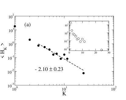
Figure 4: a) Clone distribution averaged over the 38 sampled populations. Data are binned as in Fig. 2b, and presented in doubly logarithmic scale with a power-law fit leading to $z\approx 2.1$. The inset shows the same data in semilogarithmic scale. b): Thin continuous lines are 38 distributions $H_{K}$ of the type A or B, with $d=1$, $h=0.05$, and random values of $g_{c}$ as explained in the text. Thick continuous line is their average $<H_{K}>$, arbitrarily displaced vertically for clarity. Its asymptotic behavior at large $K$, $K^{z}$, is indicated by a dashed line and is the power law corresponding to the largest value of $g_{c}$ in the averaged sample. In the particular set averaged here, it is $g_{c}\approx 1.54$, leading to $z\approx 2.09$.

The dominance of the populations with the highest clonal net growth (the fastest replicators) would not be restricted to interpopulation averages: As soon as there is some diversity inside a population (different clones differ in size, genotype, location, age, …) the same arguments imply that the subpopulation with the highest clonal net growth would dominate the large size part of the clone distribution in a meadow. We expect thus a bias in the observed clone distributions towards power laws characterized by exponents $z$ larger than but close to $z=2$ (and associated degree distributions $P_{0}(x)$ behaving asymptotically as $x^{-q}$, with $q$ larger than but close to $q=1$). Testing these expectations for Posidonia meadows should wait until the availability of more abundant sets of intrapopulation genetic data, to achieve the necessary statistical power.

Along this paper we have defined clones as sets of genetically identical ramets. Our results can be directly applied to clones defined as sets of ramets arising from clonal reproduction, i.e. considering that both identical ramets and their mutants pertain to the same clone. Size distributions and the rest of properties in Eqs. (18)-(23) are obtained for these clones containing several genotypes simply by putting $p_{m}=0$ in the corresponding formulae, since in this way mutants are counted together with the perfect clones instead of with the sexual newborns. The innovation parameter $h$ is reduced and then the new size distributions are slightly more heavy tailed.

We note that, at the modelling level, sexual reproduction enters just as one more contribution to the innovation parameter $h$. The same role is played by mutations or any other process generating new genotypes from old ones. Thus we expect our approach and results to be applicable to other types of organisms with or without sexual reproduction capabilities, but having an appropriate source of innovation such as mutation.

Several simplifying assumptions limit the generality of our model. Consequences of relaxing the assumption of complete equivalence of the ramets inside the same population have been mentioned before. Spatial effects have also been neglected. Although the assumption of perfect mixing may be justified for the sexual mode of reproduction in populations of sufficiently small extent, clonal growth is an inherently local process. It may happen that, although the mean field density could be small and then not limiting the growth, ramets could be spatially concentrated and competition will make growth smaller than expected. In addition, growth occurs mainly on the periphery of the clones [26]. Associated with these spatial effects are the consequences of statistical fluctuations, enhanced by the discrete nature of individual ramets and mostly neglected in the present work. Fluctuations should be important at least close to the boundary to extinction regimes [27]. We believe that a first consequence of all these effects would be a shift of effective growth rates towards lower values, but taking them properly into account would require extensive computer simulation. An additional complication is that, very likely, any long lived meadow has suffered periods of growth, periods of enhanced mortality, etc. The distributions observed presently in the different populations are probably complicated transient states resulting from all the past history. The impact of time-dependent parameters should be addressed to have a complete description of the processes shaping clone distributions and in general the genetic structure of the populations. This temporal variability, together with the consideration of explicit space dependence will be the subject of future work.

Finally, the focus of this paper has been on the clone subgraphs, structures with a rather peculiar structure. Dynamical modelling of the ecological processes shaping the whole network of genetic similarity of a population remains an open challenge.

References

- [1] S.H. Strogatz, Exploring complex networks, Nature 410 (2001) 268-276.
- [2] R. Albert, A.-L. Barabási, Statistical mechanics of complex networks, Rev. Mod. Phys. 74 (2002) 47-97.
- [3] S. N. Dorogovtsev, J. F. F. Mendes, Evolution of networks, Adv. Phys. 51 (2002) 1079-1187.
- [4] M.E.J. Newman, The structure and function of complex networks, SIAM Review 45 (2003) 167-256.
- [5] S. Boccaletti, V. Latora, Y. Moreno, M. Chavez and D.-U. Hwang, Complex networks: Structure and dynamics, Phys. Rep. 424 (2006), 175-308.
- [6] H. Jeong, S.P. Mason, A.-L. Barabási and Z.N. Oltvai, Lethality and centrality in protein networks, Nature 411 (2001) 41-42.
- [7] R.J. Williams, E.L. Berlow, J.A. Dunne, A.-L. Barabási and N.D. Martínez, Two degrees of separation in complex food webs, Proc. Nat. Acad. Sci. USA 99 (2002) 12913-12916.
- [8] J.A. Dunne, R.J. Williams and N.D. Martínez, Food-web structure and network theory: The role of connectance and size, Proc. Nat. Acad. Sci. USA 99 (2002) 12917-12922.
- [9] D. Posada and K.A. Crandall, Intraspecific gene genealogies: trees grafting into networks, Trends Ecol. Evol. 16 (2001) 37-45.
- [10] A.W.D. Larkum, R.J. Orth, C.M. Duarte , Seagrasses: Biology, Ecology and Conservation (Springer-Verlag, Berlin, 2006).
- [11] D.B. Goldstein, D.D. Pollock, Launching microsatellites: a review of mutation processes and methods of phylogenetic interference, J Hered. 88 (1997) 335-342.
- [12] F. Alberto, L. Correia, S. Arnaud-Haond, C. Billot, C.M. Duarte, E. Serrão, New microsatellite markers for the endemic Mediterranean seagrass Posidonia oceanica, Mol. Ecol. Notes 3 (2003) 253-255.
- [13] S. Arnaud-Haond, F. Alberto, S. Teixeira, G. Procaccini, E. Serrão, C.M. Duarte, Assessing genetic diversity in clonal organisms: low diversity or low resolution? Combining power and cost-efficiency in selecting markers, J. Hered. 96 (2005) 434-440.
- [14] A. F. Rozenfeld, S. Arnaud-Haond, E. Hernández-García, V. M. Eguíluz, M. A. Matías, E. Serrão and C. M. Duarte, Spectrum of genetic diversity and networks of clonal plant populations, arXiv e-print q-bio.PE/0605050 (2006).
- [15] J. Felsenstein, Inferring Phylogenies (Sinauer Associates, Sunderland, 2003).
- [16] J.-P. Onnela, A. Chakraborti, K. Kaski, J. Kertész and A. Kanto , Dynamics of market correlations: Taxonomy and portfolio analysis, Phys. Rev. E 68 (2003) 056110.
- [17] V.M. Eguíluz, D.R. Chialvo, G.A. Cecchi, M. Baliki and A.V. Apkarian , Scale-free brain functional networks, Phys. Rev. Lett. 94 (2005) 018102.
- [18] K. Rho, H. Jeong and B. Kahng, Identification of lethal cluster of genes in the yeast transcription network, Physica A 364 (2006) 557-564.
- [19] Ch. Adami and J. Chu, Critical and near critical branching processes, Phys. Rev. E 66 (2002) 011907.
- [20] G.U. Yule, A mathematical theory of evolution, based on the conclusions of Dr. J.C. Willis, F.R.S., Phyl. Trans. Roy. Soc. London B 213 (1925) 21-87 .
- [21] H.A. Simon, On a class of skew distribution functions, Biometrika 42 (1955) 425-440.
- [22] M.V. Simkin, V.P. Roychowdhury, Re-inventing Willis, arXiv e-print physics/0601192 (2006).
- [23] G.P. Karev, Y.I. Wolf, A.Y. Rzhetsky, F.S. Berezovskaya, E.V. Koonin, Birth and death of protein domains: a simple model of evolution explains power law behavior, BMC Evolutionary Biology 2 (2002) 18.
- [24] D.H. Zanette, S.C. Manrubia, Vertical transmission of culture and the distribution of family names, Physica A 295 (2001) 1-8.
- [25] S.C. Manrubia, D.H. Zanette, At the boundary between biological and cultural evolution: the origin of surname distributions, J. Theor. Biol. 216 (2002) 461-477.
- [26] T. Sintes, N. Marba, C. Duarte, G. Kendrick, Non-linear processes in seagrass-colonization explained by simple clonal growth rules, Oikos 108 (2005) 165-175.
- [27] B. Oborny, G. Meszéna, G. Szabó, Dynamics of populations on the verge of extinction, Oikos 109 (2005), 291-296.