Abstract

We study the influence of stochastic effects due to finite population size in the evolutionary dynamics of populations interacting in the multi-person Prisoner’s Dilemma game. This paper is an extension of the investigation presented in a recent paper [Eriksson and Lindgren (2005), J. Theor. Biol. 232(3), 399]. One of the main results of the previous study is that there are modes of dynamic behaviour, such as limit cycles and fixed points, that are maintained due to a non-zero mutation level, resulting in a significantly higher level of cooperation than was reported in earlier studies. In the present study, we investigate two mechanisms in the evolutionary dynamics for finite populations: (i) a stochastic model of the mutation process, and (ii) a stochastic model of the selection process. The most evident effect comes from the second extension, where we find that a previously stable limit cycle is replaced by a trajectory that to a large extent is close to a fixed point that is stable in the deterministic model. The effect is strong even when population size is as large as $10^{4}$. The effect of the first mechanism is less pronounced, and an argument for this difference is given.

1 Introduction

When several individuals interact in a group to produce a good or to receive a benefit, the best strategy for a player depends on the details of the game as well as on the strategies of the others. For the group as a whole, and often for each individual in the long-term perspective, it would be best if cooperation could be established. In social and natural systems, there are, though, numerous examples of situations where so-called free riders or defectors take advantage of others cooperating for a common good [1, 2, 3]. A game-theoretic approach for the study of cooperation can be based on the Prisoner’s Dilemma game [4, 5] – a situation that captures the temptation to act in a selfish way to gain a higher own reward instead of sharing a reward by cooperating. In the game, the players independently choose an action, either to defect or to cooperate.

In the two-person game, the scores are $R$ (reward) for mutual cooperation, $T$ (temptation score) for defection against a cooperator, $S$ (sucker’s payoff) for cooperation against a defector, and $P$ (punishment) for mutual defection, with the inequalities $S<P<R<T$ and (usually) $R>(T+S)/2$. We use fixed values on $R$ and $S$ in this study, $R=1$ and $S=0$, while $0<P<1<T<2$; in the population dynamics we use there are only three independent parameters, the third one being a growth constant. From theoretic and simulation studies of two-person Prisoner’s Dilemma game, it is known under which circumstances repeated interactions may allow for a cooperative population to be established that can resist invasion by non-cooperative mutants (see, e.g., [5, 6, 7, 8, 9, 10, 11]).

In the $n$-person Prisoner’s Dilemma game, $n$ players simultaneously choose whether to cooperate or to defect. In the literature, there are several evolutionary models based on the $n$-person Prisoner’s Dilemma using various strategy sets and pairing mechanisms, e.g., where the players are distributed in space (see, e.g., [12, 13, 14, 15, 16, 17, 18, 19]). In a recent paper [20], we revisited the classic $n$-person Prisoner’s Dilemma. Following Boyd and Richersson[21] and Molander [22], the behaviours of the participants were modelled by simple reactive strategies. These authors analyse the stability of stationary populations in the limit where mutations are infrequent: a mutation either is driven to extinction by the selective pressure from the resident population, or leads to a new resident population. The general conclusion from their studies is that cooperation is difficult to obtain when extending the group size beyond the two persons in the original Prisoner’s Dilemma game. In this limit, we have found [20] that for some values of the payoff parameters, the rate of convergence to the evolutionarily stable populations is so low that the assumption that mutations in the population are infrequent on that time scale is unreasonable. Furthermore, the problem is compounded as the group size is increased. In order to address this issue, we derived a deterministic approximation of the evolutionary dynamics with explicit, stochastic mutation processes, valid when the population size is large.

The question is: does the deterministic replicator dynamics introduced in [20] accurately describe the time evolution of the frequencies of strategies in a finite population? In the present study, we investigate two mechanisms in the evolutionary dynamics for finite populations: (i) a stochastic model of the mutation process, and (ii) a stochastic model of the selection process.

2 The $n$-person Prisoner’s Dilemma game

In the $n$-person Prisoner’s Dilemma game each player interacts with $n-1$ other players. Depending on the number $k$ of others cooperating, a player receives the score $V\!(\text{C}|k)$ when cooperating and the higher score $V\!(\text{D}|k)$ when defecting. In order for the model to be well-behaved, the score functions must obey two constraints: first, the scores must increase with an increasing number of cooperators. Second, the sum of the scores given to all players should increase if one player switches from defection to cooperation (see, e.g., [21]). In this paper we shall assume that the scores $V$ can be calculated as a linear combination of the scores against the other players in $n-1$ ordinary two-player Prisoner’s Dilemma games:

$$V\!(\text{C}|k) = \frac{k}{n-1}\text{ and }V\!(\text{D}|k)=T\,\frac{k}{n-1}+P\,\frac{n-k-1}{n-1}\,,$$ (1)

where we have divided by $n-1$ in order to make it easier to compare results from different group sizes. The parameters $P$ and $T$ obey $0<P<1<T<2$. Note that this is still an $n$-person game since the same action is performed simultaneously in all games. It is straight-forward to extend this model to arbitrary score functions $V\!(\text{C}|k)$ and $V\!(\text{D}|k)$ (provided the above constraints are fulfilled). The qualitative conclusions of this paper, however, are not expected to depend on the choice of score functions.

We focus on the set of trigger strategies [23] as the strategy space for the evolution, which was also considered by, e.g., Boyd and Richersson [21] and Molander [22]. Despite their simplicity, trigger strategies capture many important aspects of the many-person game, and allow for straight-forward evaluation of the expected score for a player in a group randomly generated from a given population. A trigger strategy $s_{k}$ is characterised by the degree of cooperation that it requires in order to continue to cooperate: a player with trigger strategy $s_{k}$ cooperates if at least $k$ other players cooperate. In a game with $n$ participants, $k$ is in the range $0,\,\dots,\,n$. The strategy $s_{0}$ is an unconditional cooperator and $s_{n}$ is an unconditional defector. Each player decides whether to cooperate or to defect based on the actions of the other players. In the first round after the formation of a group, all players are assumed to cooperate, with the exception of unconditional defectors. Then the players that are unhappy with the number of cooperators switch to defection. This may cause other players to change their action, and this is iterated until a stable configuration has been reached. Note that the number of cooperators may only decrease or be stable, and that this procedure converges to the stable configuration with the maximum number of cooperators. In a repeated game without noise, this implies that a group of players with different trigger levels reaches a certain degree of cooperation, some players may be satisfied and cooperate while the others defect. We use the scores for the players in this equilibrium state to determine the selection, described in the next section.

3 Evolutionary dynamics

Consider a population of $N$ individuals. From one generation to the next, a fraction $\delta$ of the population is replaced using fitness proportional selection, where the fitness of an individual is proportional to the number of offspring surviving to reproductive age. Throughout this paper, $\delta=0.1$. If small enough, the value of $\delta$ does not influence the structure of the evolving population, but determines the evolutionary time scale. Assuming that the population size is large and constant, the evolutionary dynamics takes the form of

$$x^{\prime}_{l} = x_{l}+\delta\left(\frac{f_{l}}{\bar{f}}-1\right)x_{l}\,,$$ (2)

where $x_{l}$ is the fraction of players in the population with trigger level $l$, $x^{\prime}_{l}$ is the value of $x_{l}$ in the next generation, $f_{l}$ is the expected fitness for a player with trigger level $l$, and $\bar{f}=\sum_{l=0}^{n}x_{l}f_{l}$ is the average fitness in the population. The expected fitness $f_{l}$ for a player with trigger level $l$ is the expected score of the player in a randomly formed group:

$$f_{l} = \sum\limits_{i_{1},\,\dots,\,i_{n-1}=\,0}^{n}x_{i_{1}}\cdots\ x_{i_{n-1}}\ S(l,i_{1},\ldots,i_{n-1})$$ (3)

where $S(l,i_{1},\ldots,i_{n-1})$ is the score of a player with strategy $s_{l}$ in a game with $n-1$ other players, using strategies $s_{i_{1}},\,\ldots,\,s_{i_{n-1}}$ respectively.

Molander [22] has analysed this model – with general score functions $V\!(\text{C}|k)$ and $V\!(\text{D}|k)$ – under the assumption that a mutation will either lead to a new resident population, or that the evolutionary dynamics (2) will bring the population back to the original population before the next mutation occurs. Molander has shown that in each interval $P\in(\frac{k-1}{n-1},\frac{k}{n-1})$, where $k\in\{1,\dots,n-2\}$, there is either a mixture of strategies $s_{k}$ and $s_{n}$, which is evolutionarily stable, or there is a mixture of strategies $s_{0},\ldots,s_{n-1}$ (all cooperating), that resists invasion by strategy $s_{n}$, but which is not evolutionarily stable. Finally, there is no other asymptotically stable population in that interval. In the interval $P\in(\frac{n-2}{n-1},1)$, the purely cooperative equilibrium mixture is the only possible asymptotically stable population.

Consider a population with groups of size $n$ consists of a mixture of strategies $s_{k}$ and $s_{n}$, in fractions $x$ and $1-x$, respectively. Since, in this population, strategy $s_{k}$ cooperates if and only if there are at least $k$ other players with the same strategy in the group, and since strategy $s_{n}$ always defects, direct evaluation of (3) gives

$$f_{k}(x) = \sum_{i=1}^{k}P\binom{n-1}{i-1}x^{i-1}(1-x)^{n-i}+\sum_{i=k+1}^{n}\frac{i-1}{n-1}\binom{n-1}{i-1}x^{i-1}(1-x)^{n-i}$$ (4)

for strategy $s_{k}$ and

$$f_{n}(x) = \sum_{i=0}^{k}P\binom{n-1}{i}x^{i}(1-x)^{n-i-1}+$$ (5)

$$+\ \sum_{i=k+1}^{n-1}\left[P+(T-P)\frac{i}{n-1}\right]\binom{n-1}{i}x^{i}(1-x)^{n-i-1},$$

for strategy $s_{n}$. We find the equilibrium by setting $f_{k}(x)=f_{n}(x)$ and then solving numerically for $x$, with the requirement $0<x<1$. Existence and uniqueness of this equilibrium is guaranteed by the result of Molander [22]. In Fig. 1 we show how the equilibrium fitness depends on $P$ for $T=1.2$, for group size $n\in\{2,\dots,10\}$. The fitness at the asymptotically stable population approaches $f=P$ as $n$ increases, indicating a decreasing degree of cooperation with increasing $n$. From the existence and uniqueness of the asymptotically stable populations of this form, and from a Taylor expansion of $f_{k}$ and $f_{n}$ to the $k+1$th order, follows that $x_{k}\propto 1/n$ at the asymptotically stable population, for $T>1$. The decrease in cooperation in the evolutionarily stable populations is what has led earlier authors [21, 22] to conclude that cooperation in large or event modestly sized groups is evolutionarily unfavoured.

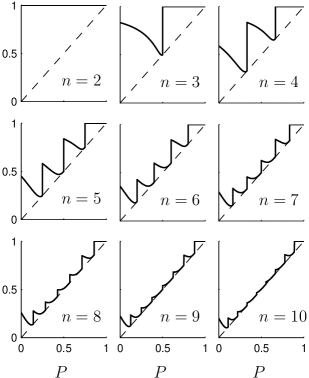
Figure 1: The payoff at equilibrium as a function of $P$ (thick line), for $T=1.2$ and group size $n\in\{2,\dots,10\}$. Also shown is the payoff $P$ (dashed line) for a population of pure all-defect. (Adapted from [20].)

The number of terms in direct evaluation of the expected fitness from (3) grows very rapidly with $n$. Hence, in order to simulate the evolutionary dynamics (2) for general population compositions, it is necessary to have an efficient method for evaluating the expected fitness of each strategy. Using the probability $P^{l}_{i}$ that the number of cooperating players equals $i$, in a group with one player using strategy $s_{l}$ and the $n-1$ other players chosen randomly from the population, we may express the expected fitness $f_{l}$ as

$$f_{l} = \sum_{i=0}^{l}P^{l}_{i}\,V\!(\text{D}|i)+\sum_{i=l+1}^{n}P^{l}_{i}\,V\!(\text{C}|i-1),$$ (6)

since strategy $s_{l}$ cooperates if $i>l$. Thus, efficient calculation of the $P^{l}_{i}$ allows for the study of the evolutionary dynamics in groups of more than a few players. Since $P^{l}_{i}$ only depends on the distribution of trigger levels in the population, this method may be applied for any payoff functions $V\!(\text{C}|i)$ and $V\!(\text{D}|i)$. In the previous paper [20] we derived the following formula for $P^{l}_{i}$:

$$P^{l}_{i} = \left\{\begin{array}[]{ll}0&\text{ whenever }i=l,\\ D^{l,0}_{n-1}&\text{ when }i=0,\\ \left(x_{0}+\ldots+x_{n-1}\right)^{n-1}&\text{ when }i=n,\\ \binom{n-1}{i-\mathbf{1}_{(l<i)}}\ \left(x_{0}+\ldots+x_{i-1}\right)^{i-\mathbf{1}_{(l<i)}}D^{l,i}_{n-1-i+\mathbf{1}_{(l\,<\,i)}}&\text{ otherwise, }\end{array}\right.$$ (11)

where $\mathbf{1}_{(l\,<\,i)}$ is one if $l<i$ and zero otherwise, and $D^{l,i}_{m}$ is given by the recursive formula

$$D^{l,i}_{m} = \left\{\begin{array}[]{ll}x_{n}^{m}&\text{ when }i=n-1\\ \sum\limits_{j=0}^{M}\binom{m}{j}\,x_{i+1}^{j}\,D^{l,i+1}_{m-j}&\text{ otherwise}\end{array}\right.$$ (14)

where $M=m+i+2-\mathbf{1}_{(l\,<\,i)}-n$. Note that whenever $l<i$ and $l^{\prime}<i$, $P^{l}_{i}=P^{l^{\prime}}_{i}$, so if $l<i$ then $P^{l}_{i}=P^{0}_{i}$. Using tables to store evaluated values of $D^{l,i}_{m}$, it is possible to evaluate the values of $P^{l}_{i}$ for all $l$ and $i$ in $\sim n^{4}$ operations.

4 Selection and mutation processes in finite populations

In [20] we introduced a simple model for incorporating mutations as an explicit part of the evolutionary dynamics. The population is subject to selection as in (2). In addition, a number $\mathcal{M}_{l\rightarrow j}$ of individuals per generation switch from strategy $s_{l}$ to strategy $s_{j}$ due to mutations. The mutations are assumed to be generated by uncorrelated stochastic events, e.g. by a Poisson process, in the process of reproduction. The evolutionary dynamics then takes the form

$$x^{\prime}_{i} = x_{i}+\delta\left(\frac{f_{i}}{\bar{f}}-1\right)x_{i}+\frac{1}{N}\sum_{j=0}^{n}(\mathcal{M}_{j\rightarrow i}-\mathcal{M}_{i\rightarrow j}).$$ (15)

In a single generation, each player with strategy $s_{i}$ has an expected number $\delta f_{i}x_{i}/\bar{f}$ of offspring surviving to reproductive age. Mutations occur independently in the creation of each offspring, with a probability of $\mu\ll 1$ per offspring per generation, and the strategy of the mutated offspring is chosen randomly among the $n+1$ strategies, with equal probability. Since the population size is assumed to be large, we approximate the number $\mathcal{M}_{i\rightarrow j}$ of mutated offspring with its expected value, $\mathcal{M}_{i\rightarrow j}\approx\mu\delta Nf_{i}x_{i}/[(n+1)\bar{f}]$. Inserting this approximation into (15), we obtain the following expression for the evolutionary dynamics:

$$x^{\prime}_{i} = x_{i}+\delta\left(\frac{f_{i}}{\bar{f}}-1\right)x_{i}+\delta\,\mu\left(\frac{1}{n+1}-\frac{f_{i}}{\bar{f}}\,x_{i}\right).$$ (16)

For some values of the payoff parameters, the strength of selection is so small compared to the flow mutants that the population does not converge to the evolutionary stable composition of strategies in the population. This is illustrated in Fig. 2a, where we show the asymptotic time-averaged average fitness in the population, for case of infrequent mutations [22] and for (16). For some values of $P$ the difference is clear; in this case, the dynamics either converge to a limit cycle (illustrated in Fig. 2b), or to a fixed point where three or more strategies coexist at significant levels.

\psfrag{x1}[t]{$P$}\psfrag{y1}{$\bar{f}$}\psfrag{atext2}{}\psfrag{n = 6}{\small$n=6$}\includegraphics[clip,height=142.26378pt]{avg_payoff.eps} a                                                                         \psfrag{x1}[t]{$P$}\psfrag{y1}{$\bar{f}$}\psfrag{atext2}{}\psfrag{n = 6}{\small$n=6$}\psfrag{xlabel}[t]{$\mu\,t$}\psfrag{ylabel}[b]{$x_{i}(t)$}\includegraphics[clip,height=136.5733pt]{n=6_oscillation_a.eps} b

Figure 2: a The time-averaged average payoff in the population as a function of $P$, for $n=6$, $T=1.6$, and $\mu=10^{-4}$. Also shown is the payoff in the limit of infinitesimal $\mu$ (thick line) and the payoff $P$ for a population of pure all-defect (dashed line). (Adapted from [20].) b The initial transient and two cycles of the attractor of the time evolution of the population for $P=0.33$ (Adapted from [20]). Within a cycle, strategy $s_{6}$ comes to dominate the population for a period of time. During the part of the cycle where strategy $s_{6}$ is prominent, the system approaches the population mixture which is evolutionarily stable when mutations are infrequent. For the value of $P$ used here, it corresponds to a mixture of strategies $s_{2}$ and $s_{6}$. For a period of time, this mixture of strategies dominates the population. After a while, however, $x_{5}$ starts to grow at the expense of $x_{6}$, and after a while there is another sharp transition where $x_{5}$ and $x_{2}$ grow and $x_{6}$ decay to very low levels.

In this article, we compare the results of the deterministic approximation (16) to explicit simulation of (15). It is natural to assume that in the stochastic model, the mutations in individuals with strategy $s_{i}$ occur according to a Poisson process with rate $\lambda_{i}=\mu\delta Nf_{i}x_{i}/[(n+1)\bar{f}]$. In each simulation step, the number of mutants of each strategy is drawn independently. For each mutation, the resulting strategy is drawn with uniform distribution and the fraction of the chosen strategy is incremented.

An additional source of stochastic fluctuations come from the selection of individuals from one generation to the next. The growth of the fraction $x_{i}$ of strategy $s_{i}$ in (2) may be viewed as a mean-field approximation of a more realistic stochastic growth process, in which the difference in fitness between two individuals is reflected in the probability distribution of their number of offspring. For simplicity, we model mutations as occurring separate from the selection process – in our computer simulations, we first generate the next generation according to the selection model, and then impose the effect of mutations as described above.

The selection process is as follows: in each generation, an individual with strategy $s$ produces a number of offspring in relation to the fitness of strategy $s$. It is assumed that the total number of offspring is more than enough to replace the parent generation. The fraction of the offspring with strategy $s_{i}$ is then

$$(1-\delta)x_{i}+\delta\,\frac{f_{i}}{\bar{f}}\,x_{i},$$ (17)

which we recognize as the fraction of $s_{i}$ in the next generation in the case of an infinite population size. Since the environment has a finite carrying capacity, we sample $N$ individuals uniformly from the offspring of the parent generation. Hence, the joint distribution of the number $k_{i}$ of players with strategy $s_{i}$ in the next generation is multinomial:

$$f(k_{0},\dots,k_{n}) = \frac{N!}{\prod_{i=0}^{n}k_{i}!}\,\prod_{i=0}^{n}\left[(1-\delta)x_{i}+\delta\,\frac{f_{i}}{\bar{f}}\,x_{i}\right]^{k_{i}},$$ (18)

provided the constraint $\sum_{i=0}^{n}k_{i}=N$ is fulfilled. In the limit of $N\rightarrow\infty$, the variance of $x^{\prime}_{i}=k_{i}/N$ vanishes, and the dynamics becomes deterministic, as expected.

The selection process can be approximated, for large populations, with a diffusion process: to each fraction $x_{i}$ we add a normal distributed number $\xi_{i}$ with zero mean and a variance $\delta x_{i}(1-x_{i})/N$. We take the variables $\xi_{i}$ and $\xi_{j}$ to be uncorrelated, for all $i\neq j$. If a fraction $x_{i}$ becomes negative, it is set to zero. Finally, the fractions are normalised so that $\sum_{i=0}^{n}x_{i}=1$. This approximation does not exhibit the correct correlations in the fluctuations of the $x_{i}$, but the magnitude of the fluctuations are approximately correct. Since the magnitude of the perturbations are small, however, correlations and higher-order cross-terms may be neglected.

5 Results

In Fig. 3 we illustrate the effect of random mutations and the finite population size on the evolution of the frequencies of the strategies, for a specific choice of the parameters. The effect is similar for other parameters; for parameter values where the deterministic approximation (16) converges to a fixed point (c.f. Fig. 2a), introducing a finite (large) population size does not change the qualitative properties of the long-term evolutionary dynamics, although the variance of the fraction of each strategy is increasing with decreasing population size.

\psfrag{t}{}\psfrag{xi}[t]{Fraction $x_{i}$}\includegraphics[clip]{mut_P=0.33_N=1e4.eps}	a                                                                 \psfrag{xi}{}\psfrag{t}{}\includegraphics[clip]{evol_P=0.33_N=1e8.eps} b
\psfrag{xi}[t]{Fraction $x_{i}$}\psfrag{t}[t]{$\mu t$}\includegraphics[clip]{evol_P=0.33_N=1e6.eps}	c                                                                 \psfrag{xi}{}\psfrag{t}[t]{$\mu t$}\includegraphics[clip]{evol_P=0.33_N=1e4.eps} d

Figure 3: Illustration of the effect of stochastic mutations and a finite population size on the evolution of strategies. The parameters are: $T=1.6$, $P=0.33$, $\mu=10^{-4}$ and the groups size $n=6$. The lines are: $s_{0}$ (blue), $s_{1}$ (green), $s_{2}$ (red), $s_{3}$ (cyan), $s_{4}$ (magenta), $s_{5}$ (yellow), and $s_{6}$ (black). In panel a we show the time evolution of a population with stochastic mutations but ignoring the effect of finite population size in the selection (population size $N=10^{4}$). In panels b, c, and d, both explicit mutation and selection is present. The effective population size $N$ takes the value $10^{8}$, $10^{6}$, and $10^{4}$, respectively.

We now focus on the fate of the limit cycles that are the most striking feature in the deviations of (16) from the evolutionary dynamics in the limit of infinitesimal mutation rate. The simulations show that, in the limit of very large populations, the analytical approximation (16) of how the flow of mutants alter the replicator dynamics is valid. As can be see from the smoothness of the curves in Fig. 3a, the main effect of the stochastic mutations compared to their deterministic counterpart is to add a little noise to the time evolution so that the curve fluctuates around the deterministic solution. Hence, unless the population size is small, the difference between the explicit mutations and the analytical approximation is negligible.

Fluctuations in the frequencies of strategies in the population due to random sampling in the selection play a very different role. Panels b–d in Fig. 3 illustrate the effect of these fluctuations for three values of the populations size. For very large populations ($N\sim 10^{8}$), the fluctuations do not alter the qualitative properties of the time evolution (panel b). However, for populations as large as $N=10^{6}$ individuals (panel c), we find that the fluctuations cause significant deviations from the deterministic model, while some qualitative aspects are the same: the time evolution still exhibit cycles, characterised by short periods where the composition is similar to that of the infrequent-mutation solution of Molander [22], interspersed with long periods of a high degree of cooperation and with a slow drift of strategies. The period of these cycles now fluctuate. When the population size is decreased to $N=10^{4}$, the cycles are no longer stable. The population now switches between irregular cyclic behaviour and more stable configurations in which three or more strategies co-exist. Preliminary investigations indicate that these configuration may have a stable counterpart in the deterministic approximation; it is not yet clear, however, if this he case for all parameter values.

6 Discussion and conclusions

The main purpose of this article (and also of the previous article [20]) is to better understand how more realistic models of the evolution of a population affects the evolution of the frequencies of strategies in the population. In the present article we have confirmed that – when the population size is large and the mutation rate is small – the deterministic approximation (16) provides an accurate description of the evolutionary dynamics. We have also shown that taking the fluctuations in the selection process into account may lead to different compositions of the strategies in the population than expected from the earlier analysis.

The fluctuations in the selection of individuals show a much stronger effect on the evolutionary dynamics than does the fluctuations from the mutation process. A large part of this difference can be understood from the magnitudes of these fluctuations, as characterized by their variances: in the mutation process, the variance contributed per time step is of order $[\delta\mu x_{i}/(n+1)]N^{-1}$, whereas in the selection process the variance is $\delta x_{i}(1-x_{i})N^{-1}$. When the mutation rate is small, and $x_{i}$ is not very close to one, $\mu/(n+1)\ll 1-x_{i}$. For instance, when $\mu=10^{-4}$, $N=10^{4}$, and $n=6$, as in Fig. 3a, the typical fluctuations due to mutations are of the same order as the fluctuations from the selection process in population with $N\sim 10^{8}$ individuals. This explains the good qualitative agreement between panels a and b in Fig. 3.

It remains to explain what causes the evolutionary dynamics to switch from the limit cycle to coexistence of three strategies in Fig. 3d. A hypothesis is that, apart from the limit cycle, there are stable fixed points with a small basin of attraction when the population evolves under (16); the fluctuations in the selection process may then cause a transition from one mode to the other and back. In this case we expect that the transitions between these modes occur, approximately, according to a Poisson process. The number of such fixed points, and to which extent the proposed mechanism can explain the observed dynamics, remains to be investigated.

References

- [1] G. Hardin. The tragedy of the commons. Science, 162:1243–1248, 1968.
- [2] J. Maynard Smith. Evolution and the Theory of Games. Cambridge University Press, Cambridge, 1982.
- [3] R. Sugden. The Economics of Rights, Co-operation and Welfare. Basil Blackwell, Oxford, 1986.
- [4] M. M. Flood. Some experimental games. Management Science, 5(1):5–26, 1958. First published in Report RM-789-1, The Rand Corporation, Santa Monica, CA, 1952.
- [5] A. Rapoport and A. M. Chammah. Prisoner’s Dilemma. University of Michigan Press, Ann Arbor, 1965.
- [6] R. Axelrod and D. H. Hamilton. The evolution of cooperation. Science, 211:1390 – 1396, 1981.
- [7] P. Molander. The optimal level of generosity in a selfish, uncertain environment. J. Conflict Resolution, 29:611 – 618, 1985.
- [8] R. Axelrod. The evolution of strategies in the iterated prisoner’s dilemma. In Davis L, editor, Genetic Algorithms and Simulated Annealing, pages 32 – 41. Morgan Kaufmann, Los Altos, CA, 1987.
- [9] J. H. Miller. The coevolution of automata in the repeated Prisoner’s Dilemma. J. Econ. Behav. Organ., 29(1):87–112, 1996. Appeared 1989 as a Santa Fe Institute working paper.
- [10] K. Lindgren. Evolutionary phenomena in simple dynamics. In Langton, C. G. et al, editor, Artificial Life II, pages 295 – 311. Addison-Wesley, Redwood City, CA, 1992.
- [11] M. A. Nowak and K. Sigmund. Tit for tat in heterogenous populations. Nature, 359:250–253, 1992.
- [12] K. Matsuo. Ecological characteristics of strategic groups in ’dilemmatic world’. In IEEE International Conference on Systems and Cybernetics, pages 1071 – 1075, 1985.
- [13] N. Adatchi and K. Matsuo. Ecological dynamics under different selection rules in distributed and iterated prisoner’s dilemma games. In Parallel Problem Solving From Nature, volume 496 of Lecture Notes in Computer Science, pages 388–394. Springer, Berlin, 1991.
- [14] N. Adatchi and K. Matsuo. Ecological dynamics of strategic species in game world. Fujitsu Sci. Tech. J., 195:543–558, 1992.
- [15] P. Albin. Approximations of cooperative equilibria in multi-person Prisoner’s Dilemma played by cellular automata. Math. Soc. Sci., 24:293–319, 1992.
- [16] C. Hauert and H. G. Schuster. Effects of increasing the number of players and memory size in the iterated Prisoner’s Dilemma, a numerical approach. Proc. R. Soc. B London, 264:513–519, 1997.
- [17] V. Akimov and M. Soutchanski. Automata simulation of -person social dilemma games. J. Conflict Resolution, 38:138–148, 1997.
- [18] M. Matsushima and T. Ikegami. Evolution of strategies in the three-person iterated prisoner’s dilemma game. J. Theor. Biol., 195:53–67, 1998.
- [19] K. Lindgren and J. Johansson. Coevolution of strategies in -person Prisoner’s Dilemma. In J. Crutchfield and P. Schuster, editors, Evolutionary Dynamics - Exploring the Interplay of Selection, Neutrality, Accident, and Function. Addison-Wesley, 2001.
- [20] A. Eriksson and K. Lindgren. Cooperation driven by mutations in multi-person prisoner’s dilemma. J. Theor. Biol., 232(3):399–409, 2005.
- [21] R. Boyd and P. Richerson. The evolution of reciprocity in sizable groups. J. Theor. Biol., 132:337–356, 1988.
- [22] P. Molander. The prevalence of free riding. J. Conflict Resolution, 36:756–771, 1992.
- [23] T. C. Schelling. Micromotives and Macrobehaviour. Norton, New York, 1978.