Transient Resetting: A Novel Mechanism for Synchrony and Its Biological Examples

Abstract

The study of synchronization in biological systems is essential for the understanding of the rhythmic phenomena of living organisms at both molecular and cellular levels. In this paper, by using simple dynamical systems theory, we present a novel mechanism, named transient resetting, for the synchronization of uncoupled biological oscillators with stimuli. This mechanism not only can unify and extend many existing results on (deterministic and stochastic) stimulus-induced synchrony, but also may actually play an important role in biological rhythms. We argue that transient resetting is a possible mechanism for the synchronization in many biological organisms, which might also be further used in medical therapy of rhythmic disorders. Examples on the synchronization of neural and circadian oscillators are presented to verify our hypothesis.

Synopsis:

Synchronization of dynamical systems is a dynamical process wherein two (or many) systems (either identical or nonidentical) adjust a given property of their motions to a common behavior due to coupling or forcing. Synchronization has attracted much attentions of physicists, biologists, applied mathematicians, and engineers for many years. In this paper, we present a very simple, but generally applicable mechanism, named transient resetting, for stimulus-induced synchronization of dynamic systems. The mechanism is applicable not only to periodic oscillators but also to chaotic ones, and not only to continuous time systems but also to discrete time ones. Biological systems are dynamic, and the synchronization in biological systems is essential, for example, for the understanding of their rhythmic phenomena and information processing. In this paper, we study several possible applications in the biological context after presenting the novel mechanism. We also show that transient resetting might also be used in medical therapy of rhythmic disorders. Beneficial roles of noise in biological systems have been extensively studied in recent years. Our mechanism can also be seen as an explanation of the beneficial roles of noise on the synchronization in biological systems, though the stimulus is not necessarily required to be noisy in our mechanism.

Introduction

Life is rhythmic. Winfree showed us a shocking discovery that a stimulus of appropriate timing and duration can reset (stop) the biological rhythm by driving the clock to a “phase singularity”, at which all the phases of the cycle converge and the rhythm’s amplitude vanishes. He theoretically predicted this in the late 1960s, and then confirmed it experimentally for the circadian rhythm of hatching in populations of fruitflies. Subsequent studies have shown that mild perturbations can also quench other kinds of biological oscillations, for example, the breathing rhythms and neural pacemaker oscillations [1, 2]. Such findings may ultimately have medical relevance to disorders involving the loss of a biological rhythm, such as sudden infant death or certain types of cardiac arrhythmias [3]. In [4], Tass studied phase resetting by using methods and strategies from synergetics. In [5], Leloup and Goldbeter presented an explanation for this kind of long-term suppression of circadian rhythms by the coexistence of a stable periodic oscillation and a stable steady state in the bifurcation diagram.

On the other hand, synchronization is essential for biological rhythms and information processing in biological organisms. So far, many researchers have studied the synchronization in biological systems experimentally, numerically and theoretically. In this paper, by using simple dynamical systems theory, we show that transient resetting, which concept will be clarified later, can play a constructive role for biological synchrony. We argue that transient resetting is a possible mechanism for synchrony generally used in many biological organisms, which might also be further used in medical therapy of rhythmic disorders. Winfree’s results showed the destructive aspect of the resetting, while we show its constructive aspect in this paper. Although we concentrate mainly on biological systems here, the novel mechanism presented in this paper is applicable to general oscillators, so in the following, we first present it as a general mechanism for synchrony and then discuss its possible applications to biological rhythms.

Results

Basic mechanism

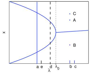
Figure 1: A schematic bifurcation diagram with a normal (supercritical) Hopf bifurcation for illustrating the transient resetting mechanism.

Let’s assume that an oscillator has a bifurcation diagram like that shown in Fig. 1 with a normal (supercritical) Hopf bifurcation [6], in which the bifurcation parameter $\lambda$ is the above mentioned “stimulus” and the curves with $\lambda<\lambda_{0}$ show the maximum and minimum values of the stable limit cycle. When the stimulus is a constant less than the critical value (bifurcation point) $\lambda_{0}$, the system has a stable rhythm (periodic oscillation); when the stimulus $\lambda>\lambda_{0}$, the system has a stable equilibrium state, which is shown by the curve with $\lambda>\lambda_{0}$. Undoubtedly, many oscillators have this kind of bifurcation structure. Assume that a population of (identical) oscillators operate in stable periodic states with $\lambda=a$. To clarify the essential role of transient resetting, we don’t consider coupling among oscillators in this paper. For oscillators without coupling, the situation for studying the synchronization of two oscillators is the same as that for a population of oscillators, so in the following, we always consider two oscillators. Let’s also assume that there are some common fluctuations, e.g. periodic fluctuations or random noise, that can perturb the parameter $\lambda$ from $a$ to the right-hand side of $\lambda_{0}$, say to $\lambda=b$ in Fig. 1, from time to time. When the duration for the oscillators staying at the right-hand side of $\lambda_{0}$ is long enough, the two oscillators will all converge to the steady state, which is a rhythm-vanishing phenomenon. Next, let’s examine what will happen when the parameter $\lambda$ visit the value $\lambda=b$ for a short duration. If the states of the two oscillators are at points $A$ and $B$ respectively, the two oscillators will have the tendency to converge to their common steady state when the parameter $\lambda$ visits the value $\lambda=b$, which means that the states of the two oscillators will have the tendency to become closer. If the states of the two oscillators are at the points $A$ and $C$ respectively, the two oscillators will also have the tendency to converge to their common steady state when the parameter $\lambda$ visits the value $\lambda=b$. From conventional linear stability analysis, we know that the velocity for converging to the steady state at point $C$ is higher than that at point $A$, so the two oscillators will also have the tendency to become closer. Thus, by short-time visiting the right-hand side of $\lambda_{0}$, the states of the two oscillators always become closer, which is helpful for the genesis of synchronization between the oscillators. Here the states of the oscillators are not really reset to the steady state, but they have the tendency (for a short time) to be reset to the steady state, which is the reason we call it transient resetting.

From the above analysis, it is easy to know that the bifurcation is not necessarily required to be a supercritical Hopf bifurcation. We only need that the oscillator operates, in most times, in an oscillatory state, and can from time to time visit a steady state in the parameter space (the solutions are all unique in these two states). Even if there are other bifurcations between these two states ($\lambda=a$ and $\lambda=b$), say a subcritical Hopf bifurcation with coexistence of a stable limit cycle and a stable equilibrium state between the dashed and the dotted vertical lines in Fig. 1, the above argument can also hold. Moreover, since oscillators are usually nonidentical in real systems, there are some mismatches between the oscillators. If the mismatches are not so large, however the oscillators can also be synchronized (although not perfectly) by transient resetting. For example, we assume that the mismatch can be reflected in the parameter $\lambda$, and assume that the two oscillators operate with parameters $\lambda=a$ and $\lambda=e$ respectively, and by a common perturbation, the parameters of the two oscillators visit $\lambda=b$ and $\lambda=c$ respectively in Fig. 1. If the mismatch between the systems is not so large, the distance between the steady states with $\lambda=b$ and $\lambda=c$ is most likely small as well. The two oscillators have the tendency to be contracted to the two steady states respectively, which mean that roughly they are becoming closer since the two steady states are close. In transient resetting, we don’t care what the stimulus is. It can be of any kinds, say periodic, random, impulsive, or even chaotic stimuli, thus the transient resetting can unify many existing results on stimulus-induced synchrony.

Next, we present several examples on biological rhythms to show the effectiveness of the transient resetting and its biological plausibility as a mechanism for biological synchrony.

Reliability of neural spike timing

A remarkable reliability of spike timing of neocortical neurons was experimentally observed in [7]. In the experiments, rat neocortical neurons are stimulated by input currents. When the input is a constant current, a neuron generates different spike trains in repeated experiments with the same input. It is evident that the constant input when viewed as a bifurcation parameter has moved the neuron dynamics from a steady state into a repetitive spiking regime. It is shown that when a Gaussian white noise is added to the constant current, the neuron generates almost the same spike trains in repeated experiments. From the viewpoint of synchronization, the repeated firing patterns imply that a common synaptic current can induce almost complete synchronization in a population of uncoupled identical neurons with different initial conditions. This kind of synchronization may have great significance in information transmission and processing in the brain (see, e.g. [8, 9, 10, 11, 12]).

We simulate the above mentioned behavior by using the well-known Hodgkin-Huxley (HH) neuron model, which is described by the following set of equations [13]:

$$\begin{array}[]{rl}C_{m}\dot{u}(t)=&G_{Na}m^{3}h(E_{N}a-u)+G_{K}n^{4}(E_{K}-u)\\ &+G_{m}(V_{\mbox{rest}}-u)+I_{0}+I(t),\\ \dot{m}(t)=&\alpha_{m}(u)(1-m)-\beta_{m}m,\\ \dot{h}(t)=&\alpha_{h}(u)(1-h)-\beta_{h}h,\\ \dot{n}(t)=&\alpha_{n}(u)(1-n)-\beta_{n}n,\end{array}$$ (1)

where $u(t)$ represents the membrane potential of the neural oscillator, $m(t)$ and $h(t)$ the activation and the inactivation of its sodium channel, $n(t)$ the activation of the potassium channel, $I_{0}$ the constant input current, and $I(t)$ the time-varying forcing. $\alpha_{x}$ and $\beta_{x}$ ($x=m,h,n$) are rate functions that are given by the following equations:

$$\begin{array}[]{c}\alpha_{m}(u)=\frac{0.1(25-u)}{\mbox{exp}\left(\frac{25-u}{10}\right)-1},\,\beta_{m}(u)=4\mbox{exp}\left(-\frac{u}{18}\right),\\ \alpha_{h}(u)=0.07\mbox{exp}\left(-\frac{u}{20}\right),\,\beta_{h}(u)=\frac{1}{\mbox{exp}\left(\frac{30-u}{10}\right)+1},\\ \alpha_{n}(u)=\frac{0.01(10-u)}{\mbox{exp}\left(\frac{10-u}{10}\right)-1},\,\beta_{n}(u)=0.125\mbox{exp}\left(-\frac{u}{80}\right).\end{array}$$

The parameters are set as the standard values [13], i.e. $G_{Na}$=120 mS/cm², $E_{Na}$=115 mV, $G_{K}$=36 mS/cm², $G_{m}$=0.3 mS/cm², $V_{\mbox{rest}}$=10.6 mV, and $C_{m}$=1 $\mu$F/cm². We always set the input $I_{0}+I(t)$ being zero for $t<0$. When $I(t)=0$, if the value $I_{0}$ is larger than a critical value $I_{0}^{c}\thickapprox 6$ $\mu$A/cm², the neuron has regular spiking; otherwise, the neuron is in the steady resting state. Thus, the bifurcation direction of HH neuron is opposite to that shown in Fig. 1 and the type of Hopf bifurcation is subcritical rather than supercritical. We fix the input constant $I_{0}=10$, such that when $I(t)=0\,(t>0)$, this model exhibits a stable periodic oscillation.

To simulate the experimental results in [7], we let $I(t)=D\xi(t)$ in the HH model, where $D$ is a positive constant, and $\xi(t)$ is a normal Gaussian white noise process with mean zero and standard deviation one. We numerically calculate the stochastic neuron model by using the Euler-Maruyama scheme [14] with time step $h=0.01$. When $D=2$, the two HH neural oscillators can achieve complete synchronization as shown in Fig. 2 (a). One may ask whether it is really the “noisy” property of $I(t)$ that synchronizes the oscillators. We show here that this behavior can be interpreted by the transient resetting mechanism. In fact, when $I(t)$ is a random noise, it will make the total input $I_{0}+I(t)$ visit the parameter region that is smaller than the critical value $I_{0}^{c}\thickapprox 6$ from time to time, so that the transient resetting mechanism can take effect. In the experiments, the total input is indeed below the critical value in some time durations, which implies that our argument is biological plausible. The experimental (and simulation) results show that the larger the noise intensity (to some extent), the higher the reliability and precision of the spike timing, which can also be interpreted by the transient resetting mechanism. In fact, when the noise intensity is larger, the total input will spend more time to be below $I_{0}^{c}$, such that the two trajectories will have more opportunities to be contracted together. Due to the random property of the input, when the input value is above $I_{0}^{c}$, the effects of the noise for converging and diverging the two trajectories are roughly balanced, thus, the longer the duration of the input value being below $I_{0}^{c}$, the closer the two trajectories and the faster the convergence should be. To further verify the above argument that it is not the “noisy” property of the input that synchronizes the oscillators, we perform another simulation, in which the fluctuation is a square wave with amplitude of 4.5 and period of 20 ms, that is, the total input switches between 10 (above $I_{0}^{c}$) and 5.5 (a little below $I_{0}^{c}$) every 10 ms. In Fig. 2 (b), we show the simulation result, in which the square wave is added at $t=80$. We see that the two neural oscillators are synchronized rapidly, though the input is a regular square wave.

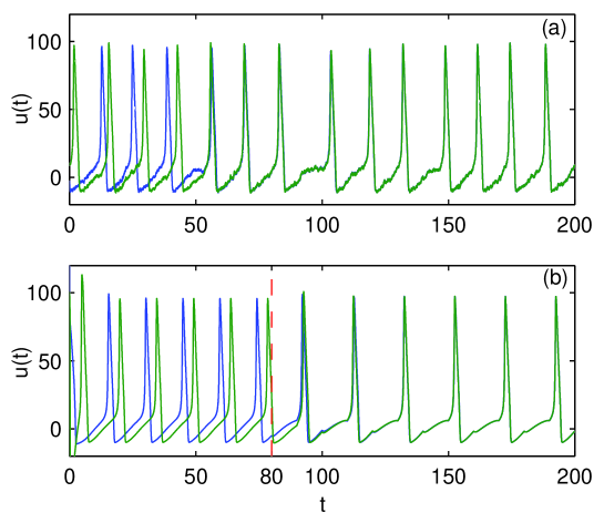
Figure 2: Synchronization of two Hodgkin-Huxley neural oscillators: (a) driven by common Gaussian white noise; and (b) driven by a common square wave.

Next, we numerically study the relationship between the time rate that the stimulus of the HH neuron model spends in the steady state regime (defined as the duty) and the time required to achieve synchronization. For the convenience of measuring the duty, we use square waves as the stimulus in the simulations. In the following simulation, the period of the square wave is 20ms, the time window when the stimulus is in the steady state parameter regime is randomly chosen in each cycle, and all the other parameters are the same as those in the above simulation. In Fig. 3, we plot the relationship between the duty and the time required to achieve synchronization as the duty increases from 0.1 to 0.4 with step 0.05, in which the data are obtained by averaging the results in 20 independent runs. Fig. 3 shows that the time required to achieve synchronization decreases as the duty increases. This quantitative result again confirms our above argument and provides a numerical evidence that the proposed mechanism can account for the observed synchrony.

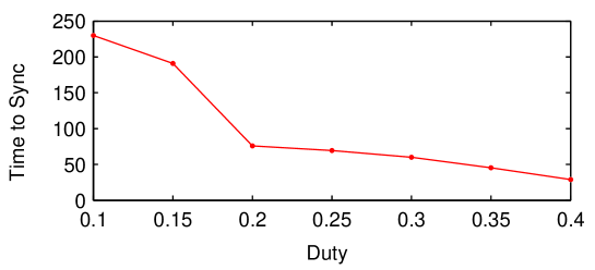
Figure 3: The relationship between the duty and the time required to achieve synchronization in the HH neuron model.

Biological oscillators are usually nonidentical in real systems, and there are some mismatches between the oscillators. As we mentioned in the Basic Mechanism section, if the mismatches are not so large, the oscillators can also be synchronized (although not perfectly) by the transient resetting. We next numerically study the relationship between the parameter mismatch and the synchronization error, that is, the robustness of the mechanism, in the HH systems. In this simulation, we consider the mismatch on $I_{0}$ in Eq. (1), namely in one of the two neural oscillators, the constant input is $I_{0}-\Delta I$, and in the other one, it is $I_{0}$. As we know, the input value $I$ has explicit effect on the spiking frequency of the HH neuron model. We also use square wave in this simulation, and the period and the duty are 10 and 0.3, respectively. The synchronization error is defined as $q=<|X_{1}(t)-X_{2}(t)|>$, where $X_{1},X_{2}$ are the state vectors of the two neural oscillators, that is $X_{i}(t)=[u_{i}(t),m_{i}(t),h_{i}(t),n_{i}(t)]^{T},i=1,2$, and $<\cdot>$ is the average over time after discarding the initial phase of the simulation for 100ms. In Fig. 4(a), we plot the relationship between $\Delta I$ and $q$, in which each value of $q$ is also obtained by averaging the results in 20 independent runs and the error bars denote the standard deviations. Fig. 4(a) show that the synchronization error $q$ increases with the increasing of $\Delta I$, and when $\Delta I$ is not so large, the systems can also achieve synchronization with a small synchronization error $q$. In Fig. 4(b), we plot a typical simulation result with $\Delta I=0.5$, and the $q$ value between 100ms and 200ms in this simulation is $q=3.8667$. Fig. 4(b) demonstrates that the transient resetting mechanism can indeed make the two nonidentical neural oscillators synchrony, though the synchrony is not perfect. When the mismatch becomes large, the systems may intermittently lose synchrony, but shortly after that the systems can be attracted back to synchrony again by the mechanism. When the mismatch becomes much larger, the systems cannot maintain the synchronous state, though the mechanism still have the tendency to draw the systems together. In biological systems, the oscillators, though not perfectly identical, can usually be similar and the mismatch may not be so large. Thus the presented mechanism is robust in such cases. Moreover, the synchronization in biological systems may not be required to be perfect for emergence of functions.

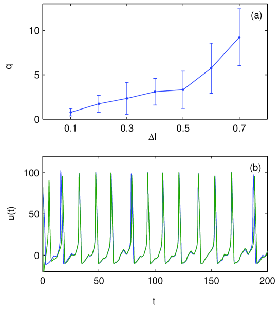
Figure 4: Robustness of the mechanism with parameter mismatch on $I_{0}$: (a) The relationship between the parameter mismatch $\Delta I$ and the synchronization error $q$ in the HH neuron model. (b) A typical numerical result of the systems with $\Delta I=0.5$.

It should be noted that when the mismatches exist in other parameters, except the input, we can also obtain similar results. For example, in another simulation, we consider a mismatch on the parameter $G_{m}$, that is the parameter is $G_{m}+\Delta G_{m}$ in one oscillator, and it is $G_{m}$ in the other oscillator. The simulation method are the same as above. In Fig. 5(a), we show the relationship between $\Delta G_{m}$ and $q$ as $\Delta G_{m}$ increases from 0.02 to 0.1 with step 0.02. In Fig. 5(b), we plot a typical numerical result with $\Delta G_{m}=0.06$, and the $q$ value between 100ms and 200ms in this simulation is $q=2.1492$. From this figure, we can get the same conclusion as that in the above example.

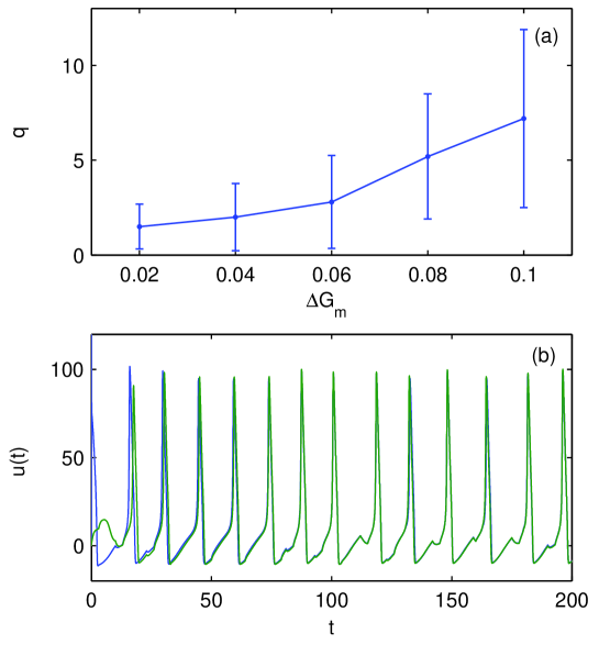
Figure 5: Robustness of the mechanism with parameter mismatch on $G_{m}$: (a) The relationship between the parameter mismatch $\Delta G_{m}$ and the synchronization error $q$ in the HH neuron model. (b) A typical numerical result of the systems with $\Delta G_{m}=0.06$.

It should also be noted that this transient resetting is effective for both class I and class II neuron [13]. Further, the Hopf bifurcation of class II neurons can be either subcritical like the HH model or supercritical associated with the canard phenomenon [15].

Circadian oscillators

In circadian systems, the light-dark cycle is the dominant environmental synchronizer used to entrain the oscillators to the geophysical 24-h day. In the following, we show that the light-dark cycle as a synchronizer can also be interpreted by the transient resetting mechanism. By our argument on transient resetting, if the circadian clock has a bifurcation diagram similar to Fig. 1 with a light-affected parameter as the bifurcation parameter, and if the oscillators operate in the oscillatory parameter region (say with $\lambda=a$ in Fig. 1) in the dark duration, and in the steady state parameter region (say with $\lambda=b$ in Fig. 1) in the light duration, the oscillators may be automatically synchronized. For example, in the Leloup-Goldbeter model of the Drosophila [16], the light-dark cycle affects the degradation of the concentration of TIM protein. In their parameter setting (which is biologically plausible), under a continuous light condition, the model is in the steady state parameter region. Then, according to the transient resetting mechanism, the uncoupled oscillators can be synchronized automatically, which is verified by our numerical simulations (data not shown).

In theoretical studies of circadian clocks, the light-dark cycle is usually represented by a square wave, but in fact, even with continuous light, the light intensity includes fluctuations (light noise). Next, we study the effect of light noise on the synchronization of circadian oscillators. We consider the Goldbeter circadian clock model of the Drosophila [17] as an example, which is described as follows:

$$\begin{array}[]{l}\frac{dM}{dt}=v_{s}\frac{K_{I}^{n}}{K_{I}^{n}+P_{N}^{n}}-v_{m}\frac{M}{K_{m}+M},\\ \frac{dP_{0}}{dt}=k_{s}M-V_{1}\frac{P_{0}}{K_{1}+P_{0}}+V_{2}\frac{P_{1}}{K_{2}+P_{1}},\\ \frac{dP_{1}}{dt}=V_{1}\frac{P_{0}}{K_{1}+P_{0}}-V_{2}\frac{P_{1}}{K_{2}+P_{1}}-V_{3}\frac{P_{1}}{K_{3}+P_{1}}+V_{4}\frac{P_{2}}{K_{4}+P_{2}},\\ \frac{dP_{2}}{dt}=V_{3}\frac{P_{1}}{K_{3}+P_{1}}-V_{4}\frac{P_{2}}{K_{4}+P_{2}}-k_{1}P_{2}+k_{2}P_{N}-v_{d}\frac{P_{2}}{K_{d}+P_{2}},\\ \frac{dP_{N}}{dt}=k_{1}P_{2}-k_{2}P_{N},\end{array}$$ (2)

where the parameter values are $v_{s}$=0.76 $\mu$Mh^-1, $v_{m}$=0.75 $\mu$Mh^-1, $K_{m}=0.5$ $\mu$M, $k_{s}$=0.38 h^-1, $v_{d}$=1 $\mu$Mh^-1, $k_{1}$=1.9h^-1, $k_{2}$=1.3h^-1, $K_{I}=1$ $\mu$M, $K_{d}$=0.2 $\mu$M, $n$=4, $K_{1}=K_{2}=K_{3}=K_{4}=2$ $\mu$M, $V_{1}$=3.2 $\mu$Mh^-1, $V_{2}=1.58$ $\mu$Mh^-1, $V_{3}$=5 $\mu$Mh^-1, and $V_{4}$=2.5 $\mu$Mh^-1 (see [17] for more details about this model). In this model, light enhances the degradation of the PER protein by increasing the value of $v_{d}$. With these biologically plausible parameter values, the period of the circadian clock is about 24h. With the increasing of $v_{d}$, there is a Hopf bifurcation similar to that shown in Fig. 1, and the critical value of $v_{d}$ at the bifurcation point is about 1.6. To clarify the effect of light noise, we don’t consider the light-dark cycle in this simulation, that is $v_{d}=1$ is a constant (denoting the average light intensity) if there is no light fluctuations. In our simulation, we set $v_{d}=1+D\xi(t)$. When $D=0.15$, the simulation result is shown in Fig. 6(a), which shows that the two circadian oscillators achieve complete synchronization. This behavior can again be interpreted by the transient resetting mechanism. The interpretation is the same as that in the HH neural oscillator case.

In the above examples, we show separately the effects of the light-dark cycle and the light noise. The light-dark cycle itself may not be strong enough to reach the steady state parameter region in real biological circadian systems. For example, in Fig. 1, the light-dark cycle may make the bifurcation parameter switch between $a$ and $d$ in the dark and the light durations, respectively. In this case, a small light noise would drive the parameter $\lambda$ to the right hand side of $\lambda_{0}$ from time to time (in the light duration), which can be seen as the combination or synergetic effect of the light-dark cycle and the light noise. In other words, in biological circadian systems, it is likely that the light-dark cycle and the light noise cooperate to realize the transient resetting.

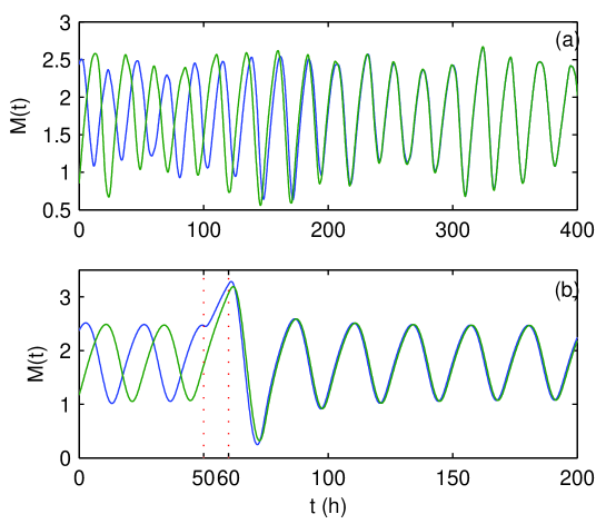
Figure 6: Synchronization of two Goldbeter circadian oscillators: (a) induced by common light noise; and (b) induced by a short duration of bright light.

The time required to achieve synchrony and the robustness of the mechanism in this system can also be studied similarly as in the HH model, although we omit the detailed results here.

Therapy

The transient resetting mechanism may have potential applications in the therapy of various rhythmic disorders. Our analysis implies that if we have some methods to control a biological rhythmic system to make it visit its steady state parameter region transiently, it may entrain the disordered rhythmic system to a synchronous state. For example, we use a stimulation bright light for 10 hrs with $v_{d}=1.7$ in $t\in[50,60]$, and $v_{d}=1$ in other time durations in the Goldbeter circadian oscillators. The simulation result is shown in Fig. 6 (b), which shows that the two oscillators are almost completely synchronized after the short duration of the bright light stimulation. The exposure to bright light also induces a several-hour delay shift of the circadian oscillators, which is consistent with the experimental results [18].

Except the above mentioned neural and circadian systems, the mitotic control system [19] may be another biological example that uses transient resetting mechanism to achieve synchrony.

Chaotic neuron model

In the above examples, we considered periodic oscillators, but the transient resetting, as a general mechanism for synchrony, can also be applied to chaotic systems. Clearly, the synchronization of chaotic systems is more difficult, because uncoupled chaotic oscillators, even with identical parameter values, will exponentially diverge due to the high sensitivity to perturbations. If the converging effect in steady state parameter region is larger than the diverging effect in chaotic parameter region, however the uncoupled chaotic systems may also be synchronized by the mechanism. Here, we consider a simple discrete-time chaotic neuron model described as follows [22]:

$$x(t+1)=kx(t)-\alpha f(x(t))+a+I(t)$$ (3)

where $f(x(t))=1/[1+\mbox{exp}(-x(t)/\epsilon)]$. This neuron model is a model of the chaotic responses electrophysiologically observed in squid giant axons [23]. When decreasing $a$ from a large to a small value, the system undergoes a period-doubling road to chaos. We set the parameters $k=0.7,\alpha=1.05,a=0.93$ and $\epsilon=0.02$, such that when $I(t)=0$ the model exhibits chaotic dynamics. When $I>0.11$, the neuron model is in a steady state. In this example, we let $I(t)=0.15\xi(t)$ with $\xi(t)$ as a normal Gaussian white noise process as defined before, such that the neuron model can switch between chaotic states and steady states. The numerical result in Fig. 7 indicates that the chaotic neurons can indeed be synchronized by common noise, which can also be interpreted by the transient resetting mechanism.

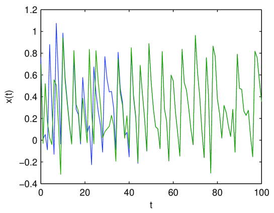
Figure 7: Synchronization of two chaotic neurons induced by common noise.

This example, though simple, shows that the transient resetting mechanism is applicable not only to periodic oscillators but also to chaotic systems, and not only to continuous time systems but also to discrete time systems. We can also see that, as we mentioned above, the bifurcation is not necessarily required to be a Hopf bifurcation.

Discussion

In literature, there exist some interesting results on noise-induced synchronization of oscillators, which can be classified into two classes: the noise depends or doesn’t depend on the states of the oscillators. In the case that that noise depends on the states of the oscillators (see, e.g. [20, 21]), the noise can, in fact, be seen as a kind of information exchange or coupling with fluctuant coupling strengths, and it is well known that coupling can induce synchronization, so it is not surprising that the noise can induce synchronization. In the case that noise doesn’t depend on the states, many existing results can be interpreted by the transient resetting proposed in this paper. Some studies also theoretically explained the mechanisms of periodic input forcing induced synchrony in literature. It should be noted that the fluctuations in the present mechanism of transient resetting are the parameters, not necessarily (but can be) the inputs. Synchronization induced by the fluctuations of some special parameters, for example time delay in delayed systems, can also be interpreted by the mechanism. Thus the transient resetting presented in this paper not only can unify and extend many existing results on various fluctuation induced synchrony, but also is very simple. It is reasonable to believe that life systems, after long time of evolution, use as simple as possible mechanisms to achieve complex functions.

It should also be noted, on the other hand, that although we have shown in this paper the transient resetting as a possible general mechanism for biological synchrony, we don’t exclude other possible mechanisms. Some systems driven by some specific inputs, which don’t satisfy the conditions shown in this paper, can also be synchronized. It should not be surprising that in biological systems, many mechanisms work together to jointly guarantee the robustness and precision of synchrony.

In summary, in this paper, by simple dynamical systems theory, we have presented a novel mechanism for synchrony based on the transient resetting, and we have shown that it could be a possible mechanism for biological synchrony, which can also potentially be used for medical therapy. In contrast with Winfree’s results, we have shown the constructive aspect of (transient) resetting here. In this paper, we are interested in the general qualitative mechanism, so in the simulations, we didn’t show many quantitative details for each specific example. In Fig. 1, we showed a 1-parameter bifurcation diagram. In some systems, there might be multiple parameters that affected by the fluctuations of stimuli. In that case, we can use a similar multi-parameter bifurcation diagram to understand the mechanism.

Materials and Methods

To simulate the stocahstic differential equaiton $\dot{x}(t)=f(x)+g(x)\xi(t)$, the Euler-Maruyama scheme is used in this paper. In this scheme, the numerical trajectory is generated by $x_{n+1}=x_{n}+hf(x_{n})+\sqrt{h}g(x_{n})\eta_{n}$, where $h$ is the time step and $\eta_{n}$ is a discrete time Gaussian white noise with $<\eta_{n}>=0$ and $<\eta_{n}\eta_{m}>=\delta_{nm}$. For more details, see e.g. [14].

References

- [1] Winfree AT (1970) Integrative view of resetting a circadian clock. J. Theor. Biol. 28: 327-374.
- [2] Winfree AT (2001) The Geometry of Biological Times (2nd Ed.). Springer-Verlag, New York.
- [3] Strogatz SH (2003) Obituary: Arthur T. Winfree. SIAM News 36: 1, available at http://www.siam.org/ siamnews/01-03/winfree.htm.
- [4] Tass PA (1999) Phase Resetting in Medicine and Biology: Stochastic Modelling and Data Analysis, Springer-Verlag, Berlin.
- [5] Leloup JC and Goldbeter A (2001) A molecular explanation for the long-term suppression of circadian rhythms by single light pulse. Am. J. Physiol.- Regul. Intergr. Compu. Physiol. 280: R1206-1212.
- [6] Guckenheimer J and Holmes P (1983) Nonlinear Oscillations, Dynamical Systems, and Bifurcations of Vector Fields. Springer-Verlag, New York.
- [7] Mainen ZF, Sejnowski TJ (1995) Reliability of spike timing in neocortical neurons. Science 268: 1503-1506.
- [8] de Oliveira SC, Thiele A, Hoffmann KP (1997) Synchronization of neuronal activity during stimulus expectation in a direction discrimination task. J. Neurosci. 17: 9248-9260.
- [9] Riehle A, Grun S, Diesmann M, Aertsen A (1997) Spike synchronization and rate modulation differentially involved in motor cortical function. Science 278: 1950-1953.
- [10] Steinmetz PN, Roy A, Fitzgerald PJ, Hsiao SS, Johnson KO, et al. (2000) Attention modulates synchronized neuronal firing in primate somatosensory cortex. Nature 404: 187-190.
- [11] Zhou C and Kurths J (2003) Noise-induced synchronization and coherence resonance of a Hodgkin-Huxley model of thermally sensitive neurons. Chaos 13: 401- 409.
- [12] Brette R, and Guigon E (2003) Reliability of spike timing is a general property of spiking model neurons. Neural Comput 15: 279-308.
- [13] Gerstner W, Kistler WM (2002) Spiking Neuron Models. Cambridge University Press.
- [14] Kloeden PE, Platen E and Schurz H (1994) Numerical solution of SDE through computer experiments. Springer-Verlag.
- [15] Diener M (1984) The canard unchained or how fast slow dynamical-systems bifurcate. Math. Intell. 6: 38-49.
- [16] Leloup JC, Gonze D, Goldbeter A (1999) Limit cycle models for circadian rhythms based on transcriptional regulation in Drosophila and Neurospora. J. Biol. Rhythms 14: 433-448.
- [17] Goldbeter A (1995) A model for circadian oscillations in the Drosophila period protein (PER). Proc. R. Soc. Lond. B 261: 319-324.
- [18] Czeisler CC, Allan JS, Strogatz SH, Ronda JM, Sanchez R, et al. (1986) Bright light resets the human circadian pacemaker independent of the timing of the sleep-wake cycle. Science 233: 667-671.
- [19] Closson TLL, Roussel MR (2000) Synchronization by irregular inactivation. Phys. Rev. Lett. 85: 3974-3977.
- [20] Chen L, Wang R, Zhou T, Aihara K (2005) Noise-induced cooperative behavior in a multicell system. Bioinfor. 22: 2722-2729.
- [21] Zhou T, Chen L, Aihara K (2005) Molecular communication through stochastic synchronization induced by extracellular fluctuations. Phys. Rev. Lett. 95: 178103.
- [22] Aihara K, Takabe T, and Toyoda M (1990) Chaotic neural networks. Phys. Lett. A 144: 333-340.
- [23] Matsumoto G, Aihara K, Hanyu Y, Takahashi N, Yoshizawa S, Nagumo J (1987) Chaos and phase locking in normal squid axons. Phys. Lett. A 123: 162-166.