Fisher Waves and Front Roughening in a Two-Species Invasion Model with Preemptive Competition

Abstract

We study front propagation when an invading species competes with a resident; we assume nearest-neighbor preemptive competition for resources in an individual-based, two-dimensional lattice model. The asymptotic front velocity exhibits power-law dependence on the difference between the two species’ clonal propagation rates (key ecological parameters). The mean-field approximation behaves similarly, but the power law’s exponent slightly differs from the individual-based model’s result. We also study roughening of the front, using the framework of non-equilibrium interface growth. Our analysis indicates that initially flat, linear invading fronts exhibit Kardar-Parisi-Zhang (KPZ) roughening in one transverse dimension. Further, this finding implies, and is also confirmed by simulations, that the temporal correction to the asymptotic front velocity is of ${\cal O}(t^{-2/3})$.

I Introduction

The dynamics of propagating fronts integrates concepts shaping our understanding of how invasive species, emerging infectious disease, and evolutionary adaptations spread across ecological landscapes MURRAY_03 . Indeed, objects as seemingly dissimilar as chemical reaction fronts Riordan_PRL95 and the spread of opinions EBN_05 share certain basic spatio-temporal properties. Fisher FISHER_37 and Kolmogorov et al. KOLMOGOROV_37 first addressed velocity characteristics of simple fronts by modeling a favored mutation’s one-dimensional spread with a reaction-diffusion equation. A lengthy series of biologically generalized reaction-diffusion models has since appeared Metz . However, recent developments emphasize the ecological realism of discrete individuals Durett94b ; KC_JTB ; OBYKAC_05 . Our study analyzes front propagation when two plant species compete preemptively SHURIN_04 ; AMARA_rev_03 ; TANEY_00 ; YU_01 ; Oborny_05 for a common limiting resource. Discrete individuals of each species propagate clonally, so that competitive interactions are spatially localized. An “invader” species has an individual-level reproductive advantage over a “resident” species, so that competition is asymmetric.

This paper focuses on one-dimensional fronts separating the species in a two-dimensional environment. We study the asymptotic front velocity, as well as the temporal and finite-size corrections (or rates of convergence) to this velocity. Furthermore, we investigate roughening of the moving fronts from a non-equilibrium interface viewpoint Barabasi_FCSG ; Zhang_review . Asymptotic properties of initially flat, linear fronts do offer insights concerning the competitive dynamics of locally propagating plants. Consider trembling aspen (Populus tremuloides). Significant seed production, hence long-distance dispersal, occurs only about once each five years Sakai . Most growth is clonal, where a new tree grows from an existing tree’s roots. Clonally propagated trembling aspen clusters occasionally expand to several thousand trees, and cover $>40$ ha Kemperman . To model such systems, one can assume that introductions of an invader by seed occur rarely and stochastically, in both space and time. We have shown KC_JTB ; OBYKAC_05 ; YKC_05 ; OAKC_SPIE that the time evolution of the invader and resident populations in such systems can be well described within the framework of homogeneous nucleation and growth avrami . In particular, in two dimensions, for sufficiently large systems, the typical time (lifetime) until competitive exclusion of the weaker competitor scales as $\tau$$\sim$$(Iv^{2})^{-1/3}$ KC_JTB ; OBYKAC_05 ; YKC_05 ; OAKC_SPIE , where $I$ is the stochastic nucleation rate per unit area of the successful clusters of the better competitor, and $v$ is the asymptotic radial velocity of the growing (on average) circularly symmetric fronts. It is, thus, clear that the full understanding of the dependence of the lifetime on the local rates of the systems requires the knowledge of the velocity of the front separating the two species. Furthermore, as circular fronts grow sufficiently large, so that curvature corrections become negligible, frontal velocities approach values for linear fronts MURRAY_03 .

Recently we have reported preliminary results on the front velocity in the model studied here OKKRT_UGA06 . This paper extends our analysis by investigating the front’s propagation as a non-equilibrium interface Barabasi_FCSG ; Zhang_review . Our Monte Carlo simulations not only provide numerical estimates for the front velocity, but, through a detailed finite-size analysis, also identify the universality class of the moving and roughening interface Barabasi_FCSG ; Zhang_review separating the two species. Our results indicate that the asymptotic front velocity scales as a power law with difference between the two species’ clonal propagation rates. Further, we find that initially flat, linear invading fronts exhibit Kardar-Parisi-Zhang (KPZ) KPZ_86 roughening in one transverse dimension. This finding implies, and was also confirmed by our simulations, that the temporal correction to the asymptotic front velocity is of ${\cal O}(t^{-2/3})$.

We organize the remainder of the paper as follows. In Sec. II we define the spatially explicit, individual-based model of two-species competition. In Sec. III we compare simulation results for the asymptotic front velocity with results from the mean-field equations. In Sec. IV we carry out the analysis of the interface roughening characteristics of the front, also yielding the temporal and finite-size corrections to the asymptotic front velocity. We discuss and summarize our results in Sec. V.

II Two-Species Invasion Model with Preemptive Competition

Our analysis treats the velocity and roughening of invading fronts as functions of the propagation and mortality rates of each species, with possible temporal and finite-size corrections. On a two-dimensional $L_{x}$$\times$$L_{y}$ lattice, a site represents the minimal level of resources necessary to maintain a single individual. Competition for the resource is preemptive SHURIN_04 ; that is, a currently occupied site cannot be colonized by any species until mortality of the occupant opens the site. The local occupation number at site ${\bf x}$ is $n_{i}({\bf x})=0,1$ with $i=1,2$, representing the number of resident and invader individuals, respectively. Since two species cannot simultaneously occupy the same site, the excluded volume constraint yields $n_{1}({\bf x})n_{2}({\bf x})=0$. A species may occupy new sites only through local clonal propagation. Therefore, a species occupying site ${\bf x}$ may only reproduce if one or more of its neighboring sites is empty (here we consider only nearest-neighbor interactions).

During our time unit, one Monte Carlo step per site [MCSS], $L_{x}L_{y}$ sites are chosen at random for updating. The local configuration of a chosen site is updated according to the following transition rates. An empty site may be occupied by species $i$ through clonal reproduction from a neighboring site at rate $\alpha_{i}\eta_{i}({\bf x})$, with $\alpha_{i}$ being the individual-level reproduction rate for species $i$, and $\eta_{i}({\bf x})=(1/4)\Sigma_{{\bf x}^{\prime}\epsilon{\rm nn}({\bf x})}n_{i}({\bf x}^{\prime})$ is the density of species $i$ in the neighborhood around site ${\bf x}$; ${\rm nn}({\bf x})$ is the set of nearest neighbors of site ${\bf x}$. An occupied site opens through mortality of the individual; the mortality rate $\mu$ is the same for both species. The transition rules for an arbitrary site ${\bf x}$ can be summarized as follows:

$$0\stackrel{{\scriptstyle\alpha_{1}\eta_{1}(\bf{x})}}{{\longrightarrow}}1,\;\;0\stackrel{{\scriptstyle\alpha_{2}\eta_{2}(\bf{x})}}{{\longrightarrow}}2,\;\;1\stackrel{{\scriptstyle\mu}}{{\longrightarrow}}0,\;\;2\stackrel{{\scriptstyle\mu}}{{\longrightarrow}}0,\;\;$$ (1)

where 0, 1, 2 indicates whether a site is open, resident-occupied, or invader occupied, respectively.

One should note that the above discrete stochastic model, governed by preemptive competition, is a two-species generalization OBYKAC_05 of the basic contact process Durett94b ; Harris_74 ; Oborny_05 . Each species, in the absence of the other one, becomes extinct (through a transition to an absorbing phase Hinrichsen_00 ) if $\alpha_{i}$$<$$\alpha_{c}(\mu)$, where $\alpha_{c}(\mu)\approx 1.65\mu$ Oborny_05 ; OBYKAC_05 [and $\alpha_{c}(\mu)=\mu$ in the mean-field approximation, see Sec. III.A]. We are interested in the scenario where competition between the two species drives the dynamics (i.e., not extinction by insufficient colonization rates), and one of the species (the invader) has a reproductive advantage over the resident. Hence, we study the $\alpha_{c}(\mu)<\alpha_{1}<\alpha_{2}$ regime.

To study front propagation, we impose periodic boundary conditions along the $y$-direction of an $L_{x}$$\times$$L_{y}$ lattice. The initial condition is a flat linear front (straight vertical line), i.e., the invader completely occupies a few vertical columns at the left edge of the lattice, and all other remaining sites are occupied by the resident species. The direction of propagation, therefore, is along the $x$-direction. As the simulation begins, many individuals of both species die in a few time steps, and the densities on both sides of the front quickly relax to their “quasi-equilibrium” values, where clonal propagation is balanced by mortality [Fig. 1]. As the simulation evolves, we track the location of the invading front by defining the edge as the location of the right-most individual of the invading species, $h_{y}(t)$, for each row $y$. The average position $\overline{h}(t)=(1/L_{y})\sum_{y}h_{y}(t)$ is then recorded for each time step, from which we extract the velocity [as $\overline{h}(t)$ approaches a constant slope for late times]. We ran each simulation until the front reached the end of the system. The longitudinal system size $L_{x}$ has no particular impact on the system’s time evolution, although it constrained the maximal length of our simulations.

One can also observe [Fig. 1], that as the front propagates, it also “roughens”, i.e., the typical size of the fluctuations about the mean front position is increasing, before it reaches the steady-state for a given transverse system size $L_{y}$. This kinetic roughening phenomenon Barabasi_FCSG ; Zhang_review will be discussed in detail in Sec. IV.

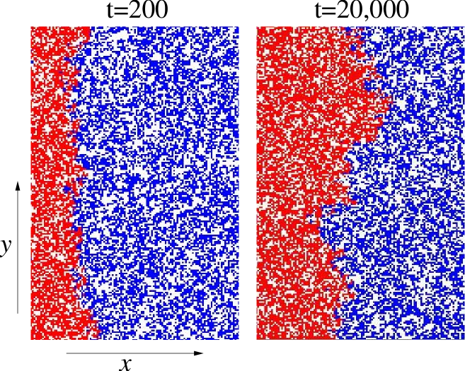
Figure 1: Snapshots of the moving and roughening front in the early-time regime ($t$$=$$200$ MCSS) and in the steady state ($t$$=$$20,000$ MCSS) for $\alpha_{1}$$=$$0.50$, $\alpha_{2}$$=$$0.70$, $\mu$$=$$0.20$, and $L_{y}$$=$$200$. White represents empty sites, while blue and red correspond to sites occupied by the residents and the invaders, respectively.

III Invasion as Propagation into an Unstable State

III.1 Mean-field equations and the asymptotic front velocity

Taking the master equation corresponding to transition rates in Eq. (1), and neglecting correlations between densities at different sites, yields dynamics of the ensemble-averaged local densities $\rho_{i}({\bf x},t)$$\equiv$$\langle n_{i}({\bf x},t)\rangle$. We obtain

$$\rho_{i}({\bf x},t+1)-\rho_{i}({\bf x},t) = \left[1-\rho_{1}({\bf x},t)-\rho_{2}({\bf x},t)\right]$$

$$\times\frac{\alpha_{i}}{4}\sum_{{\bf x^{\prime}}\epsilon{\rm nn}({\bf x})}\rho_{i}({\bf x^{\prime}},t) - \mu\rho_{i}({\bf x},t)\;.$$ (2)

where $i=1,2$. Taking the naive continuum limit of the above equations, one obtains the (coarse-grained) equations of motion

$$\partial_{t}\rho_{i}({\bf x},t) = \frac{\alpha_{i}}{4}\left[1-\rho_{1}({\bf x},t)-\rho_{2}({\bf x},t)\right]\nabla^{2}\rho_{i}({\bf x},t)$$ (3)

$$+ \alpha_{i}\left[1-\rho_{1}({\bf x},t)-\rho_{2}({\bf x},t)\right]\rho_{i}({\bf x},t)$$

$$- \mu\rho_{i}({\bf x},t)\;,$$

$i=1,2$. The spatially homogeneous solutions of these equations, $(\rho_{1}^{*},\rho_{2}^{*})$, are $(0,0),(1-\mu/\alpha_{1},0)$, and $(0,1-\mu/\alpha_{2})$. In the parameter regime of our interest, $\mu<\alpha_{1}<\alpha_{2}$, only the last solution $(0,1-\mu/\alpha_{2})$ is stable. Thus, the propagation of a front separating the stable $(0,1-\mu/\alpha_{2})$ (invader dominated) and unstable $(1-\mu/\alpha_{1},0)$ (resident dominated) regions amounts to propagation into an unstable state FISHER_37 ; KOLMOGOROV_37 ; Aronson_78 ; Dee_83 ; Saarloos_87 , a phenomenon that has generated a vast amount of literature Saarloos_03 since the original papers by Fisher FISHER_37 and Kolmogorov et al. KOLMOGOROV_37 . At the level of the mean-field equations, the front is “pulled” by the leading edge into the unstable state. Then, for a sufficiently sharp initial density profile MURRAY_03 ; Saarloos_03 , the asymptotic velocity is determined by the infinitesimally small density of invaders that intrude into the linearly unstable region dominated by the resident species. Linearizing Eqs. (3) about the unstable state, $\rho_{1}=1-\mu/\alpha_{1}+\phi_{1}$, $\rho_{2}=\phi_{2}$, one immediately obtains for the density of invaders

$$\partial_{t}\phi_{2}({\bf x},t)=\frac{\mu}{4}\frac{\alpha_{2}}{\alpha_{1}}\nabla^{2}\phi_{2}({\bf x},t)+\mu\left(\frac{\alpha_{2}}{\alpha_{1}}-1\right)\phi_{2}({\bf x},t)\;.$$ (4)

Performing standard analysis MURRAY_03 ; Dee_83 ; Saarloos_87 ; Saarloos_03 on the above equation, we obtain the asymptotic velocity of the “marginally stable” invading fronts

$$v^{*}=\frac{\mu}{\alpha_{1}}\sqrt{\alpha_{2}(\alpha_{2}-\alpha_{1})}.$$ (5)

The velocity $v^{*}$ above is the minimum velocity of a physically allowed travelling wave, permitted by Eqs. (4), and is actually realized by deterministic nonlinear reaction-diffusion dynamics for sufficiently sharp initial profiles MURRAY_03 ; Dee_83 ; Saarloos_87 ; Saarloos_03 . For further comparisons, we also note that the above asymptotic front velocity is approached as $v(t)=v^{*}-{\cal O}(1/t)$ Saarloos_03 . Also, as can be seen from Eq. (5), for small differences in the reproduction rates of the two species (a parameter of ecological significance), the front velocity scales as $v^{*}$$\sim$$(\alpha_{2}-\alpha_{1})^{\theta}$ with $\theta=1/2$.

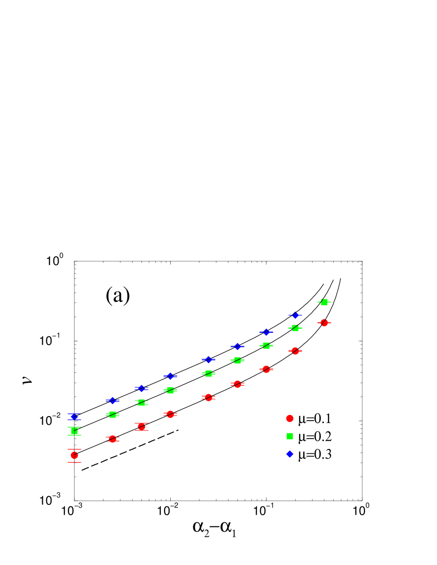
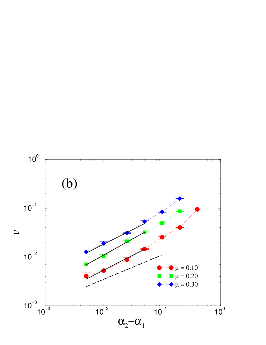
Figure 2: (Color online) (a) Asymptotic mean-field front velocities for three different mortality rates for fixed $\alpha_{2}$=$0.70$, as a function of the difference of propagation rates, $\alpha_{2}$$-$$\alpha_{1}$. Symbols are obtained by numerically iterating the nonlinear mean-field equations of motion [Eq. (2)]. The solid curves running through the data points are the analytically obtained velocities in the “leading edge” approximation [Eq. (5)], as described in the text. The straight dashed line indicates the slope $\theta$$=$$0.5$, corresponding to the exponent of an effective power law for small differences between the reproduction rates. (b) Asymptotic front velocities from Monte Carlo simulations for the individual-based stochastic model for fixed $\alpha_{2}$=$0.70$ as in (a), with $L_{y}=100$, for three values of $\mu$. The solid straight lines are the best-fit effective power laws in the region where the difference between the reproduction rates is small, corresponding to $\theta=0.61\pm 0.04$, $\theta=0.66\pm 0.04$, and $\theta=0.60\pm 0.04$ for $\mu$$=$$0.1$, $\mu$$=$$0.2$, and $\mu$$=$$0.3$, respectively. For comparison, the straight dashed line corresponds to the effective power law of the mean-field case with an exponent $\theta$=$0.5$.

It is important to note that the front velocity given by Eq. (5), obtained by linearizing Eq. (3), fully reproduces the velocity obtained by numerically iterating the non-linear continuous-density mean-field equations [Eq. (2)], as can be seen in Fig. 2(a). This is a generic and powerful feature of deterministic pulled fronts where, despite the non-linearity of the full dynamics, velocities are completely determined by the leading edge MURRAY_03 ; Saarloos_03 .

III.2 Monte Carlo results for the front velocity

We now present results for the discrete individual-based stochastic model defined by the transition rates Eq. (1). We found that the front velocity is much smaller than that of the mean-field approximation as shown in Fig. 2(b) [cf. Fig. 2(a)]. Further, for small differences in the reproduction rates, the velocity is described by an effective power law $v^{*}$$\sim$$(\alpha_{2}-\alpha_{1})^{\theta}$ with $\theta\stackrel{{\scriptstyle\sim}}{{>}}0.6$ [Fig. 2(b)], slightly, but distinctly, greater than the exponent $\theta$$=$$0.5$ of the mean-field case. Similar deviations from the mean-field exponent have been found in two-dimensional epidemic Warren_01 and reaction-diffusion models Moro_01 . The discreteness of the individuals Brunet_97 ; Kessler_98a ; Kessler_98b and noise Doering_03 ; Doering_05 have been shown to contribute to a velocity that is different from the mean-field description. The general belief is that fronts in stochastic individual-based (or particle) models are “pushed”, in the sense that the front velocity is determined by the full non-linear front region, instead of an infinitesimally small leading edge Saarloos_03 , a behavior predicted by the mean-field approximation. Our two-species model provides an example for this generic behavior.

An interesting feature of the invasion fronts is that their propagation velocity approaches the asymptotic value rather slowly (e.g. as ${\cal O}(1/t)$ in mean-field models Saarloos_03 ). Thus, from application point of view, it is important to establish how the front reaches its asymptotic velocity. In the next section, we are going to analyze both the temporal and finite-size approach toward the asymptotic front velocity, along with other universal characteristics (such interface roughening Barabasi_FCSG ; Zhang_review ) of the model, using the framework of scaling in non-equilibrium interfaces.

IV Interface Roughening and Corrections to the Asymptotic Front Velocity

IV.1 Dynamic scaling

To extract the scaling properties of the roughening of the front, as can be seen in Fig. 1, we analyze the width of the front

$$\langle w^{2}(L_{y},t)\rangle=\left\langle\frac{1}{L_{y}}\sum_{y=1}^{L_{y}}[h_{y}(t)-\overline{h}(t)]^{2}\right\rangle\;,$$ (6)

where $h_{y}(t)$ is defined as the location of the leading individual in row $y$ for the invading species. In what follows, we define $L\equiv L_{y}$, and investigate the scaling properties of the width $\langle w^{2}(L,t)\rangle$ within the standard framework of dynamic scaling of non-equilibrium interfaces Barabasi_FCSG ; Zhang_review .

The temporal and system-size scaling of the width $\langle w^{2}(L,t)\rangle$ typically identifies the universality class of the growing front. In finite systems, the width grows as $\langle w^{2}(L,t)\rangle$$\sim$$t^{2\beta}$ from early to intermediate times. At a system-size-dependent crossover time, $t_{\times}$$\sim$$L^{z}$, it saturates (reaches steady state) and scales as $\langle w^{2}_{sat}\rangle\equiv\langle w^{2}(L,\infty)\rangle\sim L^{2\alpha}$, where $L$ is the transverse linear system size. $\alpha$, $\beta$, and $z$ are referred to as the roughness, growth, and dynamic exponents, respectively. Further, these exponents are not independent, but obey the scaling relation $\alpha=\beta z$. The above temporal and system-size behavior, with the appropriate crossover time, can be captured by the Family-Vicsek scaling form FV

$$\langle w^{2}(L,t)\rangle=L^{2\alpha}f(t/L^{z}).$$ (7)

For small values of its argument, $f(x)$ behaves as a power law, while for large arguments it approaches a constant

$$f(x)=\left\{\begin{array}[]{ll}x^{2\beta}&\mbox{for $x\ll 1$}\\ {\rm const.}&\mbox{for $x\gg 1$}\end{array}\right.\;,$$ (8)

yielding the scaling behavior of the width in the growth and steady-state regime, provided the scaling relation for the exponents, $\alpha=\beta z$, holds.

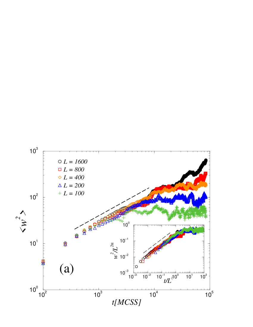
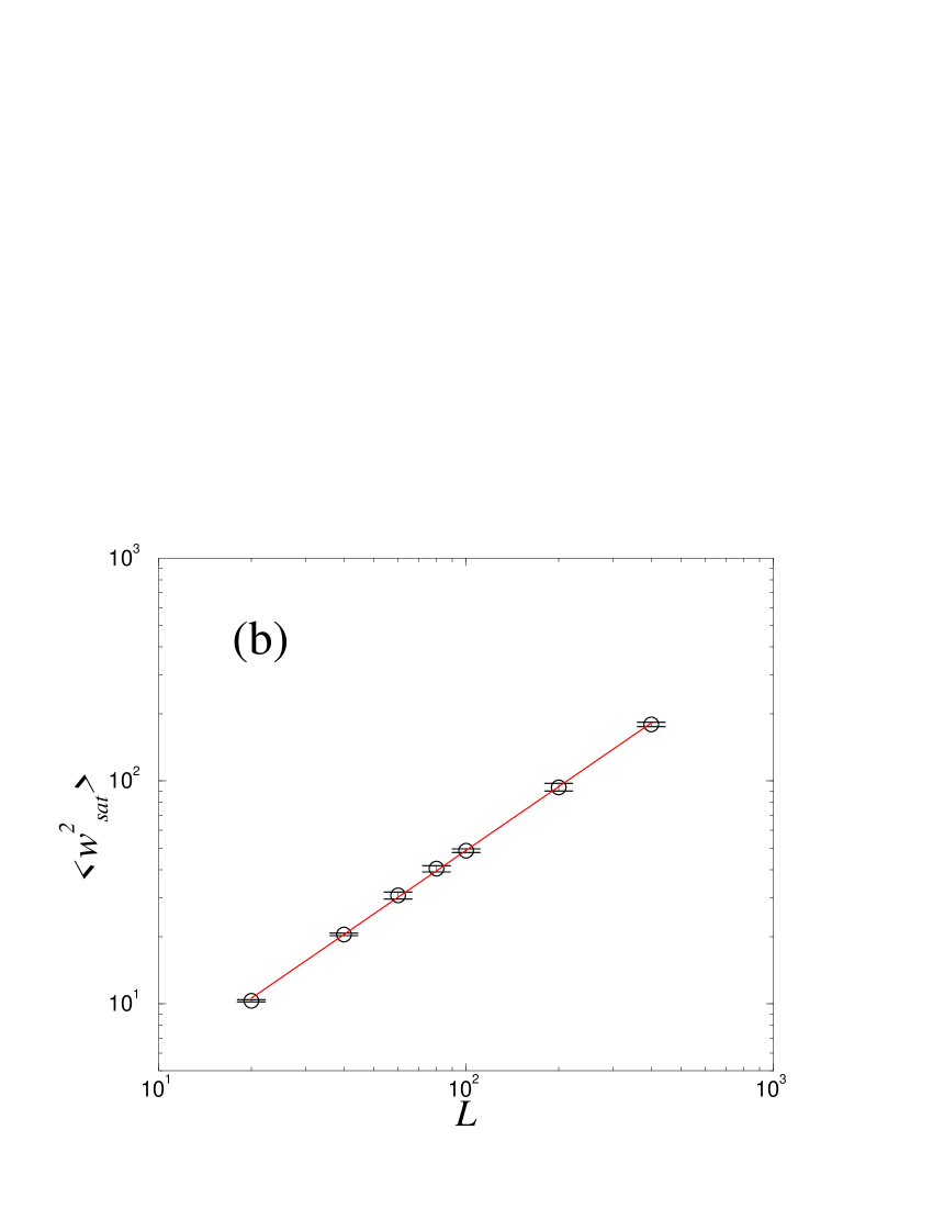
Figure 3: (Color online) (a) The average width as a function of time (on log-log scales) for various system sizes, averaged over $20$ independent realizations, for $\alpha_{1}=0.70$, $\alpha_{2}=0.80$, and $\mu=0.10$. The dashed line corresponds to the one-dimensional KPZ power law with the exponent $2\beta=2/3$. The inset shows the scaled plot, $\langle w^{2}(L,t)\rangle/L^{2\alpha}$ vs. $t/L^{z}$ using the one-dimensional KPZ exponents. (b) Steady-state width as a function of the system size, $L(\equiv L_{y})$, for the same clonal propagation and mortality rates as in (a). The solid line corresponds to the best-fit power law with the exponent $2\alpha=0.95\pm 0.01$.

As as shown in Figs. 3, our results show reasonable agreement with the exponents of the well-known KPZ universality class ($\beta$$=$$1/3$, and $\alpha$$=$$1/2$) Barabasi_FCSG ; Zhang_review ; KPZ_86 . Further, the scaled width, $\langle w^{2}(L,t)\rangle/L^{2\alpha}$ vs. $t/L^{z}$ produces good data collapse, as suggested by Eq. (7), and confirms dynamic scaling for the invasion process [Fig. 3(a) inset].

IV.2 Steady-state width distribution

For further analysis, we also constructed the full distributions $P(w^{2})$ of the steady-state width for different system sizes [i.e., the normalized histograms of the width obtained from the steady-state time series]. This observable typically provides an additional strong signature of the underlying universality class of the fluctuating and growing interface foltin . In particular, for the one-dimensional KPZ class, it has been obtained analytically foltin and can be written in the generic scaling form $P(w^{2})=\langle w^{2}\rangle^{-1}\Phi(w^{2}/\langle w^{2}\rangle)$ with

$$\Phi(x)=\frac{\pi^{2}}{3}\displaystyle\sum_{n=1}^{\infty}(-1)^{n-1}n^{2}e^{-(\pi^{2}/6)n^{2}x}.$$ (9)

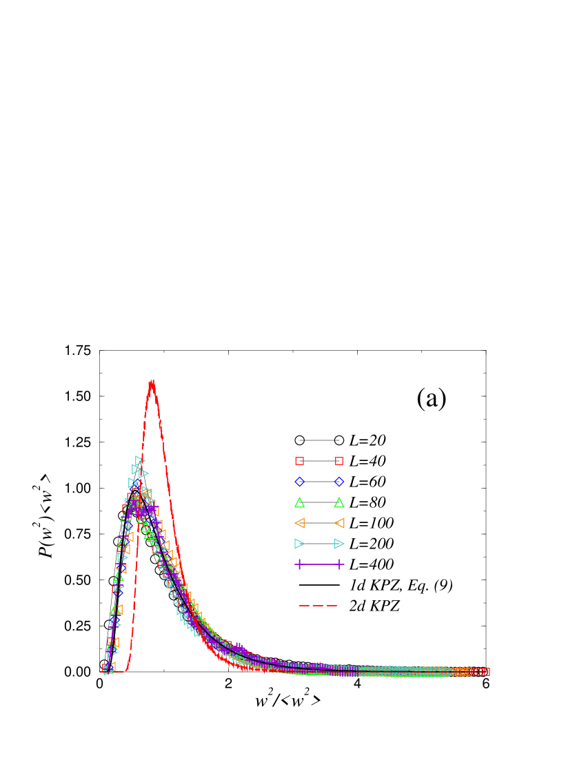
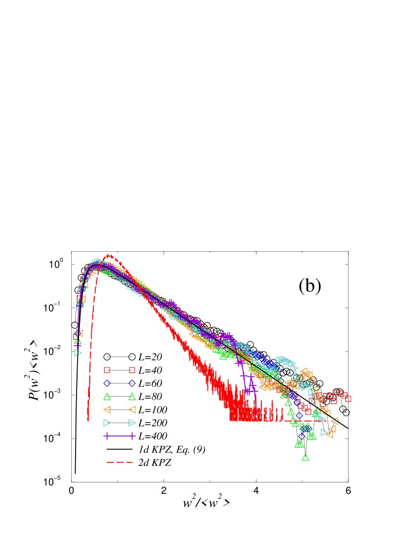
Figure 4: (Color online) (a) Steady-state width distributions for $\alpha_{1}$$=$$0.70$, $\alpha_{2}$$=$$0.80$, and $\mu$$=$$0.10$ for various system sizes $L$. The solid curve is the scaled analytic width distribution of the one-dimensional KPZ class foltin , Eq. (9). For comparison, the two-dimensional scaled KPZ width distribution is also shown, as obtained in Ref. Marinari_PRE90 (b) The same as (a) but on log-normal scales.

In Fig. 4 we show the scaled width distribution $P(w^{2})\langle w^{2}\rangle$ vs. $w^{2}/\langle w^{2}\rangle$ for various system sizes and compare it with the above analytic scaling function $\Phi(x)$. Our data, again, strongly suggest that propagating planar fronts in our two-species invasion model belong to the one-dimensional KPZ universality class. The large deviations and data scattered around peaks of the distributions are due to sampling error. Steady-state time series for larger systems become strongly correlated, and so require excessively long simulations to generate sufficiently large statistically independent samples. Fig. 4 also shows the KPZ width distribution in two transverse dimensions Marinari_PRE90 , offering a comparison suggested by a recent, somewhat counterintuitive conjecture Saarloos_PRL01 . That conjecture suggests that fronts which are pulled in the mean-field limit, belong to the one higher dimensional KPZ class than one would normally expect (i.e., two instead of one transverse dimension in our model). We give more discussion on this topic aspect in Sec. V.

IV.3 Temporal and finite-size corrections to the asymptotic front velocity

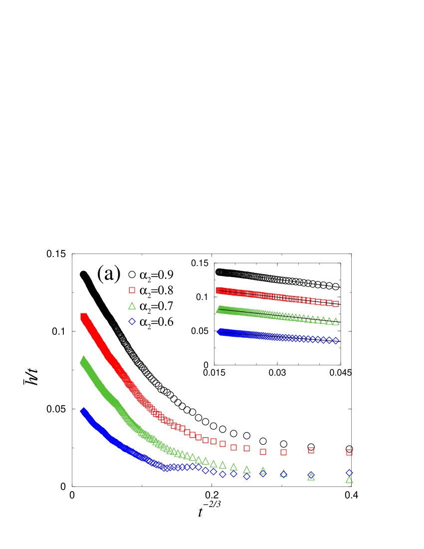
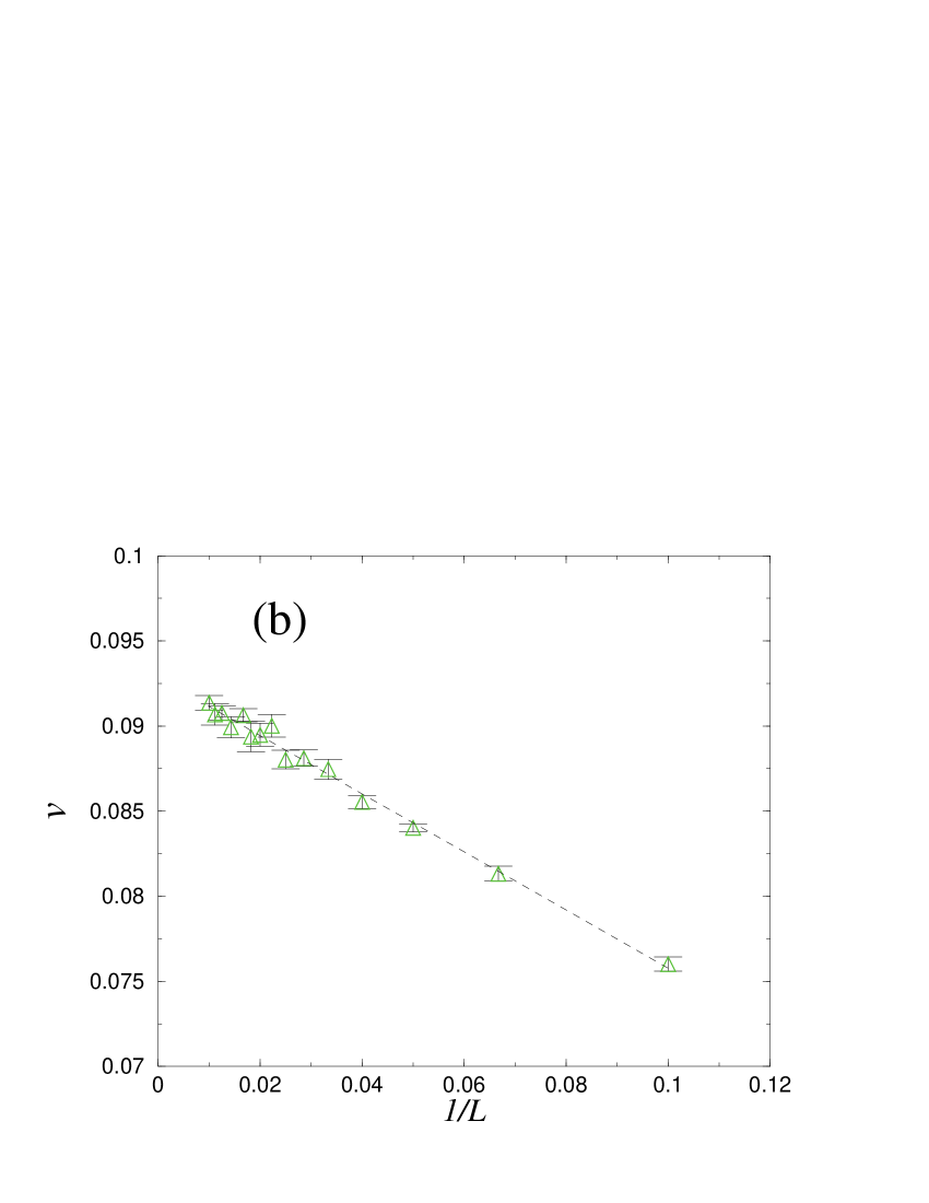
Figure 5: (Color online) (a) Temporal corrections to the asymptotic front velocity for $L$$=$$800$ for different values of $\alpha_{2}$, with $\alpha_{1}$$=$$0.50$ and $\mu$$=$$0.20$. The horizontal (time) axis is scaled as $t^{-2/3}$, motivated by the form of the corrections of the one-dimensional KPZ class [Eq. (11)]. The inset enlarges the regime of (a) where the universal temporal corrections follow the KPZ behavior. The straight solid lines correspond to the linear scaling as a function of $t^{-2/3}$. (b) Finite-size corrections to the asymptotic velocity as a function of $L^{-1}$, motivated by the universal corrections of the one-dimensional KPZ class, for $\alpha_{1}$$=$$0.50$, $\alpha_{2}$$=$$0.70$, and $\mu$$=$$0.20$. The straight dashed line corresponds to the linear behavior as a function of $1/L$.

Although the actual value of the velocity of the invading front is not universal, Krug and Meakin Krug_90 showed that the forms of the temporal and finite-size corrections of the front velocity, $v(L,t)=d\overline{h}(L,t)/dt$, are universal. More specifically, corrections to the asymptotic front velocity $v^{*}$ are given by Krug_90

$$v(L,t)=\left\{\begin{array}[]{lll}v^{*}-c_{1}t^{-2(1-\alpha)/z}&\mbox{for}&t\ll L^{z}\\ v^{*}-c_{2}L^{-2(1-\alpha)}&\mbox{for}&t\gg L^{z}\end{array}\right.\;,$$ (10)

where $\alpha$ and $z$ are the roughness and dynamic exponents characterizing the universality class of the model, and $c_{1}$ and $c_{2}$ are non-universal constants depending on the parameters and microscopic details of the specific model. Translating their results to the easily measurable quantity $\overline{h}(t)/t$ (by integrating the above equation with respect to time and dividing the result by $t$), one also has

$$\frac{\overline{h}(L,t)}{t}=\left\{\begin{array}[]{lll}v^{*}-c_{1}^{\prime}t^{-2(1-\alpha)/z}&\mbox{for}&t\ll L^{z}\\ v^{*}-c_{2}L^{-2(1-\alpha)}&\mbox{for}&t\gg L^{z}\end{array}\right.\;,$$ (11)

where $c_{1}^{\prime}=c_{1}z/(z+2\alpha-2)$. In particular, for the one-dimensional KPZ class, $2(1-\alpha)/z=2/3$ and $2(1-\alpha)=1$. Thus, the early-time temporal, and late-time finite-size corrections scale as ${\cal O}(t^{-2/3})$ and ${\cal O}(L^{-1})$, respectively. Our data for the velocity of the propagating front in the two species-invasion model follows these corrections very closely [Fig. 5], offering additional evidence that the front belongs to the one-dimensional KPZ class. Also, note that the temporal relaxation of the front velocity is in contrast to mean-field results where pulled fronts exhibit ${\cal O}(t^{-1})$ corrections to the asymptotic velocity Saarloos_03 .

V Discussion and Summary

We studied front propagation in a two-species model for ecological invasion with preemptive competition, applicable to clonal plants. We performed dynamic Monte Carlo simulations using the local transition rules [Eq. (1)] for initially flat linear fronts. We found the front velocity significantly smaller than that of the mean-field approximation. Also, for small differences between local reproduction rates, the asymptotic front velocity scales as an effective power law $v^{*}$$\sim$$(\alpha_{2}-\alpha_{1})^{\theta}$ with $\theta\stackrel{{\scriptstyle\sim}}{{>}}0.6$, an exponent slightly, but noticeably different from the mean-field value $\theta=0.5$. The discreteness of the individuals Brunet_97 ; Kessler_98a ; Kessler_98b in our lattice model (or, the effective density cutoffs in a continuum description) and noise Doering_03 ; Doering_05 have been shown to contribute to the deviations from the mean-field results. More specifically, fronts in stochastic individual-based models, which in the mean-field limit converge to a pulled front solution, are instead “pushed”. Therefore, the front velocity is determined by the entire non-linear front region, instead of the infinitesimally small leading edge alone Saarloos_03 . Our model is an example for this type of behavior.

We also investigated the universal features of the roughening of the propagating front, separating the invaders and the residents. We found that the front roughening in our two-species invasion model belongs to the one-dimensional KPZ class. We must also place our results in the context of a recent conjecture by Tripathy et al. Saarloos_PRL01 that propagating fronts, which in the mean-field limit are “pulled”, exhibit KPZ scaling on a $(d_{\perp}$$+$$1)$ dimensional “substrate” (where $d_{\perp}$ is the dimension of the space transverse to the direction of propagation), as opposed to the naive expectation of a $d_{\perp}$-dimensional KPZ growth (i.e., two-dimensional instead of one-dimensional in our case.) That conjecture Saarloos_PRL01 was based on field-theoretical arguments, but were subsequently shown by Moro Moro_01 to apply only to systems where stochastic effects are due to external fluctuations (such as, fluctuations in the parameters of the model). Most recently, it was argued Moro_01 ; Saarloos_03 and demonstrated Moro_01 that, in fact, fronts which in the mean-field limit are “pulled”, in the presence of internal fluctuations (i.e., systems with stochastic particle dynamics), belong to the “usual” $d_{\perp}$-dimensional KPZ universality class. While corrections-to-scaling effects and system size-limitations can often hinder a high-precision determination of the exponents associated with interface roughening, the width distributions provide a very strong signature and aid in determining the universality class of the interface foltin . To that end, we included the two-dimensional width distribution Marinari_PRE90 in Figs. 4, supporting the conclusion that our two-species invasion model with stochastic particle dynamics exhibits “standard” (one-dimensional) KPZ roughening, in agreement with the most recent generic arguments Moro_01 ; Saarloos_03 .

As noted in the Introduction, although linear fronts are somewhat artificial in the context of ecological invasion, they do offer insight into more realistic scenarios. Consider, for example, that an advantageous allele or a competitively superior species is introduced through mutation within YKC_05 ; OBYKAC_05 or through geographic dispersal to KC_JTB ; OAKC_SPIE a resident population, respectively. Introductions occur rarely and stochastically in both space and time. Thus, small clusters of an advantageous allele or superior species can randomly “nucleate” and subsequently grow. We have shown YKC_05 ; OBYKAC_05 ; KC_JTB ; OAKC_SPIE that the time evolution of such systems can be well described within the framework of homogeneous nucleation and growth. The growing clusters, on average, have radial symmetry and reach an asymptotic velocity $v^{*}$ for sufficiently long times. The corrections to the asymptotic radial velocity of these circular fronts have two contributions: First, the typical length of the perimeter of the cluster scales as $L(t)\sim 2\pi R(t)\sim t$, where $R(t)$ is the radius of the cluster. Since $z>1$, $t\ll L^{z}(t)$ for late times, i.e., the relevant KPZ correction for radially growing clusters is always of ${\cal O}(t^{-2/3})$ Krug_90 . Second, for long times, when the radius of the cluster is sufficiently large, the curvature introduces an additional ${\cal O}(R^{-1})\sim{\cal O}(t^{-1})$ correction, subdominant to the above KPZ correction. Thus, circular fronts are expected to reach the same asymptotic velocity as their linear counterpart, with the same leading-order ${\cal O}(t^{-2/3})$ corrections for late times.

- (1) J.D. Murray: Mathematical Biology I and II, 3rd edition (Springer-Verlag, New York, 2002, 2003).
- (2) J. Riordan, C.R. Doering, and Daniel ben-Avraham, Phys. Rev. Lett. 75, 565 (1995).
- (3) E. Ben-Naim, Europhys. Lett. 69, 671 (2005).
- (4) R.A. Fisher, Annals of Eugenics 7, 355 (1937).
- (5) A.N. Kolmogorov, I. Petrovsky, and N. Piskounov, Moscow Univ. Bull. Math. 1, 1 (1937).
- (6) Metz et al. in The Geometry of Ecological Interactions, edited by U. Dieckmann, R. Law, and J.A.J. Metz (Cambridge University Press, Cambridge, UK, 2000).
- (7) R. Durrett and S.A. Levin, S.A., Phil. Trans. R. Soc., London B 343, 329 (1994).
- (8) G. Korniss and T. Caraco, J. Theor. Biol. 233, 137 (2005).
- (9) L. O’Malley, J. Basham, J.A. Yasi, G. Korniss, A. Allstadt, and T. Caraco, Theor. Popul. Biol. (2005, in press); arXiv.org: q-bio/0602023.
- (10) J.B. Shurin, P. Amarasekare, J.M. Chase, R.D. Holt, M.F. Hoopes, and M.A. Leibold, J. Theor. Biol. 227, 359 (2004).
- (11) P. Amarasekare, Ecol. Lett. 6, 1109 (2003).
- (12) D.W. Yu and H.B. Wilson, Am. Nat. 158, 49 (2001).
- (13) D.E. Taneyhill, Ecol. Monogr. 70, 495 (2000).
- (14) B. Oborny, G. Meszéna and G. Szabó, Oikos 109, 291 (2005).
- (15) A.-L. Barabási and H.E. Stanley, Fractal Concepts in Surface Growth (Cambridge University Press, Cambridge, 1995).
- (16) T. Halpin-Healy and Y.-C. Zhang, Phys. Rep. 254, 215 (1995).
- (17) A.K Sakai and T.A Burris, Ecology 66, 1921 (1985).
- (18) J.A. Kemperman, and B.V. Barnes, Can. J. Botany 54, 2603 (1976).
- (19) J.A. Yasi, G. Korniss, and T. Caraco, in Computer Simulation Studies in Condensed Matter Physics XVIII, edited by D.P. Landau, S.P. Lewis, and H.-B. Schüttler, Springer Proceedings in Physics (Springer-Verlag, Berlin, in press); arXiv:cond-mat/0505523 (2005).
- (20) L. O’Malley, A. Allstadt, G. Korniss, T. Caraco: in Fluctuations and Noise in Biological, Biophysical, and Biomedical Systems III, edited by N.G. Stocks, D. Abbott, and R.P. Morse, Proceedings of SPIE Vol. 5841 (SPIE, Bellingham, WA, 2005) pp. 117–124.
- (21) A. N. Kolmogorov, Bull. Acad. Sci. USSR, Phys. Ser. 1, 355 (1937); W. A. Johnson and R. F. Mehl, Trans. Am. Inst. Mining and Metallurgical Engineers 135, 416 (1939); M. Avrami, J. Chem. Phys. 7, 1103 (1939); J. Chem. Phys. 8, 212 (1940); J. Chem. Phys. 9, 177 (1941).
- (22) L. O’Malley, B. Kozma, G. Korniss, Z. Rácz, and T. Caraco, in Computer Simulation Studies in Condensed Matter Physics XIX, edited by D.P. Landau, S.P. Lewis, and H.-B. Schüttler, Springer Proceedings in Physics (Springer-Verlag, Berlin, in press); arXiv:q-bio.PE/0603013 (2006).
- (23) M. Kardar, G. Parisi and Y. Zhang, Phys. Rev. Lett. 56, 889 (1986).
- (24) T.E. Harris, Ann. Prob. 2 969 (1974).
- (25) H. Hinrichsen, Adv. Phys. 49, 815 (2000).
- (26) D.G. Aronson and H. F. Weinberger, Adv. Math. 30, 33 (1978).
- (27) G. Dee and J. S. Langer, Phys. Rev. Lett. 50, 383 (1983).
- (28) W. van Saarloos, Phys. Rev. Lett. 58, 2571 (1987).
- (29) W. van Saarloos, Phys. Rep. 386, 29 (2003).
- (30) C.P. Warren, G. Mikus, E. Somfai, and L.M. Sander, Phys. Rev. E 63, 056103 (2001).
- (31) E. Moro, Phys. Rev. Lett. 87, 238303 (2001).
- (32) E. Brunet and B. Derrida, Phys. Rev. E 56, 2597 (1997)
- (33) D.A. Kessler, Z. Ner, and L.M. Sander, Phys. Rev. E 58, 107 (1998).
- (34) D.A. Kessler and H. Levine, Nature 394, 556 (1998).
- (35) C.R. Doering and C. Mueller, P. Smereka, Physica A 325, 243 (2003).
- (36) J.G. Conlon and C.R. Doering, J. Stat. Phys. 120, 421 (2005).
- (37) F. Family and T. Vicsek, J. Phys. A 18, L75 (1985).
- (38) G. Foltin, K. Oerding, Z. Rácz, R.L. Workman, and R.K.P. Zia, Phys. Rev. E 50, R639 (1994).
- (39) G. Tripathy, A. Rocco, J. Casdemunt, and W. van Saarloos, Phys. Rev. Lett. 86, 5215 (2001).
- (40) E. Marinari, A. Pagnani, G. Parisi, and Z. Rácz, Phys. Rev. E 65, 026136 (2002).
- (41) J. Krug and P. Meakin, J. Phys. A: Math. Gen. 23, L987 (1990).