Asymptotic analysis and analytical solutions of a model of cardiac excitation

Abstract

We describe an asymptotic approach to gated ionic models of single-cell cardiac excitability. It has a form essentially different from the Tikhonov fast-slow form assumed in standard asymptotic reductions of excitable systems. This is of interest since the standard approaches have been previously found inadequate to describe phenomena such as the dissipation of cardiac wave fronts and the shape of action potential at repolarization. The proposed asymptotic description overcomes these deficiencies by allowing, among other non-Tikhonov features, that a dynamical variable may change its character from fast to slow within a single solution. The general asymptotic approach is best demonstrated on an example which should be both simple and generic. The classical model of Purkinje fibers (Noble, 1962) has the simplest functional form of all cardiac models but according to the current understanding it assigns a physiologically incorrect role to the Na current. This leads us to suggest an “Archetypal Model” with the simplicity of the Noble model but with a structure more typical to contemporary cardiac models. We demonstrate that the Archetypal Model admits a complete asymptotic solution in quadratures. To validate our asymptotic approach, we proceed to consider an exactly solvable “caricature” of the Archetypal Model and demonstrate that the asymptotic of its exact solution coincides with the solutions obtained by substituting the “caricature” right-hand sides into the asymptotic solution of the generic Archetypal Model. This is necessary, because, unlike in standard asymptotic descriptions, no general results exist which can guarantee the proximity of the non-Tikhonov asymptotic solutions to the solutions of the corresponding detailed ionic model.

¹ Department of Mathematical Sciences, University of Liverpool, Liverpool L69 7ZL, UK

² Deceased 25/03/2007. Last affiliation: Institute of Mathematical Problems of Biology of the Russian Academy of Sciences, Pushchino, and the Pushchino branch of the Moscow State University, Russia

³ Current address: Department of Mathematics, University of Glasgow, Glasgow G12 8QW, UK

Keywords excitability, action potential, asymptotic methods, singular perturbations.

1 Introduction

1.1 Physiological and mathematical motivation

Mechanical activity of the heart is controlled by electrical excitation of cardiac cells, characterized by “action potentials” (APs) across their membranes. Abnormalities of cardiac rhythm are a major public health hazard [47], and great efforts are directed to the mathematical modelling of APs. Investigations at various levels of membrane, cellular and myocardial organisation have lead to the development of a large number of detailed ionic cardiac models (for reviews, see e.g. [20, 23, 26, 45, 14]) for various types of cardiac cells. These detailed models are realistic in the sense that they demonstrate good agreement with experimental data available to their authors at the time of creating the model. There even exists an optimistic view that with the help of detailed cardiac computational models “it will soon be possible to do in silico experiments that would be impossible, difficult or unethical in animals or patients” [14].

In reality however, detailed ionic models of cardiac excitation are immensely complicated. Their analytical solution is impossible while their simulations are expensive especially in three dimensions. Thus, numerous attempts have been made to construct simplified mathematical models of cardiac action potentials (APs); for examples, see [43, 25, 3, 18, 34, 16, 21, 17, 6]. Detailed ionic cardiac models were initially constructed as variations of the spectacularly successful Hodgkin-Huxley model of nerve excitability [22]. In a similar way the most simplified cardiac models are often based on the elegant FitzHugh-Nagumo two-variable reduction [19, 31] of the Hodgkin-Huxley model. A typical way to create a simplified model is either to make an appropriate functional generalization of the FitzHugh-Nagumo system, or truncate a detailed ionic models. Then the modellers proceed to fit the parameters of their simplified models to reproduce the AP shape or other selected properties of the chosen detailed ionic model.

This modelling approach has an obvious flaw, as such simplified models are not reliable outside the range of phenomena which they have been fitted to reproduce. So it would be desirable to derive a simplified model from a detailed model, based on a well defined set of verifiable assumptions. One possible way to do that is via asymptotic methods, which would utilize small parameters available in the detailed model.

More importantly, reducing the number of equations in the model often delivers only minor reduction of its computational complexity. Paradoxically, the better a simplified model is, the better it reproduces another difficult feature of realistic models, their stiffness. That is, detailed ionic models typically have small parameters which considerably complicate their simulation. However it would be natural to try and eliminate those parameters by asymptotic methods, and resulting problems without small parameters should be much easier for computational study.

Yet another paradoxical property of ionic models is that increasing the number of physiological details does not necessarily make the models more reliable, as experimental data are not always sufficient for unequivocal identification of model parameters. As argued by Cherry and Fenton [13], detailed ionic models of the same types of cells in the same species, but developed by different authors, may disagree significantly. Thus there is a demand in modelling practice for models that would be realistic physiologically but independent on experimentally unreliable details, i.e. depend on fewer parameters. Again, one possible way to create such a model is to simplify a “too detailed” model by eliminating exceeding details by some sort of asymptotic procedure.

So there is more than one serious reason to look more carefully into the small parameters in detailed ionic models. The progress in this direction was hampered for some time by implicit assumption, induced by the success of the FitzHugh-Nagumo system, that the essential properties of cardiac APs can be captured by dynamical systems of the type

$${\epsilon}\frac{\mathrm{d}{x}}{\mathrm{d}{t}}={f}({x},{y}),\quad\frac{\mathrm{d}{y}}{\mathrm{d}{t}}={g}({x},{y}),\qquad{x}\in\mathbb{R}^{k},\;{y}\in\mathbb{R}^{l},\;{\epsilon}\ll 1,$$ (1)

in which some of the dynamic variables are fast (${x}$) while others are slow (${y}$) and where ${\epsilon}>0$ is a small parameter. The asymptotic structure of (1) is mathematically very convenient. Indeed, the presence of the small parameter ${\epsilon}$ at the derivatives allows to “dissect” equations (1), in the leading order in ${\epsilon}$, into a slow-time (degenerate) subsystem

$$0={f}({x},{y}),\quad\frac{\mathrm{d}{y}}{\mathrm{d}{t}}={g}({x},{y}),$$ (2)

and a fast-time subsystem

$$\frac{\mathrm{d}{x}}{\mathrm{d}{T}}={f}({x},{y}),\quad\frac{\mathrm{d}{y}}{\mathrm{d}{T}}=0,$$ (3)

with ${T}={\epsilon}\,{t}$, which are much easier to study. It is assumed that the fast subsystem (3) has, for all relevant values of $v$, no attractors but isolated, asymptotically stable equilibria. There exist a classical theory stating the general conditions which guarantee that, in the limit of ${\epsilon}\to 0$, any finite segment of the graph of solution of the full equations (1) approaches uniformly to that of the degenerate subsystem (2) which, in turn, consists of slow-motion parts and fast-motion parts separated by junction points. The slow-motion parts are on the $l$-dimensional “slow manifold” determined by the first $k$ equations in (2) and the fast-motion parts are arcs of trajectories of (3) within leaves of the “fast foliation” ${y}=\mathrm{const}$ [30, p.173]. A central result of the theory of slow-fast systems is the Tikhonov theorem [41].

A paradigm for applying the theory of fast-slow systems to biological excitability has been laid down by Zeeman [46]. His fundamental idea is a generalization of the FitzHugh-Nagumo view and states that the resting state is the unique and globally stable equilibrium of the full system, but in the fast subsystem, it is only one of three equilibria. There is another stable equilibria corresponding to the excited state, and the two stable equilibria are separated by an unstable equilibrium which thereby represents the threshold of excitation. The repolarization from the excited state, which is an equilibrium in the fast subsystem but not in the full system, to the resting state which is the true equilibrium, happens via the slow system, and its details, i.e. the shape of the action potential, depends on the structure of the slow manifold.

Thus, we refer to excitable systems with the asymptotic structure of equations (1) as FitzHugh-Nagumo type or Tikhonov-Zeeman systems.

Extension of this ideology to spatially-extended excitable systems produces a very attractive and promising asymptotic theory, see e.g. [42] for a review. In this theory, description of excitation waves is decoupled into description of fast motion of their sharp “fronts” and “backs”, and description of slow parts of APs outside fronts and backs. After appropriate rescaling, both the fast and the slow subsystems do not have the small parameter in them, so their numerical simulation could be implemented efficiently.

However, this attractive theory was never really applied to cardiac ionic models. It appears that FitzHugh-Nagumo type systems fail, in principle, to reproduce some qualitative features of ionic models. Here are some examples.

Features of cardiac excitability:

1. Slow repolarization. Cardiac APs tend to have very fast upstrokes and much slower other phases, including repolarization (“downstroke”). In the asymptotic limit ${\epsilon}\to 0$, a FitzHugh-Nagumo system of the form (1) with $l=1$ will have a fast, i.e. duration ${t}\sim{\epsilon}$, upstroke of the action potential will have also fast, $\sim{\epsilon}$ downstroke. In principle, this can be avoided if the slow manifold, defined by ${f}({x},{y})=0$, has a cusp singularity with respect to foliation ${y}=\mathrm{const}$, which is theoretically possible if $l\geq 2$ [46]. However, our attempts to identify such a cusp singularity in cardiac equations have not been successful [39, 12]

2. Slow subthreshold response. An excitable system reacts to a subthreshold stimulus by an immediate return to the resting state. In the asymptotic limit ${\epsilon}\to 0$, a FitzHugh-Nagumo system of the form (1) will have both subthreshold return and super-threshold upstroke very fast, ${t}\sim{\epsilon}$. However, subthreshold return in real cells and realistic models has speed comparable to the slow stages of the AP, i.e. much slower than the upstroke.

3. Fast accommodation. If the stimulus is applied not instantly but gradually, then the threshold of excitation may increase, and if the perturbation is too slow, the system may fail to generate AP altogether (phenomenon known as accommodation). FitzHugh-Nagumo systems demonstrate accommodation but only if the time scale of the stimulus is comparable to the duration of the AP. In real cells and realistic models, accommodation is observed for much faster stimuli, comparable more to the upstroke duration than to the AP duration.

4. Variable peak voltage. The maximum of the AP in a single cell does not, in the first approximation, depend on the way the AP has been elicited. Moreover, the asymptotic theory of [42] predicts that the maximum of the AP in a propagating wave will be the same as in a single cell. However, in real cells and in realistic models the maximum of AP does depend on the mode of excitation, and in the propagating AP it could be significantly different than in a single cell.

5. Front dissipation. The fast accommodation of realistic models has an interesting consequence for propagating waves. If excitability ahead of the wave is temporarily blocked by a transient process, the wave will expire if the block lasts too long. In a FitzHugh-Nagumo type system, this will happen if the duration of the block equals the duration of the wave; that is, the wave will cease when its “length”, understood as the spatial size of the excited zone, has decreased to zero [44]. In contrast, in ionic models the front looses its sharpness, “dissipates”, much sooner than AP finishes, and after that fails to propagate even though AP continues in many cells and the excitability of the tissue ahead of the wave has fully recovered [9, 11, 8].

In this article, we describe a non-Tikhonov asymptotic approach to cardiac excitation. Its purpose is to overcome the limitations of simplified models of FitzHugh-Nagumo type discussed above. The approach has already been used in some form in [38] to achieve numerically accurate prediction of the front propagation velocity (within 16 %) and its profile (within $0.7$ mV) for a realistic model of human atrial tissue [15]. The asymptotic reduction was sufficiently simple to allow the derivation of an analytical condition for propagation block in a re-entrant wave which was in an excellent agreement with results of direct numerical simulations of the realistic atrial ionic model. This has been achieved by considering only the “fast subsystem” of the full model.

Here we take a further step and present a complete asymptotic description of a simple cardiac excitation model, including both fast subsystem and slow subsystem, i.e. describing the whole AP rather than the upstroke only. A brief sketch of this description has been outlined in [10]. That sketch has left several questions unanswered, and the purpose of the present article is to fill in the gaps. The asymptotic reductions we propose are based on a well-defined and verifiable set of assumptions and in this sense they are “derived” from a detailed ionic model. We do not include arbitrary fitting parameters which limit the model to the reproduction of few hand-picked AP properties. All arbitrariness is restricted to choice of small parameters in the model, which is the key stage in any asymptotic approach. In our approach, the main small parameter occurs in an essentially different way from (1). Consequently, the results of the classical theory of slow-fast systems [30] are not applicable. In other words, there is no existing rigorous theory which can guarantee that the asymptotic solutions are close to the true solutions of the corresponding detailed ionic model. To deal with this issue, we formulate a caricature model which exactly duplicates the asymptotic structure of a detailed ionic model but allows exact analytical solution. We proceed to apply the asymptotic procedure to this caricature and to compare the exact and the asymptotic solutions in order to validate our approach.

To demonstrate our approach, we need to chose an appropriate gated ionic model. Such a selected model must satisfy two criteria. Firstly it should be as simple as possible. Secondly, it should have the generic structure similar to all or most of contemporary ionic models. The first requirement is best satisfied by the classical Noble model of excitability of cardiac Purkinje fibers [32]. This model has spawned generations of models of increasing accuracy and complexity up to modern models with more than sixty differential equations per single cell [24]. The Noble model, however, does not satisfy the second requirement. Indeed, while that model reproduces the AP of Purkinje fibers in detail, it does not correctly reflect their physiology. As the model was constructed before sufficient experimental data on the ionic currents became available [33], the inward sodium current was given the dual role of generating the upstroke and maintaining the plateau. To avoid this peculiarity and to ensure that our asymptotic procedure is sufficiently general, we propose an “Archetypal Model” (AM) which has the generic structure of modern cardiac models but keeps the functional simplicity of the the Noble model and is identical to it in the asymptotic limit. The asymptotic procedure is then demonstrated on the example of this Archetypal Model.

The structure of the paper is as follows. We conclude the Introduction with a short discussion of the procedure of parametric embedding which is an important instrument in our work. In section 2, we use a set of numerical observations to postulate a system of axioms for a non-Tikhonov parametric embedding of the Noble model. In section 3, we describe the AM and discuss its similarities with contemporary ionic models and then study the asymptotic limits of the AM and obtain analytical solutions in quadratures in these limits. In section 4, we formulate the exactly solvable “caricature” simplification of the AM. In section 5, we validate our general asymptotic results by a comparison of the limits of the exact solution of the caricature model to its solution in the asymptotic limit. We conclude by outlining the most essential features of our approach and discussing possibilities for its application.

In all asymptotics, we restrict consideration to the leading order, with the exception of Appendix A which is about a first-order correction.

Some parts of this work (subsections 1.2, 2.1, 2.3, 3.1, 3.2) appeared in a very brief form in [10] and are reproduced here in the full form, with additional details, for completeness and convenience of reference in the rest of the article; other parts (subsections 2.2, 2.4, sections 4 and 5 and appendices A, B and C ) are entirely new.

1.2 The procedure of parametric embedding

The nonlinear problems of physical, chemical and biological applications do not normally have parameters which are literally approaching zero within their normal range relevant to the application. Hence, a typical practical approach to asymptotic reduction is to identify a “small constant”, say $a$, in the model and to replace it by a parameter $\epsilon$, so that the original problem corresponds to $\epsilon=a$, whereas the asymptotic formulae are obtained in the limit $\epsilon\rightarrow 0$. A mathematically equivalent modification of this procedure is based on the following

Definition  A parametric embedding with parameter $\epsilon$ of a function $f(x)$ is any function $\underline{{f}}(x;\epsilon)$ such that $\underline{{f}}(x,1)=f(x)$ for all $x\in\mathrm{dom}(f)$. A parametric embedding in the context of $\epsilon\rightarrow 0$ is called asymptotic embedding. An embedding of a dynamical system corresponds to an embedding of its generating vector field or map.

Thus, the “small constant” $a$ is replaced by $\epsilon a$, and then the original problem corresponds to $\epsilon=1$ while the asymptotic analysis is performed in the limit $\epsilon\rightarrow 0$. As long as $a$ is a nonzero constant, the limits $\epsilon\to$ and $\epsilon a\to$ are mathematically equivalent. The purpose of the above definition is uniformity, especially when the small parameters appear in more than one place in the equations. From this perspective, the algorithm of obtaining an approximation using, say, a partial sum of an asymptotic series is: the power series in $\epsilon$ is truncated to a selected number of terms, and then $\epsilon=1$ substituted in the result. When applied formally, this may look counter-intuitive, and yet for reasons explained above, this is precisely equivalent to what is always done when “small quantities up to a certain order” are taken into account in any asymptotic approach.

So, asymptotic analysis of a mathematical model by necessity implies introduction of artificial small parameters, which is equivalent to drawing a curve in functional space, $\underline{{f}}(x;\epsilon)$, with the only condition that at $\epsilon=1$ this curve passes through the given point $f(x)$. There are infinitely many ways to do this, and the question arises, which of these embeddings is “the correct” or “the better” one. Unless the resulting asymptotic series for the solutions are converging and the error terms can be estimated, there is no obvious answer to this question within a purely mathematical context. So the choice should be based on practical considerations. The embedding should be such as to allow efficient asymptotic analysis. A better embedding should also provide a better quantitative approximation for a selected class of solutions to the original problem, and/or preserve better their qualitative features of interest. For a given embedding, these aspects can be verified by comparing solutions at $\epsilon=1$ with solutions at smaller $\epsilon$. In terms of the more conventional “small constant” $a$ approach, the procedure is to verify if $a$ is indeed small enough to be used for asymptotics and try to reduce it further and see how the solutions behave. Note this can be done numerically, prior to any analytical work.

In this paper, we are interested in AP solutions. Typically, we will propose an embedding and assess its quality by comparing the numerical AP solutions at $\epsilon=1$ and $\epsilon=10^{-3}$. If the embedding is found reasonable, we proceed to study the limit $\epsilon\rightarrow 0$ analytically.

2 The Noble model

2.1 Formulation

The original Noble [32] model may be simplified by an adiabatic elimination of the super-fast ${m}$-gate,

$$\frac{\mathrm{d}{E}}{\mathrm{d}{t}}={g_{1}}({E})\,{m^{3}_{\infty}}({E})\,{h}+{g_{2}}({E})\,{n}^{4}+{g_{3}}({E}),$$ (4a)

$$\frac{\mathrm{d}{h}}{\mathrm{d}{t}}={f_{h}}({E})\,\left({{h}_{\infty}}({E})-{h}\right),$$ (4b)

$$\frac{\mathrm{d}{n}}{\mathrm{d}{t}}={f_{n}}({E})\,\left({{n}_{\infty}}({E})-{n}\right),$$ (4c)

where

$$\begin{split}&{g_{1}}({E})={C_{M}}^{-1}{g_{Na}}\left({{E}_{Na}}-{E}\right),\quad{g_{2}}({E})={C_{M}}^{-1}{g_{K}}\left({{E}_{K}}-{E}\right),\\ &{g_{3}}({E})={C_{M}}^{-1}\left[{g_{Na_{1}}}\left({{E}_{Na}}-{E}\right)+{g_{K_{1}}}({E})\left({{E}_{K}}-{E}\right)\right],\\ &{g_{K_{1}}}({E})=1.2\exp\left((-{E}-90)/50\right)+0.015\,\exp\left(({E}+90)/60\right),\\ &{y}_{\infty}({E})=\alpha_{y}({E})/\left(\alpha_{y}({E})+\beta_{y}({E})\right),\quad y={h},{n},{m},\\ &f_{y}({E})=\alpha_{y}({E})+\beta_{y}({E}),\quad y={h},{n},\\ &\alpha_{m}({E})=\frac{0.1\,\left(-{E}-48\right)}{\exp\left((-{E}-48)/15\right)-1},\quad\beta_{m}({E})=\frac{0.12\,\left({E}+8\right)}{\exp\left(({E}+8)/5\right)-1},\\ &\alpha_{h}({E})=0.17\,\exp\left((-{E}-90)/20\right),\quad\beta_{h}({E})=\frac{1}{\exp\left((-{E}-42)/10\right)+1},\\ &\alpha_{n}({E})=\frac{0.0001\,\left(-{E}-50\right)}{\exp\left((-{E}-50)/10\right)-1},\quad\beta_{n}({E})=0.002\,\exp\left((-{E}-90)/80\right),\end{split}$$ (5)

and

$${C_{M}}=12,\quad{g_{Na}}=400,\quad{g_{K}}=1.2,\quad{g_{Na_{1}}}=0.14,\quad{{E}_{K}}=-110\quad\textrm{and}\quad{{E}_{Na}}=40.$$ (6)

Here ${E}$ is the transmembrane voltage with values ${E}\in[{{E}_{K}},{{E}_{Na}}]$, and ${h}$ and ${n}$ are “gating variables” with ranges ${h}\in[0,1]$, ${n}\in[0,1]$; more specifically, ${h}$ is the inactivation gate of the fast sodium current ${I_{Na}}$ (the first term in the equation for $\mathrm{d}{E}/\mathrm{d}{t}$) and ${n}$ is the activation gate of the slow potassium current ${I_{K}}$ (the second term in the equation for $\mathrm{d}{E}/\mathrm{d}{t}$). Notice that ${g_{1}}({E})\geq 0$ (this represents an “inward current”) and ${g_{2}}\leq 0$ (this represents an “outward” current). Our choice for the value of the parameter ${{E}_{K}}$ differs from the original value of ${{E}_{K}}=-100$ used in [32]. This transforms the Noble system [32] from a self-oscillatory to an excitable one. Another possibility to achieve this effect is to increase the value of the coefficient at the first exponent in ${g_{K_{1}}}$, as suggested in [32, 27], which leads to similar results [10]. Equations (4) represent a good simplification of the Noble model [32] as can be seen by the insignificant difference in the solutions plotted in figure 1(a).

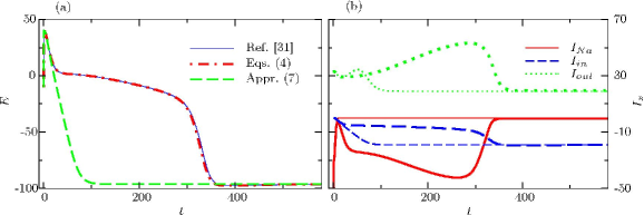
Figure 1: (Color online) (a) Action potential solutions of the original Noble model [32], equations (4), and of its “naive approximation”, equations (4) with (7). (b) Ionic currents ${I_{Na}}$ (solid red lines), ${I_{in}}$, (dashed blue lines) and ${I_{out}}$ (dotted green lines) in the model (4) (thick lines) and in the model (4) with (7) (thin lines). By the tradition accepted in physiology currents that increase voltage are considered negative and called “inward” and thus the three currents are defined as ${I_{Na}}\equiv{g_{Na}}\,{m^{3}_{\infty}}{{h}_{\infty}}\,\big{(}{E}-{{E}_{Na}}\big{)}$, ${I_{in}}\equiv{g_{Na_{1}}}\,\big{(}{E}-{{E}_{Na}}\big{)}$, ${I_{out}}\equiv\big{(}{g_{K}}\,n^{4}+{g_{K_{1}}}\big{)}({E}-{{E}_{K}})$. Notice that it is ${I_{Na}}$ rather than ${I_{in}}$ that is the main balance to ${I_{out}}$ in the full model (4) (thick lines), and there is no such balance for the naively simplified model (thin lines). These and all other solutions in the paper are calculated with initial conditions ${E}(0)=-10$, ${h}(0)=1$, ${n}(0)=0$ if not indicated otherwise.

2.2 Naive embedding

Seeking further simplification, we note that the functions ${m^{3}_{\infty}}({E})$ and ${{h}_{\infty}}({E})$ are approximately stepwise as illustrated in figure 2(a). Thus, as suggested in [9, 7], the crudest approximation of (4) is given by

$${m^{3}_{\infty}}({E})\approx{\theta}({E}-{{E}_{m}}),\qquad{{h}_{\infty}}({E})\approx{\theta}({{E}_{h}}-{E}),$$ (7)

where ${{E}_{m}}$, ${{E}_{h}}$ satisfy ${m^{3}_{\infty}}({{E}_{m}})=1/2$ and ${{h}_{\infty}}({{E}_{h}})=1/2$, respectively and ${\theta}(\cdot)$ is the Heaviside step function. A similar approximation was done in several earlier simplified models, e.g. [18, 17, 21]. They typically took, for simplicity, that ${{E}_{h}}={{E}_{m}}$. This however leads to unsatisfactory description of the front dissipation phenomenon [7].

The naive approximation (7) turns out to be unsuccessful as shown in figure 1(a). The AP produced when (7) is used does not have a plateau but returns immediately to the resting state. The reason for this behaviour is revealed by an analysis of the individual currents which are illustrated in figure 1(b) both for the detailed system (4) and for the approximation (7). In the detailed model, the sodium current remains significant during the plateau phase, successfully counteracting the potassium current for some time. In the approximated model, this current is virtually absent after the initial upstroke. This is due to the fact that during the slow decrease of the voltage, both the ${m}$ and ${h}$ gates remain close to their quasi-stationary values ${{m}_{\infty}}$, ${{h}_{\infty}}$, and their product ${W}({E})\equiv{m^{3}_{\infty}}{{h}_{\infty}}$ is exactly zero in the approximated model. In contrast, in the detailed model, this product remains significant and although it is much smaller than unity, when multiplied by the large factor ${g_{Na}}$, produces a sodium current which is comparable to the potassium and the leakage currents. The current ${W}({E})$ is called the “window” sodium current, because it runs in the region of voltages between ${{E}_{h}}$ and ${{E}_{m}}$ where the gates are supposed to be “almost closed” [4].

2.3 Axiomatic embedding

In this section we consider a more elaborate parametric embedding, the asymptotic limit of which dissects equations (4) into simpler subsystems. It is based on a number of observations of the properties of the Noble model, which will be discussed below, and may be formalized in the following

Axioms 1–7  The functions ${g_{Na}}$, ${f_{h}}({E})$, ${{h}_{\infty}}({E})$ and ${m^{3}_{\infty}}({E})$ are parametrically embedded in the functions $\underline{{{g_{Na}}}}({\epsilon})$, $\underline{{{f_{h}}}}({E};{\epsilon})$, $\underline{{{{h}_{\infty}}}}({E};{\epsilon})$ and $\underline{{{m^{3}_{\infty}}}}({E};{\epsilon})$, ${\epsilon}>0$, such that

• $\underline{{{g_{Na}}}}(\epsilon)={\epsilon}^{-1}{g_{Na}}$,

• $\underline{{{f_{h}}}}({E};{\epsilon})={\epsilon}^{-1}{f_{h}}({E})$,

• $\lim\limits_{{\epsilon}\rightarrow 0}\;\underline{{{m^{3}_{\infty}}}}({E};{\epsilon})={M}({E})\,{\theta}({E}-{{E}_{m}})$,
  where the function ${M}({E})$ is close to ${m^{3}_{\infty}}({E})$ for ${E}>{{E}_{m}}$,

• $\lim\limits_{{\epsilon}\rightarrow 0}\;\underline{{{{h}_{\infty}}}}({E};{\epsilon})={H}({E})\,{\theta}({{E}_{h}}-{E})$
  where the function ${H}({E})$ is close to ${{h}_{\infty}}({E})$ for ${E}<{{E}_{h}}$,

• ${{E}_{m}}>{{E}_{h}}$,

• $\lim\limits_{{\epsilon}\rightarrow 0}\;\left({\epsilon}^{-1}\underline{{{m^{3}_{\infty}}}}({E};{\epsilon})\,\underline{{{{h}_{\infty}}}}({E};{\epsilon})\right)\equiv{\tilde{W}}({E})>0$,
  where ${\tilde{W}}({E})$ is close to the window current ${W}({E})\equiv{m^{3}_{\infty}}({E}){{h}_{\infty}}({E})$,

• $\displaystyle\lim\limits_{{\epsilon}\rightarrow 0}\underline{{{S}}}({E};{\epsilon})\equiv\lim\limits_{{\epsilon}\rightarrow 0}\left(\underline{{{m^{3}_{\infty}}}}({E};{\epsilon})\frac{\partial}{\partial{E}}\underline{{{{h}_{\infty}}}}({E};{\epsilon})\right)=0$.

Indeed, the permittivity of the Na current ${g_{Na}}=400$ is large compared to those of the other currents ${g_{K}}=1.2$, $\max({g_{K_{1}}})=1.8$ and ${g_{Na_{1}}}=0.14$ and thus the values of associated small constants $g_{x}/{g_{Na}}$, $g_{x}={g_{K}},{g_{K_{1}}},{g_{Na_{1}}}$ are of the order of $10^{-2}$. This observation is formalized in Axiom I by an introduction of a small parameter ${\epsilon}$ which divides ${g_{Na}}$. Axiom II is postulated on the basis of the observation that the function ${f_{h}}({E})$ is large compared to ${f_{n}}({E})$ as illustrated in figure 2(b). These functions are reciprocal to the time-scale functions of the gates ${h}$ and ${n}$ and therefore ${h}$ is a fast variable while $n$ is slow. The speed of ${h}$ is even comparable to ${E}$ during the upstroke. These observations are justified in [9, 7], where we argued that although in healthy tissue ${E}$ can be, or at least seems, faster than ${h}$, there are important applications where the two variables should be considered of comparable speed. Axioms III (IV) are suggested by the fact that functions ${m^{3}_{\infty}}({E})$ (${{h}_{\infty}}({E})$) are close to $1$ above (below) some switch voltages ${{E}_{m}}$ (${{E}_{h}}$), and almost vanish otherwise as seen in figure 2(a). The two Axioms do not give a precise definition of the functions ${H}({E})$ and ${M}({E})$, they only require that these are reasonably close to ${{h}_{\infty}}({E})$ and ${m^{3}_{\infty}}({E})$ for those values of ${E}$ where these functions are not small. Here “reasonably close” means that replacement of ${{h}_{\infty}}({E})$ with ${H}({E})\,{\theta}({{E}_{h}}-{E})$ and ${m^{3}_{\infty}}({E})$ with ${M}({E})\,{\theta}({E}-{{E}_{m}})$ should not change significantly the properties of the solution. A possible choice for ${{E}_{m}}$ and ${{E}_{h}}$ is so that they satisfy ${m^{3}_{\infty}}({{E}_{m}})=1/2$ and ${{h}_{\infty}}({{E}_{h}})=1/2$. Axiom V is clearly satisfied for equations (4) as shown in figure 2(a). Some simplified models take ${{E}_{m}}={{E}_{h}}$ in similar situations [18, 21, 17], however we already know that such simplification affects the “front dissipation” feature of realistic models [7]. Axioms III–V have a corollary that

$$\lim\limits_{{\epsilon}\rightarrow 0}\left(\underline{{{m^{3}_{\infty}}}}({E};{\epsilon})\,\underline{{{{h}_{\infty}}}}({E};{\epsilon})\right)=0.$$ (8)

This indicates that the permittivity of the window current ${W}({E})$ is small of the order ${\epsilon}$. However, as discussed in subsection 2.2, it is a particular property of the Noble model that the window current is finite since it is multiplied by the large factor ${g_{Na}}$ which is of order ${\epsilon}^{-1}$. To ensure this we postulate Axiom VI. Finally, figure 2(b) demonstrates the plausibility of Axiom VII where the graph of the function ${S}({E})\equiv\underline{{{S}}}({E};1)$ is shown.

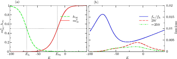
Figure 2: (Color online) Main functions of ${E}$ which determine the asymptotic properties of the model (4).

f:0020

Thus, according to Axioms I–VII the parametric embedding of the model (4) is

$$\frac{\mathrm{d}{E}}{\mathrm{d}{t}}={\epsilon}^{-1}{g_{1}}({E})\,\underline{{{m^{3}_{\infty}}}}({E};{\epsilon})\,{h}+{g_{2}}({E})\,{n}^{4}+{g_{3}}({E}),$$ (9a)

$$\frac{\mathrm{d}{h}}{\mathrm{d}{t}}={\epsilon}^{-1}{f_{h}}({E})\,\left(\underline{{{{h}_{\infty}}}}({E};{\epsilon})-{h}\right),$$ (9b)

$$\frac{\mathrm{d}{n}}{\mathrm{d}{t}}={f_{n}}({E})\,\left({{n}_{\infty}}({E})-{n}\right).$$ (9c)

First, we consider this system in the fast time ${T}={t}/{\epsilon}$. Changing the independent variable from ${t}$ to ${T}$, taking the limit ${\epsilon}\rightarrow 0$ and using Axioms III and IV, we obtain the fast-time system,

$$\begin{split}&\frac{\mathrm{d}{E}}{\mathrm{d}{T}}={g_{1}}({E})\,{M}({E})\,{\theta}({E}-{{E}_{m}})\,{h},\\ &\frac{\mathrm{d}{h}}{\mathrm{d}{T}}={f_{h}}({E})\,\left({H}({E})\,{\theta}({{E}_{h}}-{h})-{h}\right),\\ &\frac{\mathrm{d}{n}}{\mathrm{d}{T}}=0.\end{split}$$ (10)

As intended, the right-hand sides of the first two equations are nonzero, thus we have two fast variables, ${E}$ and ${h}$. The slow manifold is the set of equilibria of this system and it is defined by the finite equations

$${M}({E})\,{\theta}({E}-{{E}_{m}})\,{h}=0,$$ (11)

$${H}({E})\,{\theta}({{E}_{h}}-{E})-{h}=0,$$ (12)

since ${g_{1}}({E})>0$, ${f_{h}}({E})>0$ in the physiological range of the voltage, ${E}\in[{{E}_{K}},{{E}_{Na}}]$. Substitution of (12) into (11) with account of Axiom V turns (11) into an identity as the product of the two Heaviside functions vanishes. Thus, we have a codimension-1 slow manifold, defined by equation (12). This is a non-Tikhonov feature since in Tikhonov systems [30] the codimension of the slow manifold is equal to the number of fast variables. This peculiar feature results from (11) becoming an identity if (12) is satisfied, which, in turn, is due to a near-perfect switch behaviour of ${{h}_{\infty}}({E})$ and ${m^{3}_{\infty}}({E})$, becoming perfect switches in the limit ${\epsilon}\rightarrow 0$. A consequence of this feature is that the equilibria of the fast system are not isolated. Therefore, Tikhonov’s theorem [41] is not applicable as it requires asymptotic stability of equilibria of the fast system which does take place here. The fact that our parametric embedding is a non-Tikhonov one was already obvious from the dependence of (9) on the small parameter which is not of the form allowed by Tikhonov’s theorem, namely the large parameter ${\epsilon}^{-1}$ in the first equation multiplies only one of the terms in the right-hand side, rather than the whole right-hand side.

Since Tikhonov’s theorem cannot be used to describe the slow motion in the standard way, we discuss it in more detail, however without attempts of rigorous treatment. We consider system (9) in the original (slow) time, and restrict our attention to trajectories near the slow manifold, i.e. ones for which ${h}\approx\underline{{{{h}_{\infty}}}}({E};0)$. By re-arranging equation (9b), and assuming that when moving along the slow manifold the derivative $\mathrm{d}{{h}}/\mathrm{d}{{t}}$ is of order unity (this assumption is confirmed by the following result), we obtain

$${h}=\underline{{{{h}_{\infty}}}}({E};{\epsilon})-\frac{{\epsilon}}{{f_{h}}({E})}\frac{\mathrm{d}{h}}{\mathrm{d}{t}}=\underline{{{{h}_{\infty}}}}({E};{\epsilon})+O({\epsilon}).$$ (13)

From here we deduce that ${h}=\underline{{{{h}_{\infty}}}}({E};{\epsilon})+O({\epsilon})$. Differentiating this with respect to time and substituting the result back into the right-hand side of (13), we obtain

$${h}=\underline{{{{h}_{\infty}}}}({E};{\epsilon})-\frac{{\epsilon}}{{f_{h}}({E})}\,\frac{\partial\underline{{{{h}_{\infty}}}}}{\partial{E}}\frac{\mathrm{d}{E}}{\mathrm{d}{t}}+O({\epsilon}^{2}),$$ (14)

which substituted in equation (9a) yields

$$\frac{\mathrm{d}{E}}{\mathrm{d}{t}}={\epsilon}^{-1}{g_{1}}({E})\,\underline{{{m^{3}_{\infty}}}}({E};{\epsilon})\,\underline{{{{h}_{\infty}}}}({E};{\epsilon})-\frac{{g_{1}}({E})}{{f_{h}}({E})}\,\underline{{{S}}}({E};{\epsilon})\,\frac{\mathrm{d}{E}}{\mathrm{d}{t}}+O({\epsilon})+{g_{2}}({E})\,{n}^{4}+{g_{3}}({E}),$$ (15)

where the function $\underline{{{S}}}({E};{\epsilon})$ is defined in Axiom VII. Using Axiom VI for the first term and Axiom VII for the second term and taking the limit ${\epsilon}\rightarrow 0$ we obtain the slow-time system,

$$\begin{split}&\frac{\mathrm{d}{E}}{\mathrm{d}{t}}={g_{1}}({E})\,{\tilde{W}}({E})+{g_{2}}({E})\,{n}^{4}+{g_{3}}({E}),\\ &{h}={H}({E})\,{\theta}({{E}_{h}}-{E}),\\ &\frac{\mathrm{d}{n}}{\mathrm{d}{t}}={f_{n}}({E})\,\left({{n}_{\infty}}({E})-{n}\right).\end{split}$$ (16)

This is a system of two differential equations for the slow variables ${E}$ and ${n}$ plus a finite equation for ${h}$ defining the slow manifold. Note that we have two slow variables in agreement with the two dimensions of the slow manifold. Thus, ${E}$ is both a fast and a slow variable which is yet another non-Tikhonov feature.

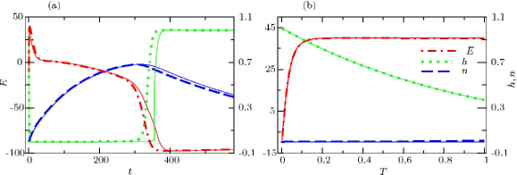
Figure 3: (Color online) Solution $({E},{h},{n})$ of the parametric embedding (9) with explicit expressions (17a) and (17b) with ${p}={q}=1$, ${r}=0.5$ for ${\epsilon}=1$ (thick lines, i.e. equivalent to the authentic model (4)) and ${\epsilon}=10^{-3}$ (corresponding thin solid lines) (a) in slow time ${t}\in[0,600]$, (b) in fast time ${T}\in[0,1]$.

f:0030

2.4 Explicit embedding

To show that Axioms I–VII are consistent and usable we need to demonstrate that there exist embedding functions $\underline{{{g_{Na}}}}$, $\underline{{{f_{h}}}}$, $\underline{{{{h}_{\infty}}}}$ and $\underline{{{m^{3}_{\infty}}}}$ which satisfy these axioms. The first two functions are already defined by Axioms I and II. Thus, in this section we suggest an explicit dependence of $\underline{{{m^{3}_{\infty}}}}$ and $\underline{{{{h}_{\infty}}}}$ on ${\epsilon}$ which satisfies Axioms III–VI, namely

$$\underline{{{m^{3}_{\infty}}}}({E};{\epsilon})\equiv{M}({E})\;\left({\epsilon}^{p}\,{\theta}({{E}_{h}}-{E})+{\epsilon}^{r}\,{\theta}({E}-{{E}_{h}})\,{\theta}({{E}_{m}}-{E})+{\theta}({E}-{{E}_{m}})\right),$$ (17a)

$$\underline{{{{h}_{\infty}}}}({E};{\epsilon})\equiv{H}({E})\;\left({\theta}({{E}_{h}}-{E})+{\epsilon}^{1-{r}}\,{\theta}({E}-{{E}_{h}})\,{\theta}({{E}_{m}}-{E})+{\epsilon}^{q}\,{\theta}({E}-{{E}_{m}})\right),$$ (17b)

where ${p}\in[1,+\infty)$, ${q}\in[1,+\infty)$, ${r}\in(0,1)$ and, of course, we must have ${M}({E})={m^{3}_{\infty}}({E})$, ${H}({E})={{h}_{\infty}}({E})$ to ensure these functions coincide with ${m^{3}_{\infty}}({E})$ and ${{h}_{\infty}}({E})$ at ${\epsilon}=1$. It straightforward to verify, that Axioms III–VI are then satisfied. To verify Axiom VII is more complicated: obviously, the above derivation of the slow system (16) is not technically valid for discontinuous $\underline{{{{h}_{\infty}}}}$ as defined by (17b), and Axiom VII does not make sense literally. Still, it will be satisfied if we assume that $\delta({E}-{{E}_{h}}){\theta}({E}-{{E}_{m}})=0$, i.e. infinity times zero at ${E}={{E}_{h}}$ equals zero. If ${p}={q}=1$, we have the asymptotic window current exactly equal to the window current of the Noble model, ${\tilde{W}}({E})={W}({E})$; if ${p}>1$ and ${q}>1$, then the asymptotic window current is a cut-off version of the original, ${\tilde{W}}({E})={W}({E})\,{\theta}({E}-{{E}_{h}})\,{\theta}({{E}_{m}}-{E})$. The adequacy of this embedding for ${p}={q}=1$, ${r}=0.5$ is demonstrated in figure 3.

The explicit embedding (17) is rather complicated. Formally, there are infinitely many embeddings; e.g. equations (17a) and (17b) define a three-parameter family of embeddings, all satisfying the Axioms and all leading to the same fast and slow systems and having the same asymptotic properties. And it is not possible to infer from the original problem, which of the embeddings is “correct”. The discontinuity of $\underline{{{{h}_{\infty}}}}$ and $\underline{{{m^{3}_{\infty}}}}$ is also a cause for concern. It is true that their limits in ${\epsilon}\rightarrow 0$ have to be discontinuous, or at least non-analytical, according to Axioms III and IV, but with (17a) and (17b) they are discontinuous already for any ${\epsilon}\neq 1$, which is inconvenient even in this heuristic treatment. Moreover, this is likely to cause serious technical difficulties in any attempt of rigorous treatment of the problem. This difficulty can be overcome, for instance, by using in (17a) and (17b), instead of Heaviside functions, functions which are smooth for all ${\epsilon}>0$ and only tend to Heaviside functions in the limit ${\epsilon}=0$, e.g.

$$\underline{{{\theta}}}(x;{\epsilon})=1/(1+e^{-x/{\epsilon}}).$$ (18)

Indeed, in that case the peak value of $\left|\partial\underline{{{{h}_{\infty}}}}({E};{\epsilon})/\partial{E}\right|$ is attained at ${E}={{E}_{h}}$ and is $(4{\epsilon})^{-1}{{h}_{\infty}}({{E}_{h}})$ in the leading order, whereas the value of $\underline{{{m^{3}_{\infty}}}}({{E}_{h}};{\epsilon})$ is exponentially small in ${\epsilon}$, thus their product is uniformly small and Axiom VII is satisfied.

3 The Archetypal Model

3.1 Formulation and parametric embedding

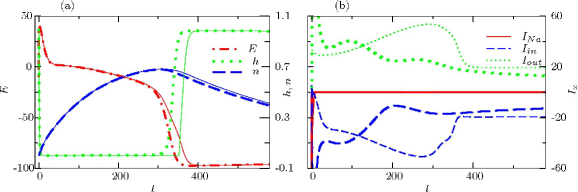
Figure 4: (Color online) (a) Solutions $({E},{h},{n})$ of the Noble model (4) (thick lines) and of the Archetypal Model (19) (corresponding thin solid lines). (b) Ionic currents ${I_{Na}}$ (solid red lines), ${I_{in}}$, (dashed blue lines) and ${I_{out}}$ (dotted green lines) in the model of Courtemanche et al. [15] (thick lines) and in the Archetypal Model (19) (thin lines). The ${I_{Na}}$-curves of the latter two models overlap. The definition of the currents is given in the caption of figure 1. Note that in both models, ${I_{out}}$ during the most of the AP is mainly balanced by ${I_{in}}$ but not ${I_{Na}}$.

f:0040

The complications arising in the construction of a possible embedding of the Noble model (4), as discussed in the preceding section, are not essential. In fact, they arise only due to the fact that insufficient experimental data was available at the time of the construction of the Noble model and in particular the existence of a Ca current was not yet discovered. Thus, the Na current was given a dual role to produce the upstroke and to keep voltage elevated during the long plateau stage leading to the large Na window illustrated in figure 1(b). Such a large window current is not present in other cardiac models. This is demonstrated in figure 4(b) in the case of the currently-accepted detailed ionic model of human atrial cells of Courtemanche et al. [15]. Bearing in mind the possibility of extending our present analysis and results to models of other types of cardiac cells, we propose a modified version of the Noble model (4). It is similar in many aspects to (4) in but has a more “generic cardiac” structure and admits a straightforward asymptotic embedding:

$$\begin{split}\frac{\mathrm{d}{E}}{\mathrm{d}{t}}&={g_{1}}({E})\,{M}({E})\,{\theta}({E}-{{E}_{m}})\,{h}+{g_{1}}({E})\,{W}({E})+{g_{2}}({E})\,{n}^{4}+{g_{3}}({E})\\ &={g_{1}}({E})\,{M}({E})\,{\theta}({E}-{{E}_{m}})\,{h}+{g_{2}}({E})\,{n}^{4}+{G}({E}),\\ \frac{\mathrm{d}{h}}{\mathrm{d}{t}}&={f_{h}}({E})\,\left({H}({E})\,{\theta}({{E}_{h}}-{E})-{h}\right),\\ \frac{\mathrm{d}{n}}{\mathrm{d}{t}}&={f_{n}}({E})\,\left({{n}_{\infty}}({E})-{n}\right),\end{split}$$ (19)

where the functions ${{m}_{\infty}}$, ${{h}_{\infty}}$, ${f_{h}}$, ${f_{n}}$, ${g_{1}}$, ${g_{2}}$, ${g_{3}}$ are defined as in equations (4), and ${M}({E})={m^{3}_{\infty}}({E}),$ ${H}({E})={{h}_{\infty}}({E}),$ ${G}({E})={g_{1}}({E}){W}({E})+{g_{3}}({E}),$ ${W}({E})={m^{3}_{\infty}}({E}){{h}_{\infty}}({E}).$ In this formulation, the perfect-switch behaviour of the Na gates is represented by the Heaviside functions multiplying ${M}$ and ${H}$. The deviation from the perfect-switch behaviour, due to the window current component ${W}={m^{3}_{\infty}}{{h}_{\infty}}$, is separated from the fast Na dynamics and appears as an additional “time-independent” current with a role similar to ${g_{3}}({E})$.

We shall call (19) the “Archetypal Model” (AM). The AP of this model is very similar to the AP of the Noble model (4) as shown in figure 4(a). Its simplest asymptotic embedding consistent with Axioms I–VII can be done with ${\epsilon}$ introduced linearly and only in two places,

$$\begin{split}&\frac{\mathrm{d}{E}}{\mathrm{d}{t}}={\epsilon}^{-1}{g_{1}}({E})\,{M}({E})\,{\theta}({E}-{{E}_{m}})\,{h}+{g_{1}}({E})\,{W}({E})+{g_{2}}({E})\,{n}^{4}+{g_{3}}({E}),\\ &\frac{\mathrm{d}{h}}{\mathrm{d}{t}}={\epsilon}^{-1}{f_{h}}({E})\,\left({H}({E})\,{\theta}({{E}_{h}}-{E})-{h}\right),\\ &\frac{\mathrm{d}{n}}{\mathrm{d}{t}}={f_{n}}({E})\,\left({{n}_{\infty}}({E})-{n}\right).\end{split}$$ (20)

The quality of this embedding is illustrated in figure 5. The limit of the fast-time system is

$$\begin{split}&\frac{\mathrm{d}{E}}{\mathrm{d}{T}}={g_{1}}({E})\,{M}({E})\,{\theta}({E}-{{E}_{m}})\,{h},\\ &\frac{\mathrm{d}{h}}{\mathrm{d}{T}}={f_{h}}({E})\,\left({H}({E})\,{\theta}({{E}_{h}}-{E})-{h}\right),\\ &\frac{\mathrm{d}{n}}{\mathrm{d}{T}}=0,\end{split}$$ (21)

and the limit of the slow-time system is

$$\frac{\mathrm{d}{E}}{\mathrm{d}{t}}={g_{1}}({E})\,{W}({E})+{g_{2}}({E})\,{n}^{4}+{g_{3}}({E}),$$ (22a)

$${h}={H}({E})\,{\theta}({{E}_{h}}-{E}),$$ (22b)

$$\frac{\mathrm{d}{n}}{\mathrm{d}{t}}={f_{n}}({E})\,\left({{n}_{\infty}}({E})-{n}\right).$$ (22c)

These systems coincide with (10) and (16), if ${\tilde{W}}({E})={W}({E})$. Their solutions and phase portraits are shown in figure 5 and figure 6, respectively.

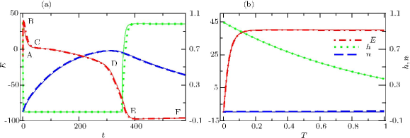
Figure 5: (Color online) Solution $({E},{h},{n}$) of the parametric embedding (20) for ${\epsilon}=1$ (thick lines, i.e. equivalent to the Archetypal Model (19)) and ${\epsilon}=10^{-3}$ (corresponding thin solid lines) (a) in slow time ${t}\in[0,600]$, (b) in fast time ${T}\in[0,1]$.

f:0050

The AM (19) produces an AP similar to the Noble model (4). In fact, the agreement between the two can be improved further as demonstrated in Appendix A. Moreover, the AM and the Noble model have the same asymptotic limits. The AM has two advantages. Firstly, the relevant asymptotic embedding is much simpler: the right-hand sides of (20) linearly depend on ${\epsilon}^{-1}$, and it appears only in two places. Secondly and more importantly, judging from figure 4(b), the asymptotic properties of the fast Na current in modern detailed models are likely to be similar to those of the AM (19) rather than to those of the Noble model (4). Therefore, we adopt the AM (19) as the example on which the non-Tikhonov asymptotic procedure is demonstrated.

3.2 Asymptotic analysis

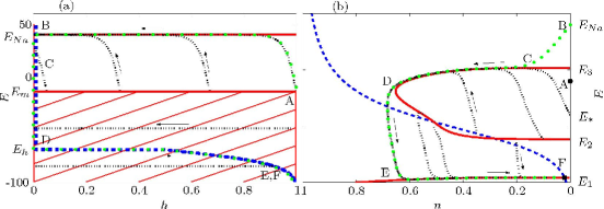
Figure 6: (Color online) Phase portraits of (a) the fast system (21) and (b) the slow system (22) of the Archetypal Model. Blue dashed lines represent vertical isoclines $\mathrm{d}{{h}}/\mathrm{d}{{t}}=0$ in (a) and $\mathrm{d}{{n}}/\mathrm{d}{{t}}=0$ in (b). Solid red lines and the cross-hatched region in (a) represent horizontal isoclines $\mathrm{d}{{E}}/\mathrm{d}{{t}}=0$. Thin dotted black lines with attched arrows represent trajectories. The thick dotted green line corresponds to the AP shown in figure 5(a). The letters A-F designate feature points of the solution. Notice that the blue set in (a) is a subset of the red set, so it is a continuous set of equilibria in the fast subsystem.

f:0060

3.2.1 The fast-time subsystem

The fast-time subsystem (21) of the AM governs the evolution of the two fast variables ${E}$ and ${h}$ on a time scale ${t}\sim{\epsilon}$ or equivalently ${T}\sim 1$. Its solution does not depend on the third variable ${n}$, which is slow and thus stays close to its initial value ${{n}_{0}}$ on this time scale.

System (21) admits exact analytical solution. If ${{E}_{0}}<{{E}_{m}}$ the solution of the initial-value problem with ${E}(0)={{E}_{0}}$, ${h}(0)={{h}_{0}}$ is

$$\begin{split}&{E}={{E}_{0}},\\ &{h}={H}({{E}_{0}})\,{\theta}({{E}_{h}}-{{E}_{0}})+\left({{h}_{0}}-{H}({{E}_{0}})\,{\theta}({{E}_{h}}-{{E}_{0}})\right)\,\exp\left(-{f_{h}}({{E}_{0}})\,{T}\right).\end{split}$$ (23)

If ${{E}_{0}}>{{E}_{m}}$ the solution of the same initial-value problem is given in quadratures by

$${h}={{h}_{0}}+{J}({{E}_{0}})-{J}({E}),$$ (24a)

$${T}=\int\limits_{{{E}_{0}}}^{{E}}\frac{\mathrm{d}{\eta}}{{g_{1}}({\eta})\,{M}({\eta})\,\left({{h}_{0}}+{J}({{E}_{0}})-{J}({\eta})\right)},$$ (24b)

where

$${J}({\eta})=\int\frac{{f_{h}}({\eta})}{{g_{1}}({\eta})\,{M}({\eta})}\,\mathrm{d}{{\eta}}.$$ (25)

Note that each trajectory of the fast-time subsystem (21) crosses the slow manifold (22b) only once as shown in figure 6(a). Thus, singularity of the slow manifold with respect to the trajectories of the fast system, which in Zeeman’s [46] interpretation of Tikhonov systems determines the threshold of excitation, does not exist in the AM. To shed light on the threshold properties of our fast-time subsystem, let us consider the maximal overshoot voltage ${{E}_{\infty}}\equiv{E}(+\infty)$ in the system as a function of the initial conditions. Taking into account that ${h}(+\infty)=0$ we can use (24a) to find ${{E}_{\infty}}$ as a solution of the finite equation ${J}\left({{E}_{\infty}}\right)={J}({{E}_{0}})+{{h}_{0}}$, provided that ${{E}_{0}}>{{E}_{m}}$ and, of course, ${{E}_{\infty}}={{E}_{0}}$, otherwise. Thus, the function ${{E}_{\infty}}({{E}_{0}},{{h}_{0}})$ has a discontinuity along the line $\{({{E}_{0}},{{h}_{0}})\}=\{{{E}_{m}}\}\times(0,1]$ as shown in figure 6(a). This discontinuity is the mathematical equivalent of the physiological notion of excitability: the upstroke does take place if and only if ${{E}_{0}}$ is above the threshold, ${{E}_{m}}$. Note that excitability in Tikhonov-Zeeman systems has this property, too, but is related to unstable branches of the slow manifold, rather than discontinuities in the fast flow.

The numerical values of parameters of the Noble model from which our Archetypal Model descends, are such that ${f_{h}}({E})/{g_{1}}({E})$ is a uniformly small function of ${E}$ in the physiological range. That is, condition ${{h}_{0}}={J}({{E}_{\infty}})-{J}({{E}_{0}})\sim 1$ requires relatively large values of the quadrature (25), the integrand of which is generally a relatively small quantity. This is achievable if the integration interval goes close to the pole of the integrand, i.e. zero of ${M}({\eta})$. In other words, the noted smallness of ${f_{h}}/{g_{1}}$ necessitates that ${{E}_{\infty}}\approx{{E}_{Na}}$ for typical ${{E}_{0}}$ and ${{h}_{0}}$. A more detailed and formal analysis of this aspect is given in Appendix B.

3.2.2 The slow-time subsystem

The slow-time subsystem (22) of the AM governs the evolution of the two slow variables ${E}$ and ${n}$ on a time scale ${t}\sim 1$ or ${T}\sim{\epsilon}^{-1}$. In fact, equations (22a) and (22c) form a closed subsystem. Gate ${h}$ described by (22b) can be evaluated if ${E}({t})$ is known but does not affect the dynamics of other variables. The slow-time system has been studied by Krinsky and Kokoz [28]. The slow-time subsystem (22) is, in turn, a fast-slow system, this time in the classical Tikhonov sense. This is illustrated by figure 7(a) which compares the characteristic time-scale functions of the dynamical variables ${E}$ and ${n}$, defined as $\tau_{y}=\left|\partial\dot{y}/\partial y\right|^{-1}$ for $y={E},{n}$. It can be seen that ${E}$ is a fast variable and ${n}$ is a slow variable, which motivates the introduction of a second small parameter ${\epsilon_{2}}>0$ in the following standard Tikhonov way,

$$\frac{\mathrm{d}{E}}{\mathrm{d}{t}}={G}({E})+{g_{2}}({E})\,{n}^{4},$$ (26a)

$$\frac{\mathrm{d}{n}}{\mathrm{d}{t}}={\epsilon_{2}}{f_{n}}({E})\,\left({{n}_{\infty}}({E})-{n}\right).$$ (26b)

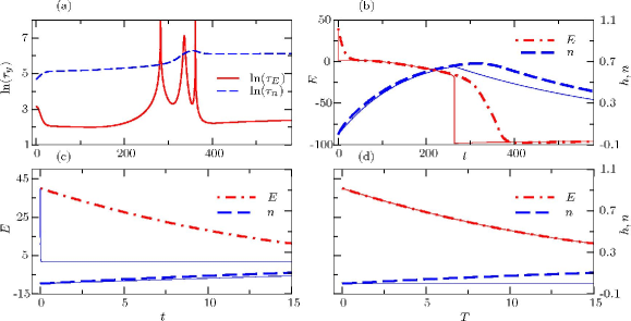
Figure 7: (Color online) (a) Characteristic time-scale functions $\tau_{y}=\left|\mathrm{d}\dot{y}/\mathrm{d}y\right|^{-1}$ for variables $y={E},{n}$ of the slow-time system (22) corresponding to the trajectory B-C-D-E-F in figure 5. (b – c) A solution $({E},{n}$) of the parametric embedding (26) for ${\epsilon_{2}}=1$ (thick lines, i.e. equivalent to the system (22)) and ${\epsilon_{2}}=10^{-3}$ (corresponding thin solid lines) (b) in slow time ${t}\in[0,600]$, (c) in slow time ${t}\in[0,15]$ and (d) in fast time ${T}\in[0,15]$.

f:0080

System (26) is a fast-time system. In the limit ${\epsilon_{2}}\rightarrow 0$ the lines ${n}={n}({{t}_{0}})=\mathrm{const}$ form the leaves of the fast foliation. On every such leaf the solution for the voltage is given by

$${t}-{{t}_{0}}=\int\limits_{{E}({{t}_{0}})}^{{E}({t})}\frac{\mathrm{d}{{\eta}}}{{G}({\eta})+{g_{2}}({\eta})\,{n}({{t}_{0}})^{4}}.$$ (27)

The corresponding slow-time system is obtained by the change of variable ${{t}_{2}}={\epsilon_{2}}{t}$ and in the limit ${\epsilon_{2}}\rightarrow 0$ becomes

$$0={G}({E})+{g_{2}}({E})\,{n}^{4},$$ (28a)

$$\frac{\mathrm{d}{n}}{\mathrm{d}{{t}_{2}}}={f_{n}}({E})\,\left({{n}_{\infty}}({E})-{n}\right).$$ (28b)

Equation (28a) defines the super-slow manifold,

$${n}={\mathcal{N}}({E})=\left(-{G}({E})/{g_{2}}({E})\right)^{1/4},$$ (29)

and equation (28b) describes the motion along this manifold. As illustrated in figure 6(b) the super-slow manifold is split into two parts by the condition ${n}^{4}\geq 0$: the “diastolic” branch ${E}\in(-\infty,{E_{1}}]$ and the “systolic” branch for ${E}\in[{E_{2}},{E_{3}}]$, where ${E_{1}}\approx-95.75$, ${E_{2}}\approx-61.81$ and ${E_{3}}\approx 1.86$ are roots of the equation ${G}({E})=0$. The stability of the fast equilibria is determined by the sign of $\partial\dot{{E}}/\partial{E}$ which coincides with the sign of ${\mathcal{N}}^{\prime}({E})=\mathrm{d}{{\mathcal{N}}}/\mathrm{d}{{E}}$: the stable branches of the super-slow manifold correspond to regions in $({n},{E})$ plane where its graph has a negative slope, i.e. ${\mathcal{N}}^{\prime}({E})<0$. These are the regions of the entire diastolic branch and the upper part of the systolic branch, corresponding to ${E}\in({E_{\ast}},{E_{3}}]$, where ${E_{\ast}}\approx-17.05$ is the root of the equation ${\mathcal{N}}^{\prime}({E_{\ast}})=0$. These considerations determine the excitability properties in terms of the super-slow subsystem (28). As seen in figure 6(b) the threshold of excitability is ${E_{2}}$ since a trajectory starting from $E({{t}_{0}})>{E_{2}}$ will be repelled by the lower systolic branch and attracted by the upper one, thus making a relatively large excursion. This will be followed by a slow movement along the upper systolic branch and a jump to the diastolic branch at ${E_{\ast}}$. On every monotonic branch of the super-slow manifold the equation (28a) can, in principle, be resolved with respect to ${E}$ to give ${E}={\mathcal{N}}^{-1}({n})$ and the result can be substituted into (28b) leading to the following quadrature solution of equations (28),

$$\begin{split}&{{t}_{2}}-{{{t}_{2}}_{,C}}=\int\limits_{{{n}_{C}}=0}^{{n}}\frac{\mathrm{d}{\nu}}{{f_{n}}\left({\mathcal{N}}^{-1}({\nu})\right)\,\left({{n}_{\infty}}\left({\mathcal{N}}^{-1}({\nu})\right)-{\nu}\right)},\\ &{E}={\mathcal{N}}^{-1}\left({n}({{t}_{2}})\right),\end{split}$$ (30)

where ${{{t}_{2}}_{,C}}$ is the slow time of the beginning of this asymptotic stage. Alternatively, we may use, as suggested in [32], ${E}$ rather than ${n}$ as a coordinate on the super-slow manifold. To do that we substitute ${n}={\mathcal{N}}({E})$ into the second equation

$$\frac{\mathrm{d}{E}}{\mathrm{d}{{t}_{2}}}=\frac{{f_{n}}({E})\,\left({{n}_{\infty}}({E})-{\mathcal{N}}({E})\right)}{{\mathcal{N}}^{\prime}({E})},$$

where from solution of the slow-time system in quadratures follows without the need to invert the function ${\mathcal{N}}({E})$. In particular, the time between the points $({E},{h})=({E_{3}},0)$ and $({E_{\ast}},{N_{\ast}})$, i.e. the duration of the plateau of an AP starting from ${n}=0$, is

$${{t}_{2}}({E_{\ast}})-{{t}_{2}}({E_{3}})=\int\limits_{{E_{3}}}^{{E_{\ast}}}\frac{{\mathcal{N}}^{\prime}({E})\,\mathrm{d}{{E}}}{{f_{n}}({E})\,\left({{n}_{\infty}}({E})-{\mathcal{N}}({E})\right)},$$ (31)

where ${N_{\ast}}={\mathcal{N}}({E_{\ast}})\approx 0.6512$ for the standard parameter values.

This completes a brief overview of the leading-order asymptotics of the Archetypal Model. An inventory of resulting formulas describing all the stages of typical solutions corresponding to various sorts of initial conditions, is given in Appendix C.

4 The caricature model

4.1 Motivation

As pointed out in the Introduction and throughout the article, the asymptotic structure of the embeddings of both the Noble and the Archetypal Model is non-Tikhonov and the results of the classical theory of slow-fast systems are not applicable. The fact that we are able to demonstrate a good numerical agreement in figures 3, 5 and 7 is reassuring but far from reliable since the numerical solutions are, by their nature, only approximate. Developing an alternative to the classical slow-fast asymptotic theory is beyond the scope ot this paper. Instead, in this section we propose and study a simple caricature model of cardiac excitation. One can think of the caricature model as a detailed ionic model which allows an exact solution and which has been embedded in a non-Tikhonov system. Once exact solutions are available, their the proximity to asymptotic solutions can be proved in this particular case. We have to emphasize that, the caricature is not “derived” from the Noble or from the Archetypal Model. They are, once again, used only as starting point for their simple functional forms. The caricature is constructed so that it has an asymptotic structure identical to that of the AM of section 3 and differs from it in that the functions in its the right-hand side are chosen so as to make possible to (a) evaluate the quadratures of section 3.2 and thus obtain explicit asymptotic solutions and (b) to go a step further and find an exact analytical solution of the simple model. We then proceed to to demonstrate that the appropriate limits of the exact analytical solution of this caricature model coincide with its solution in the asymptotic limits as given by quadratures (23), (24), (27), (30). Such an effort is still not a proof of our asymptotic analysis in general, but makes a good justification.

4.2 Formulation

In order to formulate a caricature of the AM (20) we keep the asymptotic structure of the latter and replace (“approximate”) the functions forming its right-hand side with simpler ones. We make the following simplifications.

1. We replace the functions ${M}({E})$ and ${H}({E})$ by unity. Thus, the function ${m^{3}_{\infty}}({E})$ is replaced by ${\theta}({E}-{{E}_{m}})$ and the function ${{h}_{\infty}}({E})$ by ${\theta}({{E}_{h}}-{E})$. Analogously, we replace the function ${{n}_{\infty}}({E})$ by ${\theta}({E}-{{E}_{n}})$. The values of the constants ${{E}_{m}}$, ${{E}_{h}}$ and ${{E}_{n}}$ will be discussed in item (e) below.

2. We replace the function ${f_{h}}({E})$ by the constant ${F_{h}}\equiv 1/2$. Analogously, we replace the function ${f_{n}}({E})$ by the constant ${F_{n}}\equiv 1/270$.

3. We replace the function ${G}({E})$ by the continuous piecewise linear function,

   $${\tilde{G}}({E})=\left\{\begin{array}[]{lll}{k_{1}}({E_{1}}-{E}),&{E}\in(-\infty,{E_{\dagger}}),\\ {k_{2}}({E}-{E_{2}}),&{E}\in[{E_{\dagger}},{E_{\ast}}),\\ {k_{3}}({E_{3}}-{E}),&{E}\in[{E_{\ast}},+\infty),\end{array}\right.$$ (32)

   where the constants ${k_{1}}\equiv 0.075$, ${k_{2}}\equiv 1/25$, ${k_{3}}\equiv 1/10$ while the constants ${E_{1}}\equiv-280/3$, ${E_{2}}\equiv-55$ and ${E_{3}}\equiv 1$ are close to the roots of ${G}({E})$ (which are $\approx-95.75$, $-61.81$ and $1.86$ respectively; we prefer to avoid multi-digit decimal values). The constants ${E_{\ast}}\equiv-15$ and ${E_{\dagger}}\equiv-80$ are determined by the intersection points of the three linear pieces of ${\tilde{G}}({E})$. Note that at ${E_{\ast}}$ the function ${\tilde{G}}({E})$ reaches its local maximum and thus ${E_{\ast}}$ corresponds to the point on the systolic branch of the super-slow manifold which forms the boundary between its stable and unstable parts.

4. We replace the function ${g_{2}}({E})$ by ${g_{2}^{0}}{\theta}({E}-{E_{\dagger}})$, where ${g_{2}^{0}}=-9$.

5. Finally, we set ${{E}_{m}}\equiv{E_{\ast}}$, ${{E}_{h}}={{E}_{n}}\equiv{E_{\dagger}}$. A more accurate approximation would be to choose these constants as the solutions of the equations ${m^{3}_{\infty}}({{E}_{m}})=1/2$, ${{h}_{\infty}}({{E}_{h}})=1/2$, and ${{n}_{\infty}}({{E}_{n}})=1/2$, respectively. However, this would lead to a caricature model, the right-hand side of which would consist of six pieces instead of only three as with the present choice. Obviously, this is not a principal difficulty but would be rather technically inconvenient. Moreover, the present choice preserves the relatively good quantitative agreement with the original models without the additional complications.

A justification for the simplifications of the functions ${m^{3}_{\infty}}({E})$ and ${{h}_{\infty}}({E})$ can be found in figure 2(a) while the rest of the replacements are illustrated in figure 8.

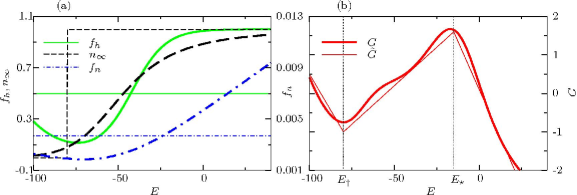
Figure 8: (Color online) (a – b) The caricature approximations (thin lines) of the right-hand side functions of the Archetypal Model (19) (thick lines).

f:0091

On these grounds, we postulate the following caricature of the AM (19),

$$\frac{\mathrm{d}{E}}{\mathrm{d}{t}}={\epsilon}^{-1}{G_{Na}}\,({{E}_{Na}}-{E})\,{\theta}({E}-{E_{\ast}})\,{h}+{g_{2}^{0}}{\theta}({E}-{E_{\dagger}})\,{n}^{4}+\tilde{{G}}({E}),$$ (33a)

$$\frac{\mathrm{d}{h}}{\mathrm{d}{t}}={\epsilon}^{-1}{F_{h}}\,\left({\theta}({E_{\dagger}}-{E})-{h}\right),$$ (33b)

$$\frac{\mathrm{d}{n}}{\mathrm{d}{t}}={\epsilon_{2}}\,{F_{n}}\,\left({\theta}({E}-{E_{\dagger}})-{n}\right),$$ (33c)

where we have included the artificial small parameters ${\epsilon}$ and ${\epsilon_{2}}$ to ensure the correct asymptotic structure of the system.

4.3 Exact solution

It is possible to obtain an exact analytical solution of the caricature model (33). Indeed, equations (33b) and (33c) are separable and simple enough to be easily solvable. After their solutions are substituted in equation (33a) it, too, becomes a readily-solvable first-order linear ODE. Therefore, assuming the initial conditions,

$${E}(0)={{E}_{0}}>{E_{\ast}},\quad{h}(0)=1,\quad{n}(0)=0,$$ (34)

of a fast-upstroke AP and natural continuity conditions at the ends of the three intervals separated by ${E_{\dagger}}$ and ${E_{\ast}}$ or, equivalently, at the ends of the corresponding time intervals ${t}\in[0,{{t}_{\ast}}]$, ${t}\in[{{t}_{\ast}},{{t}_{\dagger}}]$ and ${t}\in[{{t}_{\dagger}},\infty)$, system (33) has the following exact analytical solution,

$${n}({t})=\begin{cases}1-\exp(-{\epsilon_{2}}{F_{n}}{t}),&{t}\in[0,{{t}_{\dagger}}]\\[4.30554pt] \left(\exp({\epsilon_{2}}{F_{n}}{{t}_{\dagger}})-1\right)\exp(-{\epsilon_{2}}{F_{n}}{t}),&{t}\in[{{t}_{\dagger}},\infty]\end{cases}$$ (35a)

$${h}({t})=\begin{cases}\exp(-{F_{h}}{t}/{\epsilon}),&{t}\in[0,{{t}_{\dagger}}]\\[4.30554pt] 1-\left(1+\exp({F_{h}}{{t}_{\dagger}}/{\epsilon})\right)\exp(-{F_{h}}{t}/{\epsilon}),&{t}\in[{{t}_{\dagger}},\infty]\end{cases}$$ (35b)

$${E}({t})=\begin{cases}\displaystyle{\overset{1}{{E}}}({t})=\exp\Bigg{(}\frac{{G_{Na}}}{{F_{h}}}\,\exp\bigg{(}-\frac{{F_{h}}{t}}{{\epsilon}}\bigg{)}-{k_{3}}{t}\Bigg{)}\,\times&\\ \displaystyle\hskip 20.00003pt\Bigg{[}{{E}_{0}}\exp\bigg{(}-\frac{{G_{Na}}}{{F_{h}}}\bigg{)}-{k_{3}}{E_{3}}\,{u}(-{k_{3}},{t})&\\ \displaystyle\hskip 20.00003pt-{g_{2}^{0}}\sum\limits_{{l}=0}^{4}(-1)^{{l}}\,\dbinom{4}{{l}}\,{u}\left((4-{l})\,{\epsilon_{2}}{F_{n}}-{k_{3}},{t}\right)&\\ \displaystyle\hskip 20.00003pt-\frac{{G_{Na}}{{E}_{Na}}}{{\epsilon}}\,{u}\bigg{(}\frac{{F_{h}}}{{\epsilon}}-{k_{3}},{t}\bigg{)}\Bigg{]},&{t}\in[0,{t}_{*}]\\[2.15277pt] {\overset{2}{{E}}}({t})=\left({E_{\ast}}-{w}({{t}_{\ast}})\right)\,\exp\left({k_{2}}\,({t}-{{t}_{\ast}})\right)+{w}({t}),&{t}\in[{t}_{*},{{t}_{\dagger}}]\\[4.30554pt] {\overset{3}{{E}}}({t})=({E_{\dagger}}-{E_{1}})\exp\left(-{k_{1}}({t}-{{t}_{\dagger}})\right)+{E_{1}},&{t}\in[{{t}_{\dagger}},\infty]\end{cases}$$ (35c)

where

$${u}({\varkappa},{t})\equiv\frac{{\epsilon}}{{F_{h}}}\bigg{(}\frac{{G_{Na}}}{{F_{h}}}\bigg{)}^{-\frac{{\varkappa}{\epsilon}}{{F_{h}}}}\Bigg{[}\Gamma\Bigg{(}\frac{{\varkappa}{\epsilon}}{{F_{h}}},\frac{{G_{Na}}}{{F_{h}}}\Bigg{)}-\Gamma\Bigg{(}\frac{{\varkappa}{\epsilon}}{{F_{h}}},\frac{{G_{Na}}}{{F_{h}}}\,\exp\bigg{(}{-\frac{{F_{h}}{t}}{{\epsilon}}}\bigg{)}\Bigg{)}\Bigg{]},$$ (36a)

$${w}({t})\equiv{E_{2}}-{g_{2}^{0}}\sum\limits_{{l}=0}^{4}(-1)^{{l}}\dbinom{4}{{l}}\frac{\exp\left(-{l}\,{\epsilon_{2}}{F_{n}}{t}\right)}{{k_{2}}+{l}\,{\epsilon_{2}}{F_{n}}},$$ (36b)

and $\Gamma(a,x)$ is the upper incomplete gamma function, $\Gamma(a,x)\equiv\int_{x}^{\infty}z^{a-1}e^{-z}\,\mathrm{d}{z}$ for $\mathrm{Re}(a)>0$ and $\Gamma(a+1,x)=a\Gamma(a,x)+x^{a}\,e^{-x}$ as defined in [2]. The exact analytical solution is plotted in figure 9 where it is compared with the numerical solutions of the AM (19) and the internal boundary points ${E_{\dagger}}$ and ${E_{\ast}}$ are also indicated. The parameters ${{t}_{\ast}}$ and ${{t}_{\dagger}}$ can be found as solutions of

$${\overset{1}{{E}}}({{t}_{\ast}})={E_{\ast}},\qquad{\overset{2}{{E}}}({{t}_{\dagger}})={E_{\dagger}}.$$ (37)

Both equations are transcendental and not solvable analytically. It is possible to solve them by using perturbation expansions about the small parameters ${\epsilon}$ and ${\epsilon_{2}}$. This, however, will contribute little beyond its value as a technical exercise and will lead us away from the main point of this part, which is to validate the asymptotic solutions for ${E}({t})$, ${h}({t})$ and ${n}({t})$. So here we omit these formulae, assuming that ${{t}_{\ast}}$ and ${{t}_{\dagger}}$ are known where they are needed. Numerically, for the standard values of parameters and ${{E}_{0}}=-10$, we obtain ${{t}_{\ast}}\approx 292.815$ and ${{t}_{\dagger}}\approx 345.241$.

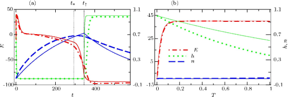
Figure 9: (Color online) The numerical solution of the embedding of the Archetypal Model (20) (thick lines) in comparison with the analytical solution (35) of the caricature model (33) (corresponding thin lines) (a) in slow time ${t}\in[0,600]$, for ${\epsilon}=1$, ${\epsilon_{2}}=1$, and (b) in fast time ${T}\in[0,1]$, for ${\epsilon}=10^{-3}$, ${\epsilon_{2}}=10^{-3}$.

f:0092

5 Validation of the general asymptotic analysis

In the following we consider the stages of a normal fast-upstroke AP. For each stage we (a) evaluate the appropriate quadratures of section 3.2 to obtain explicit asymptotic solutions for this stage and (b) evaluate the limit of the exact analytical solution (35) as the small parameters tend to zero as appropriate for the same stage. The asymptotic theory will be validated if the results from these two steps are identical.

5.1 Fast upstroke, stage A–B

Here and below, letters A–F refer to the labels in figure 5(a). The fast upstroke occurs during the interval ${t}\in[0,{{t}_{B}}]\subset[0,{{t}_{\ast}}]$, where ${{t}_{B}}\to 0$ but ${{t}_{B}}/{\epsilon}\to\infty$ as ${\epsilon}\to 0$. During this stage ${E}$ and the $h$-gate change together on a time scale $\sim{\epsilon}$ from the point $({E},{h})=({{E}_{0}},1)$ to $({{E}_{B}},0)$ while ${n}$ is a slow variable and remains approximately at its initial value ${n}\approx{{n}_{0}}=0$.

(a) Asymptotic solution. Asymptotically, this stage is described by quadratures (24,25). Substituting there the functions defined in section 4.2, we obtain

$${h}({E})=1+\frac{{F_{h}}}{{G_{Na}}}\,\ln\left(\frac{{{E}_{Na}}-{E}}{{{E}_{Na}}-{{E}_{0}}}\right),$$ (38a)

$${T}({E})=-\frac{1}{{F_{h}}}\,\ln\Bigg{(}1+\frac{{F_{h}}}{{G_{Na}}}\,\ln\left(\frac{{{E}_{Na}}-{E}}{{{E}_{Na}}-{{E}_{0}}}\right)\Bigg{)}.$$ (38b)

Solving (38b) for the voltage ${E}$ and substituting the result in (38a), we arrive at an explicit asymptotic solution,

$$\begin{split}&{E}={{E}_{Na}}-({{E}_{Na}}-{{E}_{0}})\,\exp\left(\frac{{G_{Na}}}{{F_{h}}}\left(e^{-{F_{h}}{T}}-1\right)\right),\\ &{h}=e^{-{F_{h}}{T}}.\end{split}$$ (39)

The maximal overshoot voltage ${{E}_{B}}$ is obtained as the fast time ${T}$ tends to infinity,

$${{E}_{B}}={{E}_{\infty}}=\lim\limits_{{T}\rightarrow+\infty}{E}({T})={{E}_{Na}}-({{E}_{Na}}-{{E}_{0}})\,\exp\left(-\frac{{G_{Na}}}{{F_{h}}}\right).$$ (40)

Since $\exp(-{G_{Na}}/{F_{h}})\approx 10^{-29}$, the maximal overshoot voltage ${{E}_{B}}$ is extremely close to ${{E}_{Na}}$ and ${h}({{t}_{B}})={h}({T}\to\infty)=0$ as expected.

(b) Limit of the exact solution. We change to fast time, ${T}={t}/{\epsilon}$, and take the limit of (35b) and (35c) as ${\epsilon}$ tends to zero, for fixed ${T}$. Since $\lim\limits_{a\to 1}\Gamma(a,x)=\exp(-x)$, it follows that $\lim\limits_{{\epsilon}\to 0}{u}({\varkappa},{\epsilon}{T})=0$, for ${\varkappa}\sim 1$ and therefore

$$\lim_{{\epsilon}\to 0}{u}(-{k_{3}},{\epsilon}{T})=0,$$

$$\lim_{{\epsilon}\to 0}{u}\left((4-{l})\,{\epsilon_{2}}{F_{n}}-{k_{3}},{\epsilon}{T}\right)=0.$$

Further,

$${u}\left(\frac{{F_{h}}}{{\epsilon}}-{k_{3}},{\epsilon}{T}\right)\approx\frac{{\epsilon}}{{G_{Na}}}\left[\exp\left(-\frac{{G_{Na}}}{{F_{h}}}\right)-\exp\left(-\frac{{G_{Na}}}{{F_{h}}}e^{-{F_{h}}{T}}\right)\right].$$

Therefore, taking the limit ${\epsilon}\to 0$ of expression ${\overset{1}{{E}}}$ in (35c) we obtain,

$$\begin{split}&\lim\limits_{{\epsilon}\to 0}{E}({\epsilon}{T})={{E}_{Na}}-({{E}_{Na}}-{{E}_{0}})\,\exp\left(\frac{{G_{Na}}}{{F_{h}}}\left(e^{-{F_{h}}{T}}-1\right)\right),\\ &\lim\limits_{{\epsilon}\to 0}{h}({\epsilon}{T})=e^{-{F_{h}}{T}}.\end{split}$$ (41)

Since equations (39) and (41) are identical, the asymptotic theory of the fast upstroke of the AP is validated.

5.2 Post-overshoot drop of the voltage, stage B–C

This corresponds to the time interval ${t}\in[{{t}_{B}},{{t}_{C}}]\subset[0,{{t}_{\ast}}]$, where ${{t}_{C}}\to+\infty$ but ${\epsilon_{2}}{{t}_{C}}\to 0$ as ${\epsilon_{2}}\to 0$. We keep ${{t}_{B}}$ in some of the formulae rather than replacing it with its limit, $\lim_{{\epsilon}\to 0}{{t}_{B}}=0$, as a symbolic reminder of the beginning of this asymptotic stage. The voltage ${E}$ decreases on a time scale $\sim 1$ towards the stable systolic branch, the ${h}$-gate remains at ${h}\approx 0$ and the slow ${n}$-gate also remains approximately unchanged at ${n}\approx{{n}_{0}}=0$.

(a) Asymptotic solution. The asymptotics of this stage are given by quadrature (27) which, with account of the approximations of section 4.2 and of the fact that asymptotically ${n}=0$, evaluates to

$${t}-{{t}_{B}}=\frac{1}{{k_{3}}}\,\ln\left(\frac{{E_{3}}-{{E}_{B}}}{{E_{3}}-{E}}\right).$$ (42)

Solving for ${E}({t})$, the explicit asymptotic solution for this stage is,

$${E}({t})={E_{3}}+({{E}_{B}}-{E_{3}})e^{-{k_{3}}({t}-{{t}_{B}})}.$$ (43)

(b) Limit of the exact solution. We are still within the interval ${t}\in[{{t}_{B}},{{t}_{C}}]\subset[0,{{t}_{\ast}}]$ and so use ${\overset{1}{{E}}}({t})$ of (35c). Taking the limit of (35a) and (35b) as ${\epsilon}$ and ${\epsilon_{2}}$ tend to zero, we obtain

$$\lim\limits_{{\epsilon_{2}}\to 0}{n}({t})=0,$$ (44a)

$$\lim\limits_{{\epsilon}\to 0}{h}({t})=0,$$ (44b)

in agreement with the asymptotic analysis.

Now we consider the limit of ${\overset{1}{{E}}}({t})$ given by (35c) for ${\epsilon}\to 0$ and ${\epsilon_{2}}\to 0$ at a fixed ${t}\in(0,{{t}_{\ast}})$. In the limit ${\epsilon_{2}}\to 0$ the terms ${u}\left((4-{l})\,{\epsilon_{2}}{F_{n}}-{k_{3}},{t}\right)$ become independent of the index ${l}$ and the sum over ${l}$ in the expression for ${\overset{1}{{E}}}({t})$ vanishes since the binomial coefficients cancel each other. For the remaining upper incomplete gamma functions, we use the recurrence relation,

$$\Gamma(a+1,x)=a\,\Gamma(a,x)+x^{a}\,e^{-x}$$

and the following asymptotics in the limit $a\searrow 0$,

$$\begin{split}&\Gamma(-a,x)=\mbox{Ei}(1,x)+O(a),\\ &\Gamma\left(-a,A\exp(-B/a)\right)=-a^{-1}\left(1-e^{B}\right)+O(1),\end{split}$$ (45)

for fixed $x,A,B>0$ and where $\mbox{Ei}(\nu,x)=\int_{1}^{\infty}z^{-\nu}\exp(-xz)\,\mathrm{d}{z}$, $\mathrm{Re}(x)>0$ is the exponential integral. Hence, as ${\epsilon}\to 0$, we have

$${u}(-{k_{3}},{t})\approx{k_{3}}^{-1}\left(1-e^{{k_{3}}{t}}\right),$$ (46)

$${u}\left(\frac{{F_{h}}}{{\epsilon}}-{k_{3}},{t}\right)\approx\frac{{\epsilon}}{{G_{Na}}}\Bigg{(}\exp\bigg{(}-\frac{{G_{Na}}}{{F_{h}}}\bigg{)}-1\Bigg{)}.$$ (47)

Substituting these results into the expression for ${\overset{1}{{E}}}$ in (35c) and taking the limits ${\epsilon}\to 0$ and ${\epsilon_{2}}\to 0$, we get

$$\lim_{{\epsilon_{2}},{\epsilon}\to 0}{\overset{1}{{E}}}(t)={E_{3}}+\Bigg{(}{{E}_{Na}}-({{E}_{Na}}-{{E}_{0}})\exp\bigg{(}-\frac{{G_{Na}}}{{F_{h}}}\bigg{)}-{E_{3}}\Bigg{)}e^{-{k_{3}}{t}},$$ (48)

which with account of (40), coincides with the asymptotic expression (43) where ${{t}_{B}}$ is taken at its limit, ${{t}_{B}}=0$. Thus the asymptotic procedure is validated in this stage as well.

5.3 Plateau, stage C–D

This corresponds to the time interval ${t}\in[{{t}_{C}},{{t}_{D}}]\subset[0,{{t}_{\ast}}]$. Again, we keep ${{t}_{C}}$ in some formulae as a symbolic reminder of the beginning of this asymptotic stage, $1\ll{{t}_{C}}\ll{\epsilon_{2}}^{-1}$, and we define ${{t}_{D}}={{t}_{\ast}}$ precisely. The voltage ${E}$ and the ${n}$-gate change on a time scale of the order ${{t}_{D}}-{{t}_{C}}=O({\epsilon_{2}}^{-1})$ along the upper systolic branch of the super-slow manifold until ${E}({{t}_{\ast}})={E_{\ast}}$ and ${n}({{t}_{\ast}})\approx{N_{\ast}}$. The ${h}$-gate remains close to its quasi-stationary value at ${h}\approx 0$.

(a) Asymptotic solution. The general asymptotic results describing this stage are given by (30). Since the functions of the caricature model in the time interval ${t}\in[0,{{t}_{\ast}}]$ are ${\tilde{G}}({E})={k_{3}}({E_{3}}-{E})$, ${{n}_{\infty}}({E})=1$, ${g_{2}}({E})={g_{2}^{0}}$, ${f_{n}}({E})={F_{n}}$, the quadrature (30) evaluates to

$${n}=1-\exp\left(-{F_{n}}({{t}_{2}}-{{{t}_{2}}_{,C}})\right),$$ (49a)

$${E}={E_{3}}+\frac{{g_{2}^{0}}}{{k_{3}}}\left(1-\exp\left(-{F_{n}}({{t}_{2}}-{{{t}_{2}}_{,C}})\right)\right)^{4},$$ (49b)

where ${{{t}_{2}}_{,C}}={\epsilon_{2}}{{t}_{C}}$ and $\lim\limits_{{\epsilon_{2}}\to 0}{{{t}_{2}}_{,C}}=0$.

(b) Limit of the exact solution. The plateau stage occurs during the time interval ${t}\in[0,{{t}_{\ast}}]$. In order to compare the limit of the exact solution (35) to equations (49) we need to change to the super-slow time, ${{t}_{2}}={\epsilon_{2}}{t}$. Then the solution (35a) for ${n}({{t}_{2}})$ does not contain a small parameter and is readily comparable with the asymptotics,

$$\lim\limits_{{\epsilon_{2}}\to 0}{n}({{t}_{2}})=1-\exp\left(-{F_{n}}({{t}_{2}}-{{{t}_{2}}_{,C}})\right),$$ (50)

where we have taken into account that the initial value of ${n}$ according to (44a) is ${n}({{{t}_{2}}_{,C}})=0$.

For the voltage during this stage, we consider ${\overset{1}{{E}}}$ from (35c) with a change to the super-slow time ${{t}_{2}}={\epsilon_{2}}{t}$,

$$\begin{split}\displaystyle{\overset{1}{{E}}}({\epsilon_{2}}^{-1}{{t}_{2}})=&{{E}_{\mathrm{BC}}}({\epsilon_{2}}^{-1}{{t}_{2}})\\ \displaystyle&+\exp\Bigg{(}\frac{{G_{Na}}}{{F_{h}}}\,\exp\bigg{(}-\frac{{F_{h}}{{t}_{2}}}{{\epsilon}\,{\epsilon_{2}}}\bigg{)}-\frac{{k_{3}}{{t}_{2}}}{{\epsilon_{2}}}\Bigg{)}\,{g_{2}^{0}}\sum\limits_{{l}=0}^{4}(-1)^{l}\,\dbinom{4}{{l}}\,{u}\left((4-{l})\,{\epsilon_{2}}{F_{n}}-{k_{3}},\frac{{{t}_{2}}}{{\epsilon_{2}}}\right),\end{split}$$ (51)

and look for the limit ${\epsilon}\to 0$, ${\epsilon_{2}}\to 0$ at a fixed ${{t}_{2}}$. The terms denoted here by ${{E}_{\mathrm{BC}}}({\epsilon_{2}}^{-1}{{t}_{2}})$ are precisely those discussed in connection with the limit of the exact solution during stage B–C with the only difference that now we consider them in the super-slow time ${{t}_{2}}$. For a fixed ${{t}_{2}}$, and small ${\epsilon_{2}}$, expression (48) evaluates to

$$\lim_{{\epsilon_{2}}\to 0}{{E}_{\mathrm{BC}}}({\epsilon_{2}}^{-1}{{t}_{2}})={E_{3}}.$$ (52)

Using expressions (45) derived in the previous stage the remaining ${u}(\cdot,\cdot)$-function in (51) in the limit ${\epsilon}\to 0$ becomes

$$\lim_{{\epsilon}\to 0}{u}\left((4-{l})\,{\epsilon_{2}}{F_{n}}-{k_{3}},\frac{{{t}_{2}}}{{\epsilon_{2}}}\right)=-\frac{1-\exp\left({k_{3}}{{t}_{2}}\right)\,\exp\left(-(4-{l}){F_{n}}{{t}_{2}}\right)}{(4-{l})\,{\epsilon_{2}}{F_{n}}-{k_{3}}}.$$ (53)

The exponentially growing term is cancelled by $\exp(-{k_{3}}{{t}_{2}}/{\epsilon_{2}})$ in (51) and therefore substituting the above expressions in (51) and taking the limit ${\epsilon_{2}}\to 0$ ultimately gives

$$\displaystyle\lim_{{\epsilon_{2}},{\epsilon}\to 0}{\overset{1}{{E}}}({{t}_{2}})={E_{3}}+\frac{{g_{2}^{0}}}{{k_{3}}}\left(1-\exp(-{F_{n}}{{t}_{2}})\right)^{4},$$ (54)

in full accord with the asymptotic result (49b) for the plateau stage of the AP, if we replace ${{{t}_{2}}_{,C}}$ with its limit $\lim\limits_{{\epsilon_{2}}\to 0}{{{t}_{2}}_{,C}}=0$.

Before proceeding to the next stage, we comment on the position of the point D on the $({n},{E})$ plane, which is close to the end of the systolic branch of the super-slow manifold, the point $({N_{\ast}},{E_{\ast}})$. As stated earlier, we define point D by the exact condition ${E}({{t}_{\ast}})={E_{\ast}}$, hence the condition ${n}({{t}_{\ast}})\approx{N_{\ast}}$ is only approximate, since the AP trajectory follows the super-slow manifold only approximately, with precision $O({\epsilon_{2}})$. We shall see shortly that for the next stage it is important that ${n}({{t}_{\ast}})\neq{N_{\ast}}$. The sense of this inequality can be easily seen from (26a): we know that during the C–D stage ${E}({t})$ decreases, ${G}({E})>0$ and ${g_{2}}({E})<0$, hence ${n}>\left(-{G}({E})/{g_{2}}({E})\right)^{1/4}={\mathcal{N}}({E})$ during the whole of that stage, which for ${t}={{t}_{\ast}}$, ${E}={E_{\ast}}$ gives ${n}>{\mathcal{N}}({E_{\ast}})={N_{\ast}}$. More accurately the value of ${n}({{t}_{\ast}})$ can be estimated using perturbation theory in ${\epsilon_{2}}$ around the super-slow manifold ${n}={\mathcal{N}}({E})$; this would be a further distraction from our main goal, and we omit these formulae, like in the problem of determining ${{t}_{\ast}}$ and ${{t}_{\dagger}}$.

5.4 Repolarization, stage D–E

During this stage the voltage ${E}$ jumps on a time scale $\sim 1$ from the systolic to the diastolic branch of the super-slow manifold. The ${h}$-gate changes swiftly on a time scale $\sim{\epsilon}$ from its lower quasi-stationary value close to zero to its upper quasi-stationary value close to unity due to the discontinuity in the right-hand side of equation (33b). The slow ${n}$-gate remains approximately unchanged at ${n}\approx{N_{\ast}}$. The associated time interval is ${t}\in[{{t}_{D}},{{t}_{E}}]=[{{t}_{\ast}},{{t}_{\dagger}}]\cup[{{t}_{\dagger}},{{t}_{E}}]$ where ${{t}_{D}}={{t}_{\ast}}$ is the beginning of this stage, ${{t}_{\dagger}}$ is the time of the inflexion point defined by ${E}({{t}_{\dagger}})={E_{\dagger}}$ and ${{t}_{E}}$ is the time of the end of the stage constrained by $1\ll{{t}_{E}}-{{t}_{\dagger}}\ll{\epsilon_{2}}^{-1}$.

(a) Asymptotic solution. The asymptotics at this stage are given by quadrature (27). During this stage of the AP, the form of the caricature equations changes as the solution ${E}({t})$ moves through the point ${E_{\dagger}}$.

In the time interval ${t}\in[{{t}_{\ast}},{{t}_{\dagger}}]$ the relevant functions of the caricature model are ${\tilde{G}}({E})={k_{2}}({E}-{E_{2}})$ and ${g_{2}}({E})={g_{2}^{0}}$ and therefore quadrature (27) evaluates to

$${E}=\left({E_{2}}-\frac{{g_{2}^{0}}{n}({{t}_{\ast}})^{4}}{{k_{2}}}\right)+\Bigg{(}{E_{\ast}}-\left({E_{2}}-\frac{{g_{2}^{0}}{n}({{t}_{\ast}})^{4}}{{k_{2}}}\right)\Bigg{)}\exp\left({k_{2}}({t}-{{t}_{\ast}})\right),$$ (55a)

$${n}={n}({{t}_{\ast}})=1-\exp{\left(-{F_{n}}({{{t}_{2}}_{,\ast}}-{{{t}_{2}}_{,C}})\right)}=\mathrm{const},$$ (55b)

with initial conditions ${n}({{t}_{\ast}})$ and ${E}({{t}_{\ast}})\equiv{E_{\ast}}$. The function ${E}({t})$ given by expression (55a) monotonically decreases since ${n}({{t}_{\ast}})>{N_{\ast}}=({k_{2}}({E_{\ast}}-{E_{2}})/{g_{2}^{0}})^{1/4}$. In the second time interval, ${t}\geq{{t}_{\dagger}}$, the relevant functions of the caricature model are ${\tilde{G}}({E})={k_{1}}({E_{1}}-{E})$ and ${g_{2}}({E})=0$, and quadrature (27) gives

$$\begin{split}&{E}({t})=({E_{\dagger}}-{E_{1}})\exp\left(-{k_{1}}({t}-{{t}_{\dagger}})\right)+{E_{1}},\\ &{n}({t})={n}({{t}_{\ast}})=\mathrm{const},\end{split}$$ (56)

with initial conditions ${n}({{t}_{\ast}})$ and ${E}({{t}_{\dagger}})={E_{\dagger}}$.

Finally, we note that the dynamics of ${h}$ gate during this stage have a peculiarity due to the discontinuity of the right-hand side of (33b). The finite constraint ${h}={\theta}({E_{\dagger}}-{E})$ which according to (22b) is supposed to be approximately observed outside the AP upstroke, cannot be observed when ${E}$ crosses the level ${E_{\dagger}}$, as this would mean a discontinuity in ${h}({t})$. In fact, the jump of ${h}({t})$ from 1 to 0 happens gradually, of course. We can see from (33b) that this jump takes time $\sim{\epsilon}$. This violation of (22b) does not, however, in any way affect the dynamics of ${E}$ and ${n}$, as ${{E}_{h}}={E_{\dagger}}<{{E}_{m}}={E_{\ast}}$ and therefore the factor ${h}\,{\theta}({E}-{E_{\ast}})$ in (33a) remains identically zero throughout this stage.

(b) Limit of the exact solution. In order to compare the asymptotic and the exact solutions in a given AP stage we need to align them in time. The beginning of the present stage is ${{t}_{D}}={{t}_{\ast}}={{{t}_{2}}_{,\ast}}/{\epsilon_{2}}$, so we set

$${t}={\epsilon_{2}}^{-1}{{{t}_{2}}_{,\ast}}+{\tilde{{t}}}$$ (57)

and then consider the limit ${\epsilon},{\epsilon_{2}}\to 0$ at a fixed ${\tilde{{t}}}$. As discussed earlier, we assume here that the limit of ${{{t}_{2}}_{,\ast}}$ is known (and finite). With this the exact solution in the interval ${t}\in[{{t}_{\ast}},{{t}_{\dagger}}]$ becomes

$${n}({\epsilon_{2}}^{-1}{{{t}_{2}}_{,\ast}}+{\tilde{{t}}})=1-\exp(-{F_{n}}{{{t}_{2}}_{,\ast}}-{\epsilon_{2}}{F_{n}}{\tilde{{t}}}),$$ (58a)

$${\overset{2}{{E}}}({\epsilon_{2}}^{-1}{{{t}_{2}}_{,\ast}}+{\tilde{{t}}})=\left({E_{\ast}}-{w}({\epsilon_{2}}^{-1}{{{t}_{2}}_{,\ast}})\right)\,\exp\left({k_{2}}\,{\tilde{{t}}}\right)+{w}({\epsilon_{2}}^{-1}{{{t}_{2}}_{,\ast}}+{\tilde{{t}}}).$$ (58b)

We have immediately that in the limit ${\epsilon_{2}}\to 0$, expression (58a) coincides with (55b), since $\lim{{{t}_{2}}_{,C}}=0$. Then, we have from (36b)

$$\lim\limits_{{\epsilon_{2}}\to 0}{w}\left(\frac{{{{t}_{2}}_{,\ast}}}{{\epsilon_{2}}}+{\tilde{{t}}}\right)={E_{2}}-\frac{{g_{2}^{0}}}{{k_{2}}}\,\sum\limits_{{l}=0}^{4}(-1)^{{l}}\,\dbinom{4}{{l}}\,e^{-{l}{F_{n}}{{{t}_{2}}_{,\ast}}}={E_{2}}-\frac{{g_{2}^{0}}}{{k_{2}}}\left(1-\exp(-{F_{n}}{{{t}_{2}}_{,\ast}})\right).$$ (59)

According to (35a), ${n}({{t}_{\ast}})=1-\exp(-{F_{n}}{\epsilon_{2}}{{t}_{\ast}})=1-\exp(-{F_{n}}{{{t}_{2}}_{,\ast}})$. Hence we have that the limit of (58b) coincides with (55a) since ${\tilde{{t}}}={t}-{{t}_{\ast}}$. Analogously, substituting (57) in the exact solution (35) for the interval ${t}>{{t}_{\dagger}}$ and taking the limit ${\epsilon_{2}}\to 0$ we reproduce the asymptotic solution (56) identically.

Finally, the limit of the exact solution (35b) for the $h$-gate as ${\epsilon}\to 0$ results in $h=0$ for ${t}\in[{{t}_{\ast}},{{t}_{\dagger}}]$ and ${h}=1$ for ${t}\in[{{t}_{\dagger}},{t}_{E}]$, in accordance with the asymptotic theory.

5.5 Recovery, stage E–F

The voltage ${E}$ and the ${n}$-gate move on a time scale $\sim{\epsilon_{2}}^{-1}$ close to the diastolic branch of the super-slow manifold. This continues forever as the system approaches it stable equilibrium. The associated time interval is ${t}\in[{{t}_{E}},+\infty)$ with ${{t}_{E}}$ as defined above. Since ${{t}_{E}}\sim{\epsilon_{2}}^{-1}$, we define ${{{t}_{2}}_{,E}}={\epsilon_{2}}{{t}_{E}}$ which has a finite limit, coinciding with that of ${\epsilon_{2}}{{t}_{\dagger}}$ and ${\epsilon_{2}}{{t}_{\ast}}$.

(a) Asymptotic solution. The asymptotic solution in the the recovery stage is given by quadrature (30). With the approximations of section 4.2, the functions of the caricature model in (30) are ${{n}_{\infty}}({E})=0$, ${f_{n}}({E})={F_{n}}$ and ${\mathcal{N}}^{-1}({n})={E_{1}}$ and so the asymptotic solution is

$${n}={n}({{t}_{E}})\,\exp\left(-{F_{n}}({{t}_{2}}-{{{t}_{2}}_{,E}})\right),$$ (60a)

$${E}={E_{1}},$$ (60b)

$${h}=1.$$ (60c)

(b) Limit of the exact solution. At a fixed super-slow time ${{t}_{2}}={\epsilon_{2}}{t}$, the limit ${\epsilon_{2}},{\epsilon}\to 0$ of the exact solution (35) is

$$\lim_{{\epsilon_{2}}\to 0}{n}({{t}_{2}}/{\epsilon_{2}})=\left(\exp({F_{n}}{{{t}_{2}}_{,\dagger}})-1\right)\exp(-{F_{n}}{{t}_{2}}),$$ (61a)

$$\lim_{{\epsilon_{2}}\to 0}{\overset{3}{{E}}}({{t}_{2}}/{\epsilon_{2}})=\lim_{{\epsilon_{2}}\to 0}({E_{\dagger}}-{E_{1}})\exp\left(-{k_{1}}({{t}_{2}}-{{{t}_{2}}_{,\dagger}})/{\epsilon_{2}}\right)+{E_{1}}={E_{1}},$$ (61b)

$$\lim_{{\epsilon_{2}},{\epsilon}\to 0}{h}({{t}_{2}}/{\epsilon_{2}})=\lim_{{\epsilon_{2}},{\epsilon}\to 0}\left(1-\left(1+\exp({F_{h}}{t}_{2,\dagger}/({\epsilon}{\epsilon_{2}}))\right)\exp(-{F_{h}}{{t}_{2}}/({\epsilon}{\epsilon_{2}})){E_{1}}\right)=1.$$ (61c)

Finally, we notice that according to (61a), ${n}({{t}_{\dagger}})=1-\exp(-{F_{n}}{{{t}_{2}}_{,\dagger}})$. Using this fact equation (61a) can be shown to be identical to equation (60a), so there is full agreement between (60) and (61).

We have demonstrated that at every stage of the AP the explicit asymptotic solution coincides with the appropriate limit of the exact analytical solution of the caricature model (33). We conclude that the asymptotic theory is validated.

6 Discussion

6.1 Summary of results

We have started from the classical Noble model [32] of cardiac Purkinje fibres, arguing that it is the simplest ionic model based on cardiac electrophysiology. Using numerical observations, we have postulated a system of axioms which allowed us to propose a reasonable parametric embedding (9) of the Noble model. We have also noted that some of the features of the Noble model are rather peculiar in comparison with other cardiac models. This have lead us to propose the Archetypal Model (19) with the “generic” structure of modern cardiac models, which allows a simple parametric embedding (20) and which, in addition, is still a very accurate approximation of the Noble model and whose asymptotic limit coincides with that of the Noble model. Finally, we have obtained analytical solutions in quadratures, given by formulae (23), (24), (27) and (30), corresponding to the asymptotic limits in the embedded small parameters in the Archetypal Model.

In that sense, we have achieved a fully analytical description of an action potential in a detailed ionic model of cardiac excitability.

The accurate reproduction of the properties of the authentic ionic model necessitated a number of mathematical features of the parametric embedding used which made the standard singular perturbation approaches based on Tikhonov theorem inapplicable:

• a large factor in front of only some terms in the right-hand side of the same equation;

• non-analytical, perhaps even discontinuous, asymptotic limit of some right-hand sides, even though the original system is analytical,

• non-isolated equilibria in the fast subsystem;

• dynamic variables which change their character from fast to slow within one solution (remember in Tikhonov’s theory, the roles of “fast” and “slow” variables are fixed);

• the slow set may not even be a manifold, but may consist of pieces of different dimensionality (see Appendix B).

All these features are related to each other and originate from the biophysics of excitable membranes, namely the fact that ionic gates work as nearly-perfect switches. Note that in some previous two-component simplified cardiac models, e.g. [43, Aliev-Panfilov, 34], there are segments where null-clines of both variables are very close to each other. Perhaps, in an appropriate asymptotic embedding, these segments would be near continua of non-isolated equilibria in the fast subsystem, which is one of the key features mentioned above and which might be related to the success of those models.

The asymptotic analysis we have done reproduces, in the limit ${\epsilon}\to 0$, all five qualitative phenomenological features of cardiac excitability, listed in section 1.1, which are inconsistent with FitzHugh-Nagumo type systems. Namely,

1. Slow repolarization. The only fast part of a typical AP is the upstroke A-B, which goes from the upper edge of the red cross-hatched rectangle on figure 6(a) towards dashed blue line along the vertical axis. The other parts B-C-D-E-F all go along the dashed blue line there, which is a set of the equilibria of the fast subsystem. In other words, all stages B-C-D-E-F are described in the slow subsystem (26). As seen in figure 6(b), this includes relatively fast parts B-C and D-E as well as relatively slow ones C-D and E-F, but these have different speeds due to the secondary small parameter ${\epsilon_{2}}$. From the viewpoint of the main small parameter ${\epsilon}$ they are all slow, i.e. much slower than the upstroke.

2. Slow subthreshold response. This corresponds to a trajectory starting from an initial voltage ${{E}_{0}}<{{E}_{m}}$. For ${{E}_{0}}$ above (below) the line ${h}={H}({E})$, this corresponds to the leftward (rightward) going trajectory in the red cross-hatched region of figure 6(a). That is, the only fast process, if any, following a subthreshold initial perturbation, is the relaxation of the ${h}$ gate. The fast dynamics of ${E}$ are not engaged as ${I_{Na}}$ channels remained closed. Thus, any dynamics of ${E}$ after such initial perturbation occur only on the slow time scale.

3. Fast accommodation. In voltage-clamped conditions, i.e. when ${E}({t})$ is prescribed, the fast subsystem (21) gives that ${h}({t})$ tends towards ${H}({E})\,{\theta}({{E}_{h}}-{E})$, i.e. towards the blue dashed line on figure 6(a), and of course for ${E}$ staying above ${{E}_{m}}$ long enough, we have eventually ${h}=0$. In other words, if ${E}$ raises too slowly, the ${h}$ gates have sufficient time to close, which prevents excitation. For this to happen, the (prescribed) dynamics of ${E}$ should be slow compared to ${h}$ dynamics, which are fast in terms of the ${\epsilon}$-embedding.

4. Variable peak voltage. The peak voltage is the voltage at point B. From figure 6(a) it appears that this voltage is always very close to ${{E}_{Na}}$ as long as point A is above the line ${E}={{E}_{m}}$. However, according to the analysis of section 3.2.1, the peak voltage ${{E}_{\infty}}$ is determined via equation ${{h}_{0}}={J}({{E}_{\infty}})-{J}({{E}_{0}})$, that is it does depend on initial condition. This paradox is explained in the end of section 3.2.1 and in Appendix B as a consequence of presence, in the Noble model and its descendant Archetypal Model, of a yet another small parameter ${\sigma}$ which is a factor of ${f_{h}}/{g_{1}}$. Namely, ${{E}_{Na}}-{{E}_{\infty}}$ happens to be exponentially small in ${\sigma}$. A conclusion follows from there that if the parameters in the Archetypal Model are changed in such a way that ${f_{h}}/{g_{1}}$ is not so small — e.g. by decreasing the value of ${G_{Na}}$, the peak voltage will demonstrate a noticeable dependence on ${{h}_{0}}$ and ${{E}_{0}}$. This in fact happens in other cardiac models that are not so stiff as Noble model, i.e. in Courtemanche et al. [15] model of human atrium: as we have shown in [12], the phase portrait of its fast subsystem is very similar to figure 6(a), but less stiff and the peak voltage does indeed vary widely in the whole of $({{E}_{m}},{{E}_{Na}})$ range.

5. Front dissipation. This feature requires the analysis of the spatially distributed version of the models and is therefore beyond the scope of this paper. However, the phenomenon of front dissipation has been a specific target of a number of our previous papers [9, 7, 38, 12]. In [9, 7] we considered a piecewise linear “caricature” version of the fast subsystem which allowed an explanation of front dissipation via establishing existence of a lower limit for the propagation speed, as opposed to FitzHugh-Nagumo type system which do not have such limit. In [12, 38] we demonstrated that the spatially extended version of fast system in [15], which as noted above is essentially identical to that of the AM, demonstrated the lower limit of the conduction velocity similar to that in the piecewiselinear caricature. Moreover, we have demonstrated that the understanding of conduction blocks based on this lower limit has a predictive ability for wavebreaks in complicated spatiotemporal regimes in the Courtemanche et al. model.

As no rigorous theory of slow-fast systems of non-Tikhonov type exists at present, we have formulated a “caricature”-style simplification of the AM, which is a less accurate approximation of the Noble model but has the same asymptotic structure as AM and admits exact solution. Using this exact solution we have been able to prove the asymptotic results in the particular case.

6.2 Further directions

We believe that the described procedure is generic and can be applied to typical detailed cardiac models including the complicated contemporary models. For instance, part of the same procedure has already been successfully applied to the human atrial tissue model of Courtemanche et al. [15] for which an analytical condition for propagation block in a re-entrant wave has been derived and a satisfactory quantitative agreement with results of direct numerical simulations have been demonstrated [9, 7, 38]. It is of even greater interest to investigate break-up and self-termination of AP fronts in models of ventricular myocytes such as [5, 29, 40, 24] since cases of ventricular fibrillation have more serious health consequences than those of atrial fibrillation. Another direction in which the proposed asymptotic description might be useful is the derivation of action potential restitution curves and conduction velocity dispersion curves for realistic cardiac models. These two curves are the most popular and widely available experimental characteristics of cardiac tissue upon which various interpretations of cardiac dynamics are based [37].

Finally, a simplified model, like the Archetypal Model or its caricature suggested here, can be a useful tool for large-scale numerics. Confidence in such a tool will increase if the simplified model has been derived by a controlled asymptotic procedure from a detailed model and preserves its predictive power. Such a model can also be useful for theoretical studies. For example, the difference between “slow over-threshold response” and “normal fast upstroke”, discussed in Appendix C only appears in the asymptotic limit ${\epsilon}\to 0$ and cannot be mathematically identified in the model at ${\epsilon}=1$, even if the exact analytical solution like (35) is available. This difference may be important physiologically. E.g. it creates a possibility for “slow” and “fast” propagating waves in the system, a feature that has been observed in other models and in electro-physiological experiments as “Na” and “Ca” excitation waves [36, 35]. We believe that asymptotic analysis is the most adequate tool for mathematical description of this sort of “qualitative” phenomena, and cannot be replaced with numerical or even exact analytical solutions.

Appendices

Appendix A A more accurate archetypal model

As one can see from figure 4(a), the AP of the AM (19) is a bit longer, and its repolarization is a bit slower than that of the Noble model (4). Although this difference may seem relatively minor, it is in fact surprisingly large, considering that the small parameter ${\epsilon}$ used to derive equations (19) from equations (4) is related to small quantities in (4) of the order of $10^{-2}$. Thus, we would expect an accuracy of the order of $1\%$ in all results, which is clearly not the case in figure 4(a). The reason for this is that the asymptotic structure of Noble model (4) is even more complicated than that summarized in the Axioms I–VII. Here we argue that the observed discrepancy is mainly due to a deficiency of Axiom VII. However, we believe that the complication in question is idiosyncratic for Noble model and is not actually observed in later more realistic models. Still, in order to demonstrate the validity of our approach, we show here how the AM can be improved by an appropriate correction.

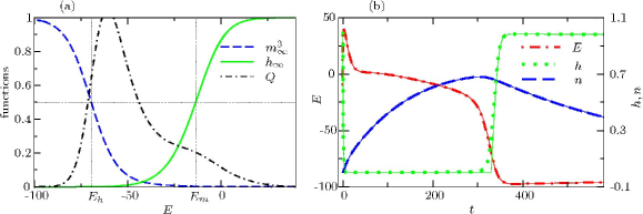
Figure 10: (Color online) (a) The function ${Q}({E})$ defined by (62) in comparisson with ${m^{3}_{\infty}}({E})$ and ${{h}_{\infty}}({E})$. (b) Solutions $({E},{h},{n})$ of the Noble model (4) (thick lines) and of the more accurate version of the Archetypal Model (66) (corresponding thin solid lines).

f:0070

Figure 2(b) shows that the function ${S}({E})$ is relatively small. However, it appears in (15) multiplied by the large factor ${g_{1}}({E})/{f_{h}}({E})$ and thus the values of the product

$${Q}({E})\equiv{g_{1}}({E})\,{S}({E})/{f_{h}}({E}),$$ (62)

are in fact of the order unity over a significant range of voltages as shown in figure 10(a). It is then clear that neglecting this essentially non-zero term in equation (15) leads to the low accuracy of the AM (19). At first glance, this means that in the Noble model (4), during the repolarization phase of the AP, gate ${h}$ is, in fact, not fast compared to other two variables. This would mean that reduction to a two-variable model in that region is not possible. However, as we have discussed in Introduction after the definition of embedding, a replacement of $1$ with a small parameter can, in fact, be a reasonable embedding, and its quality can be assessed by a comparison of the numerical solutions of the original and the embedded problem. Such comparison is provided in figure 3 and shows that the embedding (19) is indeed reasonable although of a not very high accuracy. Thus we suppose that a higher accuracy can be achieved by taking a first-order approximation of the term ${Q}$ in the parameter ${\epsilon}$, rather than zero-order as in the other terms. Let us denote the small parameter associated with the function ${Q}({E})$ by ${\mu}$, ${\mu}>0$. Then the error term after the first-order approximation in ${\mu}$ will be $O({\mu}^{2})$. The error term after the zero-order approximation in ${\epsilon}$ will be, of course $O({\epsilon})$. If we want these two kinds of error terms to be of the same order, we must therefore consider ${\mu}={\epsilon}^{1/2}$. These arguments are formalized by the following improved version of Axiom VII,

• $\underline{{{S}}}({E};{\epsilon})={\epsilon}^{1/2}{\tilde{S}}({E})+O({\epsilon})$, where ${\tilde{S}}({E})\approx{S}({E})$.

Besides, for technical reasons the following, stronger version of Axiom VI will be more convenient for us:

• $\underline{{{m^{3}_{\infty}}}}({E};{\epsilon})\,\underline{{{{h}_{\infty}}}}({E};{\epsilon})={\epsilon}{\tilde{W}}({E})+O({\epsilon}^{2})$, for the same ${\tilde{W}}({E})$ as in Axiom VI.

Substituting Axioms VIa and VIIa into (15), we get

$$\frac{\mathrm{d}{E}}{\mathrm{d}{t}}={g_{1}}{\tilde{W}}({E})-{\epsilon}^{1/2}\frac{{g_{1}}({E})}{{f_{h}}({E})}\,{\tilde{S}}({E})\,\frac{\mathrm{d}{E}}{\mathrm{d}{t}}+O({\epsilon}).$$ (63)

From here we deduce that $\mathrm{d}{E}/\mathrm{d}{t}={g_{1}}{\tilde{W}}+O({\epsilon}^{1/2})$. Substituting this into the right-hand side of (63) we obtain

$$\frac{\mathrm{d}{E}}{\mathrm{d}{t}}={g_{1}}{\tilde{W}}({E})-{\epsilon}^{1/2}\frac{{g_{1}}({E})}{{f_{h}}({E})}\,{\tilde{S}}({E}){g_{1}}{\tilde{W}}+O({\epsilon}).$$ (64)

Thus, after discarding $O({\epsilon})$ and putting ${\epsilon}=1$, we arrive at the following variant of (16),

$$\frac{\mathrm{d}{E}}{\mathrm{d}{t}}=\left({g_{1}}({E})\,{\tilde{W}}({E})+{g_{2}}({E})\,{n}^{4}+{g_{3}}({E})\right)\,\left(1-{\tilde{Q}}({E})\right),$$ (65a)

$${h}={H}({E})\,{\theta}({{E}_{h}}-{E}),$$ (65b)

$$\frac{\mathrm{d}{n}}{\mathrm{d}{t}}={f_{n}}({E})\,\left({{n}_{\infty}}({E})-{n}\right),$$ (65c)

where the first and third equations are satisfied with accuracy $O({\epsilon})$ and the second equation is satisfied only with accuracy $O({\epsilon}^{1/2})$. Here ${\tilde{Q}}({E})={\tilde{S}}({E})\,{g_{1}}({E})/{f_{h}}({E})$ which according to Axiom VIIa should be close to ${Q}({E})$.

We see that in terms of the slow subsystem, the modification simply amounts to multiplying the right-hand side of equation (65a) by a known function of ${E}$. By analogy, it is straightforward to propose an improved version of the AM (19),

$$\begin{split}&\frac{\mathrm{d}{E}}{\mathrm{d}{t}}=\left({g_{1}}({E})\,{M}({E})\,{\theta}({E}-{{E}_{m}})\,{h}+{g_{1}}({E})\,{W}({E})+{g_{2}}({E})\,{n}^{4}+{g_{3}}({E})\right)\,\left(1-{Q}({E})\right),\\ &\frac{\mathrm{d}{h}}{\mathrm{d}{t}}={f_{h}}({E})\,\left({H}({E})\,{\theta}({{E}_{h}}-{E})-{h}\right),\\ &\frac{\mathrm{d}{n}}{\mathrm{d}{t}}={f_{n}}({E})\,\left({{n}_{\infty}}({E})-{n}\right).\end{split}$$ (66)

This improved AM gives solutions very close to those of the Noble system (4), as illustrated in figure 10(b).

Notice that the asymptotic structure of the improved AM (66) is exactly the same as that of (19). Indeed, the difference amounts to redefining the functions ${g_{1}}({E})$, ${g_{2}}({E})$, ${g_{3}}({E})$ via a factor $1-{Q}$, thus the asymptotic theory discussed in section 3.2 is equally applicable to both systems.

Appendix B The high-excitability embedding

For the numerical values of the parameters corresponding to healthy tissue, the voltage upstroke at the beginning of the AP is, in fact, a much faster variable than the ${h}$-gate. Indeed, the voltage speed constant ${g_{Na}}/{C_{M}}=33\frac{1}{3}$ is large compared to the typical values of the ${h}$-gate speed function, $\max\limits_{[{{E}_{m}},{{E}_{Na}}]}{f_{h}}({E})\approx 1$. This speed difference is unaccounted for by Axioms I–VII(a) where these two quantities have the same asymptotic order. However, some features of a typical AP solution depend on the ratio of these quantities in an exponential way.

To take this feature into account, here we construct an improved embedding which takes the ${E}$-vs.-${h}$ speed difference into account. We use an additional embedding with one more artificial small parameter ${\sigma}>0$. Formally, we replace Axiom I with a new Axiom,
Axiom Ia.  $\underline{{{g_{Na}}}}({\epsilon},{\sigma})={\sigma}^{-1}{\epsilon}^{-1}{g_{Na}}.$
This, of course, does not affect the slow-time subsystem (16). The fast-time subsystem (10) now depends on the new parameter ${\sigma}$ and becomes

$$\begin{split}&\frac{\mathrm{d}{E}}{\mathrm{d}{T}}={\sigma}^{-1}{g_{1}}({E})\,{M}({E})\,{\theta}({E}-{{E}_{m}})\,{h},\\ &\frac{\mathrm{d}{h}}{\mathrm{d}{T}}={f_{h}}({E})\,\left({H}({E})\,{\theta}({{E}_{h}}-{E})-{h}\right),\end{split}$$ (67)

where the trivial equation for ${n}$ is omitted as the ${n}$-gate neither changes nor matters on time scales of interest here. The equations (67) appear to be a standard fast-slow Tikhonov system. However, this is deceptive since the specific properties of the right-hand sides lead to a number of nonstandard features. Let us consider the limit ${\sigma}\rightarrow 0$ in this system. In the super-fast time ${s}={T}/{\sigma}$, the ${h}$-gate is a first integral, $\mathrm{d}{{h}}/\mathrm{d}{{s}}=0$, and ${E}$ satisfies the super-fast equation,

$$\frac{\mathrm{d}{E}}{\mathrm{d}{s}}={g_{1}}({E})\,{M}({E})\,{\theta}({E}-{{E}_{m}})\,{h},$$ (68)

depending on ${h}$ as a parameter. The equilibria of this system for which the the right-hand side vanishes, form an unusual set consisting of the lines ${h}=0$ and ${E}={{E}_{Na}}$ and the semi-stripe $\{({E},{h})\}=(-\infty,{{E}_{m}})\times[0,1]$. Hence, the slow set is not a manifold, but consists of pieces of different dimensionalities. This feature is even “more non-Tikhonov” than the many non-standard properties observed in the main embedding. One consequence is that the slow-time subsystem of (67) changes form as the trajectory passes through the various pieces of the slow set. This dependence is substantial: even the dimensionality of the slow system changes. For instance, for a typical AP solution in the beginning of the plateau, the trajectory crosses the ${E}={{E}_{Na}}$ piece, which can be parameterized by ${h}$. Then we have a one-dimensional slow subsystem of (68) (which is in the “fast time” ${T}$) in the form of an equation for ${h}$,

$$\frac{\mathrm{d}{h}}{\mathrm{d}{T}}=-{f_{h}}({{E}_{Na}})\,{h}.$$ (69)

Then, during the later part of the plateau, which proceeds along the one-dimensional piece ${h}=0$, the slow subsystem becomes “zero-dimensional” in the sense that all right-hand sides vanish and all trajectories are fixed points. This corresponds to the fact that the movement along this piece occurs slowly in terms of the parameter ${\epsilon}$, i.e. is infinitely slow not only in terms of time ${s}$ but in terms of time ${T}$ too. Finally, during the repolarization phase of the AP when the voltage ${E}$ drops below ${{E}_{m}}$, the slow subsystem is on the two-dimensional piece but is in fact foliated to one-dimensional pieces, as the right-hand side of the equation for ${E}$ vanishes and the voltage ${E}$ is a first integral,

$$\begin{split}&\frac{\mathrm{d}{E}}{\mathrm{d}{T}}=0,\\ &\frac{\mathrm{d}{h}}{\mathrm{d}{T}}={f_{h}}({E})\,\left({H}({E})\,{\theta}({{E}_{h}}-{E})-{h}\right).\end{split}$$ (70)

Since the equations of this “high-excitability” embedding are at most one-dimensional systems, obviously all of them can be solved in quadratures. This embedding is rather instructive since it demonstrates that a non-Tikhonov embedding might lead to rather untypical consequences. It might also be useful for a number of applications, especially when healthy, well-excitable tissues are concerned. However, the most important applications are those related to the failure of excitation, or of excitation propagation in the case of spatially-extended systems. These processes are observed, however, exactly when the excitability, represented here by formal parameter ${\sigma}^{-1}$, is not so high.

Appendix C Asymptotic synthesis

We assume, for simplicity, that the initial values of the gating variables are given by ${{h}_{0}}=1$, ${{n}_{0}}=0$. Then, depending on the initial trans-membrane voltage ${{E}_{0}}$, there exist three types of solutions of (19) as visualized by the phase portraits in figure 6 and described below:

C.1 Sub-threshold response

If the initial value of ${E}$ is less that the threshold value of the super-slow subsystem (28) i.e. ${{E}_{0}}<{E_{2}}$, the voltage decays towards its global equilibrium ${E_{1}}$:

• The ${h}$-gate relaxes on a time scale $\sim{\epsilon}$ towards its quasi-stationary value ${h}\approx{H}({E})\,{\theta}({{E}_{h}}-{E})$ according to (23). The variables ${E}$ and ${n}$ remain close to their original values of ${E}\approx{{E}_{0}}$, ${n}\approx{{n}_{0}}=0$.

• The voltage decays on a time scale $\sim 1$ towards its equilibrium value ${E_{1}}$ according to (27) (with ${n}=0$). The ${h}$-gate remains close to its quasi-stationary value except, possibly, swiftly moving on a time scale $\sim{\epsilon}$ along its discontinuity as ${E}$ passes through ${{E}_{h}}$. The slow ${n}$-gate remains approximately at ${n}\approx{{n}_{0}}=0$.

C.2 Slow over-threshold response

If the initial value of the voltage is bigger than the threshold value of the super-slow subsystem (28) but smaller than ${{E}_{m}}$ i.e. ${E_{2}}<{{E}_{0}}<{{E}_{m}}$ then the slow subsystem alone is sufficient to describe the AP evolution and the fast Na current is not involved. The voltage makes a relatively small excursion towards the upper systolic branch of the super-slow manifold and approaches it from below:

• The ${h}$-gate relaxes on a time scale $\sim{\epsilon}$ in the same way as in the case of sub-threshold response, except this time the quasi-stationary value of ${h}$ is zero since ${E_{2}}>{{E}_{h}}$.

• The voltage increases on time scale $\sim 1$ towards ${E_{3}}$ i.e. towards the upper part of the systolic branch of the super-slow manifold according to (27) (with ${n}=0$). The slow ${n}$-gate remains approximately unchanged at ${n}\approx{{n}_{0}}=0$.

• The variables ${E}$ and ${n}$ move on a time scale $\sim{\epsilon_{2}}^{-1}$ along the upper systolic branch of the super-slow manifold ${n}={\mathcal{N}}({E})$, according to (28) until they reach the point $({E_{\ast}},{N_{\ast}})$. The ${h}$-gate remains close to its quasi-stationary value of ${h}\approx 0$.

• The voltage ${E}$ jumps on a time scale $\sim 1$ according to (27), towards the diastolic branch of the super-slow manifold. The ${h}$-gate remains close to its quasi-stationary value except, possibly, for a swift movement along the discontinuity of ${H}({E}){\theta}({{E}_{h}}-{E})$ at ${E}={{E}_{h}}$ on a time scale $\sim{\epsilon}$. The slow ${n}$-gate remains approximately at ${n}\approx{N_{\ast}}$.

• The variables ${E}$ and ${n}$ move on a time scale $\sim{\epsilon_{2}}^{-1}$ along the diastolic branch of the super-slow manifold ${n}={\mathcal{N}}({E})$, according to (28). This continues forever, with $({E},{n})$ asymptotically approaching the true equilibrium of the system $({E_{1}},0)$. Gate ${h}$ stays close to its quasi-stationary value ${h}\approx 0$.

C.3 Normal fast-upstroke action potential

If the initial value of the voltage exceeds the threshold of the primary fast-time system (21) i.e. ${{E}_{0}}>{{E}_{m}}$ the fast Na current is activated and a normal fast-upstroke AP, is initiated:

• The variables ${h}$ and ${E}$ change together on a time scale $\sim{\epsilon}$ according to (24) from the point $({E},{h})=({{E}_{0}},1)$ asymptotically (in ${T}\rightarrow\infty$) approaching the point $({E},{h})=\left({{E}_{\infty}}({{E}_{0}},1),0\right)$. The slow ${n}$-gate remains approximately unchanged at ${n}\approx{{n}_{0}}=0$.

• The voltage ${E}$ descends, inasmuch as ${{E}_{\infty}}({{E}_{0}},1)>{E_{3}}$, on a time scale $\sim 1$ towards its higher equilibrium value ${E_{3}}$ according to (27) (with ${n}=0$). Variable ${h}$ remains close to its quasi-stationary value of ${h}\approx 0$. The slow ${n}$-gate remains approximately unchanged at ${n}\approx{{n}_{0}}=0$.

• stages follow which are similar to the corresponding stages in the case of slow over-threshold response.

References

- [1]
- Abramowitz and Stegun [1965] Abramowitz, M. and Stegun, I. A., eds [1965], Handbook of mathematical functions: with formulas, graphs, and mathematical tables, Dover, New York.
- Aliev and Panfilov [1996] Aliev, R. R. and Panfilov, A. V. [1996], ‘A simple two-variable model of cardiac excitation’, Chaos Solitons & Fractals 7, 293–301.
- Attwell et al. [1979] Attwell, D., Cohen, I., Eisner, D., Ohba, M. and Ojeda, C. [1979], ‘The steady state TTX-sensitive (”window”) sodium current in cardiac Purkinje fibres’, Pflugers Arch. 379(2), 137–142.
- Beeler and Reuter [1977] Beeler, G. and Reuter, H. [1977], ‘Reconstruction of the action potential of ventricular myocardial fibres’, J. Physiol. 268, 177–210.
- Bernus et al. [2002] Bernus, O., Wilders, R., Zemlin, C. W., Verschelde, H. and Panfilov, A. V. [2002], ‘A computationally efficient electrophysiological model of human ventricular cells’, Am. J. Physiol. Heart. Circ. Physiol. 282, 2296–2308.
- Biktashev [2003] Biktashev, V. [2003], ‘A simplified model of propagation and dissipation of excitation fronts’, Int. J. of Bifurcation and Chaos 13(12), 3605–3620.
- Biktashev and Biktasheva [2005] Biktashev, V. and Biktasheva, I. [2005], ‘Dissipation of excitation fronts as a mechanism of conduction block in re-entrant waves’, Lect. Notes Comp. Sci. 3504, 283–292.
- Biktashev [2002] Biktashev, V. N. [2002], ‘Dissipation of the excitation wavefronts’, Phys. Rev. Lett. 89(16), 168102.
- Biktashev and Suckley [2004] Biktashev, V. N. and Suckley, R. [2004], ‘Non-Tikhonov asymptotic properties of cardiac excitability’, Phys. Rev. Lett. 93(16), 168103.
- Biktasheva et al. [2003] Biktasheva, I., Biktashev, V., Dawes, W., Holden, A., Saumarez, R. and A.M.Savill [2003], ‘Dissipation of the excitation front as a mechanism of self-terminating arrhythmias’, Int. J. Bif. Chaos 13, 3645–3656.
- Biktasheva et al. [2006] Biktasheva, I. V., Simitev, R. D., Suckley, R. S. and Biktashev, V. N. [2006], ‘Asymptotic properties of mathematical models of excitability’, Phil. Trans. Roy. Soc. Lond. ser. A 364(1842), 1283–1298.
- Cherry and Fenton [2007] Cherry, E. M. and Fenton, F. H. [2007], ‘A tale of two dogs: analyzing two models of canine ventricular electrophysiology’, Am. J. Physiol. Heart. Circ. Physiol. 292, H43–H55.
- Clayton [2001] Clayton, R. H. [2001], ‘Computational models of normal and abnormal action potential propagation in cardiac tissue: linking experimental and clinical cardiology’, Physiol. Meas. 22, R15–R34.
- Courtemanche et al. [1998] Courtemanche, M., Ramirez, R. J. and Nattel, S. [1998], ‘Ionic mechanisms underlying human atrial action potential properties: insights from a mathematical model’, Am. J. Physiol. 275, H301–H321.
- Duckett and Barkley [2000] Duckett, G. and Barkley, D. [2000], ‘Modeling the dynamics of cardiac action potentials’, Phys. Rev. Lett. 85, 884–887.
- Echebarria and Karma [2002] Echebarria, B. and Karma, A. [2002], ‘Instability snd spatiotemporal dynamics of alternans in paced cardiac tissue’, Phys. Rev. Lett. 88(20), 208101.
- Fenton and Karma [1998] Fenton, F. and Karma, A. [1998], ‘Vortex dynamics in three-dimensional continuous myocardium with fiber rotation: Filament instability and fibrillation’, Chaos 8, 20–47.
- FitzHugh [1961] FitzHugh, R. [1961], ‘Impulses and physiological states in theoretical models of nerve membrane’, Biophysical Journal 1, 445–456.
- Glass et al. [1991] Glass, L., Hunter, P. J. and McCulloch, A. D., eds [1991], Theory of Heart Biomechanics, Biophysics, and Nonlinear Dynamics of Cardiac Function, Springer, New York.
- Hinch [2002] Hinch, R. [2002], ‘An analytical study of the physiology and pathology of the propagation of cardiac action potentials’, Progress in Biophysics and Molecular Biology 78, 45–81.
- Hodgkin and Huxley [1952] Hodgkin, A. and Huxley, A. [1952], ‘A quantitative description of membrane current and its application to conduction and excitation in nerve’, J. Physiol. 117, 500–544.
- Holden and Panfilov [1997] Holden, A. V. and Panfilov, A. V., eds [1997], Computational Biology of the Heart, Wiley, New York.
- Iyer et al. [2004] Iyer, V., Mazhari, R. and Winslow, R. L. [2004], ‘A computational model of the human left-ventricular epicardial myocyte’, Biophysical Journal 87, 1507–1525.
- Karma [1993] Karma, A. [1993], ‘Spiral breakup in model equations of action potential propagation in cardiac tissue’, Phys. Rev. Lett. 71, 1103–1106.
- Kohl et al. [2000] Kohl, P., Noble, D., Winslow, R. L. and Hunter, P. J. [2000], ‘Computational modelling of biological systems: tools and visions’, Phil. Trans. R. Soc. Lond. A 358, 579–610.
- Krinsky and Kokoz [1973a] Krinsky, V. I. and Kokoz, Y. M. [1973a], ‘Analysis of equations of excitable membranes — I. Reduction of the Hodgkin-Huxley equations to a second order system’, Biofizika 18, 506–511.
- Krinsky and Kokoz [1973b] Krinsky, V. I. and Kokoz, Y. M. [1973b], ‘Analysis of equations of excitable membranes — III. Membrane of the Purkinje fibre. Reduction of the Noble equations to a second order system. Analysis of automation by the graphs of zero isoclines’, Biofizika 18(6), 1067–1073.
- Luo and Rudy [1991] Luo, C.-H. and Rudy, Y. [1991], ‘A model of the ventricular action potential’, Circ. Res. 68, 1501–1526.
- Mishchenko and Rozov [1980] Mishchenko, E. and Rozov, N. [1980], Differential Equations with Small Parameters and Relaxation Oscillations, Plenum Press, New York.
- Nagumo et al. [1962] Nagumo, J., Arimoto, S. and Yoshizawa, S. [1962], ‘An active pulse transmission line simulating nerve axon’, Proc. IRE 50, 2061–2070.
- Noble [1962] Noble, D. [1962], ‘A modification of the Hodgkin-Huxley equations applicable to Purkinje fibre action and pace-maker potentials’, J. Physiol. 160, 317–352.
- Noble and Rudy [2001] Noble, D. and Rudy, Y. [2001], ‘Models of cardiac ventricular action potentials: iterative interaction between experiment and simulation’, Phyl. Trans. R. Soc Lond. A 359, 1127–1142.
- Rogers [2000] Rogers, J. M. [2000], ‘Modeling the cardiac action potential using B-spline surfaces’, IEEE Trans. of BME 47(6), 784–791.
- Rohr and Kucera [1997] Rohr, S. and Kucera, J. P. [1997], ‘Involvement of the calcium inward current in cardiac impulse propagation: induction of unidirectional conduction block by Nifedipine and reversal by Bay K 8644’, Biophysical Journal 72, 754–766.
- Romashko and Starmer [1995] Romashko, D. N. and Starmer, C. F. [1995], ‘Numerical experiments in a modified Beeler-Reuter cable model — initiating fast (Na) and slow (Ca) waves’, Chaos Solitons & Fractals 5, 417–424.
- Shiferaw et al. [2006] Shiferaw, Y., Qu, Z., Garfinkel, A., Karma, A. and Weiss, J. N. [2006], ‘Nonlinear dynamics of paced cardiac cells’, Ann. N.Y. Acad. Sci 1080, 376–394.
- Simitev and Biktashev [2006] Simitev, R. D. and Biktashev, V. N. [2006], ‘Conditions for propagation and block of excitation in an asympthotic model of atrial tissue’, Biophysical Journal 90, 2258–2269.
- Suckley and Biktashev [2003] Suckley, R. and Biktashev, V. [2003], ‘Comparison of asymptotics of heart and nerve excitability’, Phys. Rev. E 68, 011902.
- ten Tusher et al. [2004] ten Tusher, K., Noble, D., Noble, P. and Panfilov, A. [2004], ‘A model for human ventricular tissue’, Am. J. Physiol. 286, H1573–H1589.
- Tikhonov [1952] Tikhonov, A. N. [1952], ‘Systems of differential equations, containing small parameters at the derivatives’, Mat. Sbornik 31(3), 575–586.
- Tyson and Keener [1988] Tyson, J. J. and Keener, J. P. [1988], ‘Singular perturbation theory of traveling waves in excitable media (a review)’, Physica D 32, 327–361.
- van Capelle and Durrer [1980] van Capelle, F. J. and Durrer, D. [1980], ‘Computer simulation of arrhythmias in a network of coupled excitable elements’, Circ. Res. 47(3), 454–466.
- Weiss et al. [2000] Weiss, J. N., Chen, P.-S., Qu, Z., Karagueuzian, H. S. and Garfinkel, A. [2000], ‘Ventricular fibrillation : How do we stop the waves from breaking?’, Circ. Res. 87, 1103–1107.
- Winslow et al. [2000] Winslow, R. L., Scollan, D. F., Holmes, A., Yung, C. K., Zhang, J. and Jafri, M. S. [2000], ‘Electrophysiological modeling of cardiac ventricular function: from cell to organ’, Annu. Rev. Biomed. Eng. 2, 119–155.
- Zeeman [1972] Zeeman, E. C. [1972], Differential Equations for the Heartbeat and Nerve Impulse, Mathematics Institute, University Of Warwick, Coventry.
- Zipes and Wellens [1998] Zipes, D. P. and Wellens, H. J. J. [1998], ‘Sudden cardiac death’, Circulation 98, 2334–2351.