Systematic Field Theory of the RNA Glass Transition

Abstract

We prove that the Lässig-Wiese (LW) field theory for the freezing transition of the secondary structure of random RNA is renormalizable to all orders in perturbation theory. The proof relies on a formulation of the model in terms of random walks and on the use of the multilocal operator product expansion. Renormalizability allows us to work in the simpler scheme of open polymers, and to obtain the critical exponents at 2-loop order. It also allows to prove some exact exponent identities, conjectured in LW.

Together with DNA and proteins, RNA plays a key role in biology. As such it is important to understand their spatial conformations. While for proteins the lowest-energy fold depends strongly on the chemical constitution, and is only tractable numerically, the problem for RNA is simpler, due to a clear separation in energy scale between primary structure (the sequence), secondary structure (pairing of bases in a fold) and tertiary structure (embedding of a fold in 3-d space). The homopolymer problem (all bases identical) was solved in 1968 by de Gennes deGennes . He finds that the pairing-probability of two RNA-bases with labels $s$ and $t$, counted along the backbone, scales like ${\cal P}(s,t)\sim|s-t|^{-\rho_{0}}$, with $\rho_{0}=3/2$. Real RNA molecules however consist of a sequence of 4 different bases, and their optimal fold depends on this sequence. Experimentally important (see e.g. Tinoco ) is further the observation, that pairings $(s,t)$ and $(s^{\prime},t^{\prime})$ are either nested ($s<s^{\prime}<t^{\prime}<t$) or independent ($s<t<s^{\prime}<t^{\prime}$), which graphically amounts to the rule to draw the sequence and the pairings on the plane without self-intersections (planarity). While the problem of a biological RNA-sequence is best solved numerically, for reference it is crucial to understand the physics of (planar) pairings of a random sequence. This was pioniered by Bundschuh and Hwa (BH) BH . They consider a random pairing model with partition function ($\beta=1/k_{B}T$)

$$Z_{\eta}=\sum_{\Phi}\exp\Big{[}-\beta\sum_{1\leq s<t\leq L}\eta(s,t)\Phi(s,t)\Big{]}\ ,$$ (1)

which is defined as a sum over all planar pairings $\Phi$, such that $\Phi(s,t)=1$ if $(s,t)$ is a Watson-Crick pair, and $0$ otherwise. The pair energy $\eta(s,t)$ is considered as a quenched Gaussian disorder variable $\eta(s,t)$, with

$$\overline{\eta(s,t)}=f,\quad\overline{\eta(s,t)\eta(u,v)}{-}f^{2}=\sigma^{2}\delta{({s{-}u})}\delta{({t{-}v})}.$$

Note that this is an additional approximation from the model of a random sequence seq . A key feature of the above model is that there should be a continuous freezing transition between a weak-disorder phase, at large scales undistinguishable from the homopolymer case, and a strong-disorder glass phase with non-trivial scaling, and of possible biological relevance since the conformation and properties of RNA depends on the sequence disorder, i.e. on the primary structure. This glass phase appears in the BH solution of (1) for the $n=2$ replica case (instead of $n=0$ relevant for the disordered case) and in numerical studies at strong disorder BH ; Krzakala02 . Although the initial BH model is quite simple, this strong disorder phase of random RNA appears to be highly non-trivial and quite difficult to study, making it a challenging problem.

In LW Lässig and Wiese (LW) pioneered a field theoretical (FT) approach for the transition to the glass phase. They showed their model to be renormalizable at first order in perturbation theory and calculated the critical exponents. Using a locking argument (see below), the scaling exponents for random RNA in the strong disorder phase were derived, in good agreement with numerics BH ; Krzakala02 .

It is important to understand if this approach defines a consistent theory to all orders, and if the estimates of LW for the scaling exponents are reliable. We achieve this goal here. Using a formulation of the LW model in terms of interacting random walks (RW) in $d=3$ dimensions, and FT tools developped for polymers and membranes DDG3 ; WieseHabil we show that the LW model is renormalizable to all orders. Our formulation is more convenient for calculations and allows us to derive new scaling relations between exponents, and to calculate critical exponents at second order.

The FT model of LW is defined through perturbation theory in the disorder strength $g=\sigma^{2}$, the replica trick, and the continuum limit where $L\to\infty$. One introduces $n$ replicas of the system, labelled by $\alpha=1,\dots,n$. For the free model (no disorder, i.e. $\sigma=0$) the replicas are not coupled and the expectation value of a product of $N$ contact operators $\Phi_{\alpha}(s_{i},t_{i})$ can be computed exactly. It describes the constrained configuration with $N$ fixed pairings $(s_{i},t_{i})$ $(i=1,\cdots,N)$, i.e. $N+1$ subrings of backbone length $\ell_{0},\cdots,\ell_{N}$ (with $L=\ell_{0}+\cdots+\ell_{N}$). As discussed above, this e.v. is

$${\langle\Phi_{\alpha}(s_{1},t_{1})\cdots\Phi_{\alpha}(s_{N},t_{N})\rangle}_{0}=\ell_{0}^{-\rho_{0}}\ell_{1}^{-\rho_{0}}\cdots\ell_{N}^{-\rho_{0}}$$ (2)

with $\rho_{0}=3/2$ if the $(s,t)$’s form a planar pairing, and $0$ otherwise. The partition function for a single free RNA strand then is $Z_{0}^{(n=1)}={\langle 1\rangle}_{0}={L}^{-\rho_{0}}$.

The average over the disorder $\eta$ generates an attractive interaction between two replicas,

$$\mathcal{H}_{i}=-g_{0}\sum_{\alpha<\beta}\iint_{1\leq s<t\leq L}\Psi_{\alpha\beta}(s,t)$$ (3)

with coupling $g_{0}\propto\sigma^{2}$ and the overlap operator

$$\Psi_{\alpha\beta}(s,t)=\Phi_{\alpha}(s,t)\Phi_{\beta}(s,t)\ .$$ (4)

The quenched disorder average is obtained for $n\to 0$. The averaged free energy $\overline{F}$ for a single strand is

$$\overline{F}=-\overline{\log Z_{\eta}}=\lim_{n\to 0}-{\partial\over\partial n}{Z}_{n}\ ,\qquad{Z}_{n}={\langle\mathrm{e}^{-\mathcal{H}_{i}}\rangle}_{0}\ .$$ (5)

${Z}_{n}$ is the partition function for $n$ interacting replicas. Similarly, the average of an observable $A$, $\overline{A}$, is the $n\to 0$ limit of the average in the interacting theory. These observables are calculated as perturbative series in the disorder strength $g_{0}$. They suffer from short-distance UV divergences. Taking $\rho_{0}$ as an analytic regularization parameter, $\rho_{0}\leq 3/2$, LW show at first order that these UV divergences are poles in $\epsilon=2\rho_{0}-2$ at $\epsilon=0$ and that the theory is 1-loop renormalizable at $\epsilon=0$ ($\rho_{0}=1$). An UV-finite renormalized theory is defined through a renormalization of the disorder strength $g_{0}$ and of the backbone length $L$. This allows to compute at first order the RG $\beta$ function for the disorder strength $g$. It is found to have a UV fixed point $g^{*}\,{>}\,0$ for $\epsilon\,{>}\,0$, in particular for the physical case $\epsilon=1$, $n=0$. $g^{*}$ corresponds to the RNA freezing transition. LW compute also the scaling dimensions $\rho^{\star}$ and $\theta^{\star}$ of the operators $\Phi$ and $\Psi$ at the transition.

Our goal is to construct a FT which reproduces (2). For this we note that $\ell^{-\rho_{0}}$ is the return probability at proper time $\ell$ for a free random walk (RW) in $\mathbb{R}^{d}$ with $d=2\rho_{0}$. Thus we introduce $n$ independent RW’s, $\mathbf{r}_{\alpha},\,\alpha=1,\dots,n$ ($\mathbf{r}_{\alpha}(s)=\{r_{\alpha}^{\mu}(s);\,\mu=1,\dots,d\}$). In order to keep only planar pairings we use $n\times N$ pairs of auxiliary fields $\gamma_{a}^{\alpha}(s)$ and $\tilde{\gamma}_{a}^{\alpha}(s)$ ($a=1,\ldots,N$). The free model is given by the action ($\,\dot{\ }:=\partial/\partial s$)

$$\mathcal{S}_{0}=\sum_{\alpha=1}^{n}\int_{0}^{L}\!{\mathrm{d}}s\,{1\over 4}\Big{[}\dot{\mathbf{r}}_{\alpha}(s)\Big{]}^{2}\,+\,\sum_{\alpha=1}^{n}\sum_{a=1}^{N}\int_{0}^{L}\!{\mathrm{d}}s\,\tilde{\gamma}_{a}^{\alpha}(s)\dot{\gamma}_{a}^{\alpha}(s)$$ (6)

The propagators for $r$ and $\gamma,\tilde{\gamma}$ are

$$\frac{1}{2}\left<\left[r_{\alpha}^{\mu}(s)-r_{\beta}^{\nu}(t)\right]^{2}\right>_{0}=\delta_{\alpha\beta}\delta^{\mu\nu}|s-t|$$ (7)

$${\langle\tilde{\gamma}^{\alpha}_{a}(s)\gamma_{b}^{\beta}(t)\rangle}_{0}=\delta^{\alpha\beta}\delta_{ab}\theta(t-s)\ ,\quad\langle\gamma\gamma\rangle=\langle\tilde{\gamma}\tilde{\gamma}\rangle=0\ ,$$

where $\theta(s)=1$ if $s>0$, and $0$ otherwise.

The key point is that in the large-$N$ limit, the observables for a strand of length $L$ in the LW model correspond to the partition function for a closed RW in our model, with specific boundary conditions (the end points are fixed and there is a creation operator $\tilde{\gamma}$ at the origin and an annihilation operator $\gamma$ at the end). The contact operator $\Phi$ changes to

$$\Phi_{\!\alpha}(s,t){=}{1\over N}\!\sum_{a,b}\!\gamma_{a}^{\alpha}\!(s)\tilde{\gamma}_{b}^{\alpha}\!(s)\delta^{d}[\mathbf{r}_{\alpha}(s){-}\mathbf{r}_{\alpha}(t)]\gamma_{b}^{\alpha}\!(t)\tilde{\gamma}_{a}^{\alpha}\!(t).$$

The pair-contact operator $\Psi_{\alpha\beta}(s,t)$ is still given by (4), and the interaction by (3). The auxiliary fields $\gamma$ and $\tilde{\gamma}$ allow to select planar diagrams by taking $N\to\infty$. For the analysis of the UV-divergences, they are mere spectators. Their importance is that they allow to write an action, and thus to apply established tools to prove renormalizability, and to obtain exponents at higher orders. For the sake of simplicity, we shall not write the $\gamma$’s explicitly in the following. We also note that a $1/N$-expansion is feasible, similar in spirit to OrlandZee2002 for the homopolymer problem.

The model defined by (6) belongs to a class of theories with multilocal interactions, including the Edwards model of polymers and Self Avoiding Manifolds (SAM) DDG3 ; WieseHabil . Its short-distance singularities can be studied by the same Multilocal Operator Product Expansion (MOPE). Indeed, the operator $\Psi$ is a product of bi-local operators $\delta[\mathbf{r}_{\alpha}(s)-\mathbf{r}_{\alpha}(t)]$ and of auxiliary fields $\gamma\tilde{\gamma}$. These auxiliary fields have a very simple propagator and a trivial short-distance expansion, which is a product of $\theta$ functions, multiplying the MOPE of the $\delta$’s. Let us give as examples the configurations which encode the UV singularities relevant at one loop. The short-distance behavior of a single $\Psi$ is given by

$$\Psi_{\alpha\beta}(u,v) \mathop{\simeq}_{v\to u} |u-v|^{-d}\mathbf{1}$$

$$+|u-v|^{1-d}\Big{[}{\dot{\mathbf{r}}_{\alpha}(u)}^{2}\!\!+{\dot{\mathbf{r}}_{\beta}(u)}^{2}\Big{]}+\cdots$$

and is depicted graphically as

$$\parbox{50.58878pt}{\includegraphics[width=50.58878pt]{MOPE-1}}\ \to\ \parbox{50.58878pt}{\includegraphics[width=50.58878pt]{MOPE-2}}$$

Similarly, two $\Psi$’s can coalesce into a single $\Psi$ in three ways. Firstly as

$$\Psi_{\alpha\beta}(u,\!v)\Psi_{\alpha\beta}(u^{\prime},\!v^{\prime})\hskip-13.99995pt\mathop{\simeq}_{u^{\prime}\to u,v^{\prime}\to v}\hskip-13.99995ptC(u^{\prime}\!,\!u;v^{\prime}\!,\!v)\Psi_{\alpha\beta}(u,v)+\cdots$$ (9)

that we depict as

$$\parbox{72.26999pt}{\includegraphics[width=72.26999pt]{MOPE-3}}\ \to\ \parbox{72.26999pt}{\includegraphics[width=72.26999pt]{Psi}}$$

with $C(u^{\prime},u;v^{\prime},v)=\left(|u^{\prime}-u|+|v^{\prime}-v|\right)^{-d}$ the corresponding MOPE coefficient. Secondly as

$$\Psi_{\alpha\beta}(u,\!u^{\prime})\Psi_{\alpha\beta}(v,\!v^{\prime})\hskip-13.99995pt\mathop{\simeq}_{u\to v,u^{\prime}\to v}\hskip-13.99995ptD(u,\!u^{\prime}\!,\!v)\Psi_{\alpha\beta}(v,\!v^{\prime})+\cdots$$ (10)

with $D(u,\!u^{\prime}\!,\!v)\!=\!|u^{\prime}{-}u|^{-d}$ if $u{<}u^{\prime}{<}v$ or $v{<}u{<}u^{\prime}$, and $=0$ otherwise, that we depict as

$$\parbox{72.26999pt}{\includegraphics[width=72.26999pt]{MOPE-4}}+\parbox{72.26999pt}{\includegraphics[width=72.26999pt]{MOPE-7}}\to\parbox{72.26999pt}{\includegraphics[width=72.26999pt]{Psi}}$$

Thirdly as

$$\Psi_{\beta\gamma}(u,\!u^{\prime})\Psi_{\alpha\beta}(v,\!v^{\prime})\hskip-13.99995pt\mathop{\simeq}_{u\to v,u^{\prime}\to v}\hskip-13.99995ptE(u,\!u^{\prime}\!,\!v)\Psi_{\alpha\beta}(v,\!v^{\prime})+\cdots$$ (11)

with $E(u,\!u^{\prime}\!,\!v)\!=\!D(u,\!u^{\prime}\!,\!v)$, that we depict as

$$\parbox{72.26999pt}{\includegraphics[width=72.26999pt]{MOPE-5}}+\parbox{72.26999pt}{\includegraphics[width=72.26999pt]{MOPE-6}}\to\parbox{72.26999pt}{\includegraphics[width=72.26999pt]{Psi-3}}$$

The perturbative expansion involves expectation values of integrals of products of $\Psi$ operators. The short-distance contribution $u{\to}u^{\prime}$ for a single $\Psi(u,u^{\prime})$ in these integrals is given by (Systematic Field Theory of the RNA Glass Transition) and produces an UV divergence. The first term in (Systematic Field Theory of the RNA Glass Transition) gives a UV pole at $d=1$ proportional to the insertion of the unit operator $\mathbf{1}$, while the second one gives a pole at $d=2$ proportional to the operator ${\dot{\mathbf{r}}}^{\,2}$. Similarly, considering now the integrals involving two $\Psi$ operators, the integrals over $u$ and $u^{\prime}$ ($v$ and $v^{\prime}$ fixed) in (9,10,11) give UV poles at $d=2$, proportional to the operator $\Psi$. In both cases, the subdominant terms (represented by the $\cdots$) in the MOPE involve higher dimensional multilocal operators, but do not give any UV pole at $d\leq 2$. Note that although the l.h.s of (11) involves three replicas, the dominant term on the r.h.s. involves only the overlap operator between two replicas. Also note that (10) does not contribute for polymers or SAM’s, since there is a third non-planar diagram, and the sum of all cancel.

This analysis of the UV divergences through the MOPE at first order gives the same results as in LW. It shows that our model is renormalizable to one loop at $d=2$, as expected from the existence of an action, and dimensional analysis.

Our formulation and the MOPE allow to extend this analysis to all orders of perturbation theory DWlong . The dimension $d=2\rho_{0}$ of imbedding space is a dimensional regularization parameter, and short-distance UV divergences appear always as poles in $\epsilon\!=\!d\!-\!2\!=\!2\rho_{0}\!-\!2$. We have shown that the theory is UV finite for $\epsilon<0$ (apart from a trivial “vacuum energy divergence” proportional to the unity operator $\mathbf{1}$). For $\epsilon=0$ the only UV divergences are proportional to the local operator $\dot{\mathbf{r}}_{\alpha}^{\,2}$ and to the bilocal operator $\Psi_{\alpha\beta}$ ($\alpha\neq\beta$). The MOPE also generates multilocal operators involving more than 2 replicas, for instance the 3-replica operator $\Pi_{\alpha\beta\gamma}=\Phi_{\alpha}\Phi_{\beta}\Phi_{\gamma}$. However these operators are not associated to UV divergences, and correspond to irrelevant couplings. The crucial point in this analysis is that, since the interaction in the model involves 2 different replicas $\alpha\neq\beta$, no UV divergence appears which is proportional to the single-replica operator $\Phi_{\alpha}(u,v)$, although $\Phi$ is a “dangerously” marginal operator (it is marginal at $\epsilon\!=\!0$ and relevant as soon as $\epsilon\!>\!0$, like $\Psi$).

The renormalized UV finite theory is defined through the renormalized action $\mathcal{S}_{R}$

$$\mathcal{S}_{R}=\sum_{\alpha}\int_{0}^{L}\!\!{\mathrm{d}}s\,{\mathbb{Z}\over 4}{\dot{\mathbf{r}}_{\alpha}^{\,2}}+g_{R}\mu^{-\epsilon}\mathbb{Z}_{g}\sum_{\alpha<\beta}\iint_{0\leq u<v\leq L}\hskip-30.00005pt\Psi_{\alpha\beta}(u,v)$$ (12)

$\mathbb{Z}$ and $\mathbb{Z}_{g}$ are the wave-function and coupling-constant counterterms, and are series in $g_{R}$ whose coefficients contain the poles in $1/\epsilon$. $\mu$ is the renormalization mass scale. The renormalized field $\mathbf{r}$ and coupling $g_{R}$ are related to the bare ones $\mathbf{r}_{B}$ and $g_{B}$ by $\mathbf{r}_{B}=\mathbb{Z}^{1/2}\mathbf{r}$ and $g_{B}=g_{R}\mathbb{Z}_{g}\mathbb{Z}^{d}\mu^{-\epsilon}$ (this differs from the LW scheme where $s$ is renormalized instead of $\mathbf{r}$ and where $g^{\prime}_{B}=g_{R}\mathbb{Z}_{g}\mathbb{Z}^{2}\mu^{-\epsilon}$). The RG $\beta$ function for the coupling $\beta_{g}$ and the scaling dimension $\chi_{r}$ for the field $\mathbf{r}$ in length-units are

$$\beta_{g}=-\mu\left.{{\mathrm{d}}g_{R}\over{\mathrm{d}}\mu}\right|_{g_{B}}\ ,\quad\chi_{r}={1\over 2}\left(1+\beta_{g}{d\log\mathbb{Z}\over dg}\right).$$ (13)

Since we proved renormalizability, and identified all possible counterterms, we can simplify calculations by using open RWs instead of closed ones, eliminating the $\delta$-function for the closure. Although not all correlation functions are directly interpretable in terms of RNA strands, they are renormalized by the same counterterms, except for one additional boundary term $\mathbb{Z}_{1}$ for each end of the RW, $S_{R}^{\mathrm{open}}=S_{R}^{\mathrm{closed}}+2\mathbb{Z}_{1}$. The (Fourier transformed) partition function $Z^{(1)}$ for a single free open RW then is

$$\parbox{28.90755pt}{\includegraphics[width=28.90755pt]{R1-1-l}}=Z^{(1)}(\vec{q})=\Big{\langle}{\prod_{\alpha=1}^{n}\mathrm{e}^{-\vec{q}(\vec{r}_{\alpha}({\scriptscriptstyle{L}})-\vec{r}({\scriptscriptstyle{0}}))}}\Big{\rangle}=\mathrm{e}^{-n\vec{q}\,^{2}L}\ .$$ (14)

The first-order correction to (14) in the disorder strength is given by the following diagram

$$\parbox{57.81621pt}{\includegraphics[width=57.81621pt]{R1-2-l}}=g_{0}{n(n-1)\over 2}\iint_{0<u<v<L}\hskip-30.00005pt\mathrm{e}^{\vec{q}\,^{2}(2|v-u|-nL)}|v-u|^{-d}.$$ (15)

The last integral is UV divergent when $u\,{\to}\,v$ (bulk) and $u,v\,{\to}\,0$ or $u,v\,{\to}\,L$ (boundary). The corresponding UV pole in $\epsilon=0$ has residue $(1-2L\vec{q}\,^{2})\exp(-n\vec{q}\,^{2}L)$. This partition function for a single open RW is renormalized as

$$Z^{(1)}_{R}(\vec{q},g_{R})=Z_{B}^{(1)}(\mathbb{Z}^{-1/2}\vec{q},g_{B})\,\mathrm{e}^{-2\mathbb{Z}_{1}}\ .$$ (16)

This implies that in the MS scheme the counterterms are at first order $\mathbb{Z}=1+g_{R}(n-1)/\epsilon$, $\mathbb{Z}_{1}=g_{R}(n-1)/4\epsilon$.

To compute $\mathbb{Z}_{g}$ it is simpler to consider the (connected) partition function $Z^{(2)}$ for two distinct interacting open RWs. At first order in $g_{0}$ it is given by

$$\parbox{50.58878pt}{\includegraphics[width=50.58878pt]{R2-1-l}}=Z^{(2)}=g_{0}{n(n-1)\over 2}L^{2}\ .$$ (17)

At order $g_{0}^{2}$ there are 4 UV divergent diagrams, with MOPE given in (9), (10), and (11),

and the corresponding function is renormalized as

$$Z^{(2)}_{R}(g_{R})=\mathbb{Z}^{-d}Z_{B}^{(2)}(g_{B})\mathrm{e}^{-4\mathbb{Z}_{1}}\ .$$ (18)

Care was taken to account for the (missing) zero-mode due to the $\delta$-distribution between the 2 replicas, resulting in the factor of $\mathbb{Z}^{-d}$. To subtract the UV pole at $\epsilon=0$ the counterterm is $\mathbb{Z}_{g}=1+g_{R}(7-4n)/\epsilon$.

This scheme can be continued to 2-loop order DWlong . To simplify the results we subtract minimally $\mathbb{Z}$ and $\mathbb{Z}_{g}\mathbb{Z}^{d}$. Also $\rho(g_{r})$, the dimension of $\Phi$, can be calculated by considering a 2-RW partition function $Z_{\Phi}$ with one $\Phi$ connecting the 2 RW’s. We obtain the RG functions at 2 loops:

$$\beta_{g}(g_{R}) = -\epsilon g_{R}+(5-2n)g_{R}^{2}+(3-2n)(5-2n)g_{R}^{3}$$

$${\chi}_{r}(g_{R}) = {1\over 2}-{n-1\over 2}g_{R}-{(n-1)(4-3n)\over 2}g_{R}^{2}$$ (19)

$$\rho(g_{R}) = 1+{\epsilon\over 2}+(n-1)g_{R}+{(n-1)(3-4n)\over 2}g_{R}^{2}\ .$$

At one loop our results agree with those of LW LW , upon identifying $\beta=\beta_{\scriptscriptstyle{\mathrm{LW}}}$, and $\chi_{r}=1/(2\gamma_{\scriptscriptstyle{\mathrm{LW}}})$. In the physical case of random RNA ($n=0$), our 2-loop results confirm the existence of a UV fixed point (FP) (in our scheme at $g^{*}={1\over 5}\epsilon-{3\over 25}\epsilon^{2}$), describing the freezing transition. The anomalous dimensions of $\Psi$ and $\Phi$ at this FP are

$$\theta^{*} =\Delta_{\psi}(g^{*})=2+\beta_{g}^{\prime}(g^{*})=2-\epsilon-{3\over 5}\epsilon^{2}$$ (20)

$$\rho^{*} =\Delta_{\Phi}(g^{*})=1+{3\over 10}\epsilon+{3\over 50}\epsilon^{2}\ .$$ (21)

On Fig. 1 we plot $\theta^{*}$ (black) and $\rho^{*}$ (grey) from $\epsilon=0$ to $\epsilon=1$ (physical case). The full curves are our 2-loop results, the dashed ones the 1-loop estimates of LW .

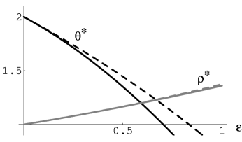
Figure 1: Results for $\theta^{*}$ (black) and $\psi^{*}$ (grey) at 1- (dashed) and 2-loop (solid) order.

The 2-loop corrections do not change much the estimate for $\rho^{*}$, but do change it quantitatively for $\theta^{*}$. This defines another dependent exponent, the roughness $\zeta$ of the height-field $h(r):=\sum_{s<r}\sum_{{t>r}}\Phi(s,t)\sim r^{\zeta}$, as $\zeta=2-\rho$ LW . Since $\Phi_{\alpha}(s,t)\leq 1$, $\left<\Psi_{\alpha\beta}\right>(s,t)\leq\left<\Phi_{\alpha}(s,t)\right>$ and thus $\rho\leq\theta$. This bound is clearly violated by our results for $\epsilon>\epsilon_{\mathrm{c}}\simeq 0.59$. According to LW in this regime the two replicas are locked into a single conformation, $\rho^{*}=\theta^{*}$ and the exponents in the glass phase equal those at the transition

$$\rho_{\mathrm{glass}}=\rho^{*}|_{\epsilon=1}\simeq 1.36,\quad\zeta_{\mathrm{glass}}=2{-}\rho^{*}\simeq 0.64\ .$$ (22)

Finding a small $\epsilon^{2}$ correction to $\rho^{*}$ is important, since it validates the estimates of LW for the exponents of random RNA. Numerical results obtained by Krzakala et al. Krzakala02 in agreement with Bundschuh et al. BH ; Bundschuh.pc give

$$\rho_{\mathrm{glass}}\simeq 1.34\pm 0.003,\quad\zeta_{\mathrm{glass}}\simeq 0.67\pm 0.02$$ (23)

In LW it was also conjectured that the dimensions of $\Phi$ and $\mathbf{r}$ are not independent. Our formalism shows that this is correct and gives an exact relation between $\chi_{r}$ and $\rho$. We remark that the partition function $Z_{\Phi}$ for one $\Phi$ connecting two strands is equivalent to that of two single strands, upon marking a single point on each strand, i.e.

$$Z_{\Phi}=\displaystyle\frac{1}{n^{2}}\Big{[}-\frac{\partial}{\partial{q^{2}}}Z^{(1)}(q)\Big{|}_{q=0}\Big{]}^{2}\ .$$ (24)

At $g^{*}$, together with $\zeta+\rho=2$ LW , this gives

$$\zeta^{*}=2-\rho^{*}=(2-\epsilon)\chi_{r}^{*}\ .$$ (25)

In conclusion, our results for the RNA freezing transition are as follows: First we give a new field theoretical formulation of Lässig-Wiese LW , and prove that their model is renormalizable to all orders in perturbation theory. As a consequence we show that the $\epsilon$-expansion scheme of LW is well defined. Second our formulation allows to simplify the perturbative calculations, in particular by considering open interacting RW’s instead of closed RNA strands. We perform the first 2-loop calculation for the critical exponents $\theta$ and $\rho$, and show that it does not much correct the LW estimate for $\rho$. Third, we derive a new scaling law relating the dimensions of the height field $h$ and $r$. Finally let us mention that we have applied our methods to the denaturation of random RNA under tension, which allows to calculate the extension force curve DHW .

K.W. thanks M. Lässig for the stimulating collaboration which raised many of the questions addressed above.

References

(1)
P.-G. de Gennes, Biopolymers 6, 715 (1968).
(2)
I. Tinoco and C. Bustamante, J. Mol. Biol. 293 (1999) 271.
(3) R. Bundschuh and T. Hwa, Phys. Rev. Lett. 83, 1479
(1999); Europhys. Lett. 59, 903 (2002); Phys. Rev. E 65, 031903
(2002).
(4)
For sequence disorder with different bases, the pair energy
variables are correlated. However, treating them as
independent random variables is numerically an excellent
approximation BH ; Krzakala02 .
(5)
F. Krzakala, M. Mézard, and M. Müller,
Europhys. Lett. 57, 752 (2002).
(6)
M. Lässig and K.J. Wiese, Phys. Rev. Lett. 96 (2006) 228101;
q-bio.BM/0511032, and to be published.
(7)F. David, B. Duplantier and E. Guitter,
Phys. Rev. Lett. 72 (1994) 311; cond-mat/9702136.
(8)
K.J. Wiese,
Polymerized Membranes, a Review,
in Phase Transitions and Critical Phenomena, vol. 19, C. Domb
and J. Lebowitz eds., Academic Press, London (2001).
(9)
H. Orland and A. Zee, Nucl. Phys. B 620,
(2002) 456-76.
(10)
F. David, K.J. Wiese, to be published.
(11)
T. Liu and R. Bundschuh, private communication.
(12)F. David, C. Hagendorf and K. J. Wiese, to be published.