Amplitude-equation approach to spatiotemporal dynamics of cardiac alternans

Abstract

Amplitude equations are derived that describe the spatiotemporal dynamics of cardiac alternans during periodic pacing of one- [B. Echebarria and A. Karma, Phys. Rev. Lett. 88, 208101 (2002)] and two-dimensional homogeneous tissue and one-dimensional anatomical reentry in a ring of homogeneous tissue. These equations provide a simple physical understanding of arrhythmogenic patterns of period-doubling oscillations of action potential duration with a spatially varying phase and amplitude, as well as explicit quantitative predictions that can be compared to ionic model simulations or experiments. The form of the equations is expected to be valid for a large class of ionic models but the coefficients are derived analytically only for a two-variable ionic model and calculated numerically for the original Noble model of Purkinje fiber action potential. In paced tissue, this theory explains the formation of “spatially discordant alternans” by a linear instability mechanism that produces a periodic pattern of out-of-phase domains of alternans. The wavelength of this pattern, equal to twice the spacing between nodes separating out-of-phase domains, is shown to depend on three fundamental lengthscales that are determined by the strength of cell-to-cell coupling and conduction velocity (CV) restitution. Moreover, the patterns of alternans can be either stationary, with fixed nodes, or traveling, with moving nodes and hence quasiperiodic oscillations of action potential duration, depending on the relative strength of the destabilizing effect of CV-restitution and the stabilizing effect of diffusive coupling. For the ring geometry, we recover the results of Courtemanche, Glass and Keener [M. Courtemanche, L. Glass, and J. P. Keener, Phys. Rev. Lett. 70, 2182 (1993)] with two important modifications due to cell-to-cell diffusive coupling. First, this coupling breaks the degeneracy of an infinite-dimensional Hopf bifurcation such that the most unstable mode of alternans corresponds to the longest quantized wavelength of the ring. Second, the Hopf frequency, which determines the velocity of the node along the ring, depends both on the steepness of CV-restitution and the strength of this coupling, with the net result that quasiperiodic behavior can arise with a constant conduction velocity. In both the paced geometries and the ring, the onset of alternans is different in tissue than for a paced isolated cell. The implications of these results for alternans dynamics during two-dimensional reentry are briefly discussed.

I Introduction

Beat-to-beat changes in the T-wave portion of the electrocardiogram (ECG) that reflects the repolarization of the ventricles $-$a phenomenon known as T-wave alternans$-$Lewis , can be a precursor to life-threatening ventricular arrhythmias and sudden cardiac death precur . T-wave alternans have been related to alternations of repolarization at the single cell level Pasetal , thereby establishing a causal link between electrical alternans and the initiation of ventricular fibrillation. Repolarization alternans are characterized by a beat to beat oscillation of the action potential duration (APD) at sufficiently short pacing interval Min . Experiments in both two-dimensional Pasetal and linear strands Foxetal of cardiac tissue, as well as ionic model simulations Foxetal ; Quetal ; Watetal , have shown that the resulting sequence of long and short action potential durations can be either in phase along the tissue (concordant alternans), or can split into extended regions oscillating out of phase (discordant alternans). The latter case is of special importance since it can lead to conduction blocks Foxetal and the initiation of ventricular fibrillation Pasetal . Furthermore, alternans can provide a mechanism of wave breaks that sustain ventricular fibrillation Kar94 ; FeCh02 . The dual role of discordant alternans in the initiation and, potentially, the maintenance of fibrillation provides the motivation to develop a fundamental understanding of this phenomenon.

Experimental FraSim88 and theoretical studies Couetal ; Vin have shown that spatially modulated patterns of alternans associated with quasiperiodic oscillations of APD can arise naturally in a ring of tissue. The terminology of spatially “discordant alternans”, however, originates from the observation of such patterns in periodically paced tissue Pasetal . Their appearance in this context was first attributed to preexisting spatial heterogeneities in the electro-physiological properties of the tissue Pasetal ; Ro01 . Although heterogeneities may certainly be present LaGi96 , and can affect the formation of discordant alternans Quetal , numerical simulations of ionic models in homogeneous tissue Foxetal ; Quetal ; Watetal ; WeKa06 have shown that they are not necessary for their formation. Dynamical properties alone are able to produce the spatially heterogeneous distributions of APD observed in the experiments.

Pioneering studies by Nolasco and Dahlen NolDal and Guevara et al. Gueetal first explained the occurrence of alternans in a paced cell in terms of the restitution relation

$${\rm APD}^{n+1}=f({\rm DI}^{n}),$$ (1)

between the action potential duration at the $n^{th}+1$ stimulus, ${\rm APD}^{n+1}$, and the so-called diastolic interval ${\rm DI}^{n}$. The latter is the time interval between the end of the previous ($n^{th}$) action potential and the time of the $n^{th}+1$ stimulus during which the tissue recovers its resting properties. The restitution relationship describes only approximately the actual beat to beat dynamics because of memory effects that have been modeled phenomenologically through higher dimensional maps ScCa04 ; Fenton ; HaBa99 ; FoBo02 ; ToSc03 . Moreover, recent theoretical studies have highlighted the role of intracellular calcium dynamics in the genesis of alternans ShWa03 ; ShSa05 . In the present paper, we develop the amplitude-equation approach assuming that the simple relationship given by Eq. (1) holds.

If the time interval between two consecutive stimuli is fixed, $\tau={\rm APD}^{n}+{\rm DI}^{n}=const.$ for all $n$, then Eq. (1) yields the map ${\rm APD}^{n}=f(\tau-{\rm APD}^{n-1})$ that has a period doubling instability if the slope $f^{\prime}$ of the restitution curve, defined by ${\rm APD}=f({\rm DI})$, evaluated at its fixed point exceeds unity. As the slope of the restitution curve typically increases when the pacing period is decreased, alternans may develop beyond a critical value of the pacing rate. In extended tissue, the velocity of the activation wavefront also depends on DI, so the oscillations of APD induce oscillations in the local period of stimulation. This, in turn, acts as a control mechanism that tends to create nodes in the spatial distribution of APD oscillations, thus resulting in discordant alternans.

In a previous paper EcKa02a , we sketched the derivation of an amplitude equation that provides a unified framework to understand the initiation, evolution, and, eventually, control of cardiac alternans EcKa02b ; Chretal06 . For one-dimensional paced tissue, the equation takes the form

$$\tau\partial_{t}a=\sigma a-ga^{3}-\frac{1}{\Lambda}\int^{x}_{0}a(x^{\prime})dx^{\prime}-w\partial_{x}a+\xi^{2}\partial^{2}_{x}a,$$ (2)

where $a\simeq({\rm APD}^{n+1}-{\rm APD}^{n})/2$ measures the amplitude of period doubling oscillations in APD, so that nodes separating out-of-phase alternans region correspond to $a=0$, $\tau$ is the pacing period, $\sigma$ and $g$ are coefficients that can be obtained from the map (1), $w$ and $\xi$ are lengthscales that depend on the strength of diffusive coupling between cells, and $\Lambda$ is determined by the dependence of the conduction velocity (CV), denoted by $c$, on diastolic interval. The CV-restitution curve $c({\rm DI})$ is also known as the dispersion curve in the excitable media literature. It should be noted that time can be treated as a continuous variable in this framework because, even though the APD oscillates from beat to beat, the amplitude $a$ of this oscillation defined above varies slowly over many beats close to the period doubling bifurcation. It is this slow spatiotemporal evolution that is described by Eq. (2).

In this paper, we provide a detailed derivation of the amplitude-equation above and extend it to two-dimensional paced tissue. In addition, we extend this approach to treat the important case of one-dimensional reentry in a ring of tissue. For clarity of presentation, we will first derive the amplitude-equation for the ring geometry, and then show how to modify the boundary conditions on this equation to treat paced tissue in one and two dimensions. Although not treated in this paper, the amplitude equation formalism can be extended to higher dimensional maps (that include memory, or the effect of intracellular calcium), provided that the primary bifurcation is period doubling.

The derivation of the amplitude-equation follows the general amplitude equation framework that has been widely used to study the evolution of weakly nonlinear patterns in non-equilibrium systems CroHoh . In the present context of alternans, however, this derivation is made extremely difficult by the stiff nature of ionic models and the fact that the underlying stationary state (with no alternans) corresponds to a train of pulses. To surmount these difficulties, the derivation of the amplitude-equation proceeds in two steps. First, spatially coupled maps, which describe the beat-to-beat dynamics of APD oscillations, including the crucial effect of cell-to-cell coupling, are derived from the underlying ionic models. Second, a weakly nonlinear and multiscale analysis is used to derive amplitude equations from these spatially coupled maps. The weakly nonlinear nature of the expansion is valid close to the onset of the period doubling bifurcation. The multiscale nature of the expansion, which allows us to retain only the two lowest order spatial derivative terms in Eq. (2), is itself justified by the fact that the wavelength of spatial modulation of alternans is large compared to the length scale $\sim\xi$ over which the action potential of a cell is influenced by neighboring cells through diffusive coupling.

The paper is organized as follows. In the next section, we introduce two ionic models and compute their action potential duration and conduction velocity restitution curves. These curves are used to relate quantitatively the ionic models and the amplitude equations. The models considered are the Noble model for Purkinje fibers Nob and a simple two-variable ionic model that captures basic dynamical properties of the cardiac action potential. This model has the advantage that it is simple enough to calculate analytically the restitution curves as well as all the coefficients of the amplitude-equation (2).

Section III is devoted to the derivation of the amplitude equation in the ring geometry. This equation is then used to study the stability of pulses. The results are compared to previous analyses based on coupled maps Couetal ; Vin . Courtemanche et al. Couetal showed that the wavelength of spatial modulation of alternans is quantized in a ring geometry. In the same language that has been used recently to describe discordant alternans in paced tissue, this quantization condition corresponds, in the ring, to the existence of different modes of discordant alternans with an odd number of moving nodes separating out-of-phase regions of period doubling oscillations. The amplitude equation sheds light on the effect of cell-to-cell electrical coupling on the stability of these quantized modes of alternans. In particular, we find that this coupling lifts the degeneracy of an infinite-dimensional Hopf bifurcation so that the mode with one node is the most unstable, in qualitative agreement with the prediction of coupled maps that include a phenomenological description of cell-to-cell coupling Vin . Furthermore, we show that coupling can lead to quasiperiodicity even in the absence of CV-restitution. The effect of diffusive coupling on one-dimensional alternans dynamics in tissue has also been investigated in the context of a stability analysis of FitzHugh-Nagumo type models CytKee02 . This analysis captures the fact that the onset of alternans in tissue can differ from a single cell. However, it does not provide a general framework to make predictions relevant for more realistic ionic models of cardiac excitation or experiments.

We extend our theory to the paced case in section IV. The main result is that discordant alternans results from a pattern-forming linear instability that produces either standing, with fixed nodes, or traveling waves, with moving nodes that separate out-of-phase alternans regions. Whereas in the ring the wavelength of discordant alternans is determined by the ring perimeter, the wavelength in the paced case is independent of tissue size. In the latter, spatial patterns form due to the competing effect of CV-restitution, contained in the nonlocal term in Eq. (2), which tends to create steep spatial gradients of repolarization, and diffusive cell-to-cell coupling contained in the spatial gradient terms, which tends to smooth these gradients. As a result of this competition, the wavelength $\lambda$ of discordant alternans depends on the three fundamental length scales $w$, $\xi$, and $\Lambda$ in Eq. (2), with different scalings $\lambda\sim(w\Lambda)^{1/2}$ and $\lambda\sim(\xi^{2}\Lambda)^{1/3}$ for standing and traveling waves, respectively. We also extend the model to two-dimensional paced tissue. This extension is straightforward under the assumption that the propagation of the front is weakly perturbed by the oscillations in APD. Finally, we discuss briefly nonlinear effects and conduction blocks.

Finally, in sections V and VI we present the discussion and conclusions. Appendix A contains additional details on the derivation of the restitution curves for the two-variable ionic model. Appendix B, in turn, contains the details of the derivation of the integral kernel that couples spatially the iterative maps of the beat-to-beat dynamics. This derivation makes use of the Green’s function for the diffusion equation to obtain an integral expression for the time course of the membrane voltage and hence the APD.

II Ionic models and restitution curves

Our formulation is based on the action potential duration and conduction velocity restitution properties. To obtain the restitution curves, we simulate the ionic models in a one-dimensional strand of paced tissue. We consider the standard cable equation

$$\partial_{t}V=D\,\partial^{2}_{x}V-\left(I_{\rm ion}+I_{ext}\right)/C_{m},$$ (3)

with the membrane current $I_{\rm ion}$, time in units of millisecond (ms), $D=2.5\times 10^{-4}$ cm²/ms, $C_{m}=12\,\mu$F/cm². The external current $I_{ext}$ models a sequence of stimuli applied at $x=0$ at a constant pacing interval $\tau$. We impose zero gradient boundary conditions on $V$ at the two ends of the cable.

In the rest of the paper, we will use two models for the ionic currents. The first is the original 1962 Noble model for Purkinje fibers Nob . The second is a simplified two-variable model with a triangular shaped action potential. This model is more tractable analytically for the purpose of deriving spatially coupled maps of the beat-to-beat dynamics and the length scales $w$ and $\xi$ of the amplitude equation. For higher order ionic models like the Noble model, these coefficients need to be obtained numerically following a procedure detailed in Sec. IV.A. The two-variable model is defined by the total membrane current EcKa02a

$$\frac{I_{ion}}{C_{m}}=\frac{1}{\tau_{0}}\left[S+(1-S)V/V_{c}\right]+\frac{1}{\tau_{a}}h\,S.$$ (4)

This current is the sum of a slow, time-independent, outward current (similar to the potassium current in more realistic ionic models), which repolarizes the cell on a slow time scale $\tau_{0}$, and a fast inward current that is a simplified version of the sodium current. The latter depolarizes the cell in the fast time $\tau_{a}\ll\tau_{0}$. The inactivation of the fast inward current is regulated by the gate variable $h$, which evolves according to

$$\frac{dh}{dt}=\frac{1-S-h}{\tau_{-}(1-S)+S\tau_{+}},$$ (5)

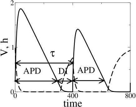
Figure 1: a) Trajectories in the phase plane ($V$, $h$) for the two-variable model [Eqs. (4)-(5)], obtained by simulating $\dot{V}=-I_{ion}/C_{m}$ with an activation interval $\tau=400~{}ms$ and the parameters given in the text. The dashed lines denote the nullclines $h=0$ and $V=0$. b) Time evolution of the voltage $V$ (solid line) and the gate variable $h$ (dashed line) during such trajectory.

where $\tau_{+}$ and $\tau_{-}$ control the time scales of inactivation and recovery from inactivation of this current. In this model the transmembrane voltage $V$ is dimensionless, and $S\equiv[1+\tanh((V-V_{c})/\epsilon)]/2$ is a sigmoidal function. We consider the values of the parameters shown in Table 1. Note that the product of the $h$ and $j$ gates in standard formulations of the sodium current is represented, in the present model, by a single gate $h$. Thus choosing $\tau_{-}$ larger than $\tau_{+}$ produces the same effect of a $j$ gate that controls a slower recovery from inactivation in comparison to inactivation controlled by the $h$ gate. Fig. 1 illustrates the triangular shaped action potentials obtained with this model for stimuli spaced by 400 ms.

$V_{c}=0.1$	$\epsilon=0.005$	$\tau_{0}=150$ ms
$\tau_{a}=6$ ms	$\tau_{-}=60$ ms	$\tau_{+}=12$ ms

Table 1: Parameters used in the simulations of the two-variable model [Eqs. (4)-(5)]

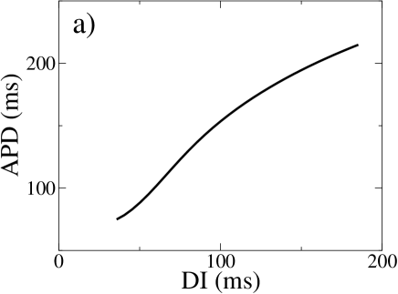
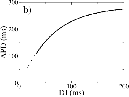
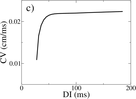
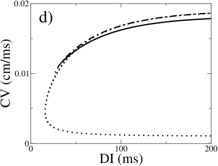
Figure 2: APD- and CV-restitution curves corresponding to the Noble [a) and c)] and two-variable model [b) and d)]. The solid lines correspond to the restitution curves obtained numerically using a S1-S2 protocol. In b) and d) the dotted lines correspond to the theoretical curves given by Eqs. (109) and (104). The dotted-dashed line in d) corresponds to simulations with a finer grid dx=0.001, and dt=0.001, which agree very well with the theoretical predictions, and indicate that, for the usual parameters in the simulations, there is an error of about a 4% in the determination of the maximum conduction velocity.

We have simulated Eq. (3) using the forward Euler method, with a three-point finite difference representation of the one-dimensional Laplacian. We take a mesh size $dx=0.01$ cm, and a time step $dt=0.02$ ms in the case of the two-variable model, and $dx=0.01$ cm, $dt=0.05$ ms, for the Noble model. The thresholds of the transmembrane voltage to define the APD and DI in the two-variable model and the Noble model are $V=V_{c}=0.1$ and $V=-40$ mV, respectively. The restitution and dispersion curves are computed by pacing Eq. (3) in a short cable by an S1-S2 protocol, i.e., the cable is paced at a large period for several beats (sufficient to achieve steady state APD), and then an extrastimulus (S2) is delivered at progressively shorter coupling intervals to vary DI (see Fig. 2). The stimulus is typically applied over ten grid points.

In the limit in which the sigmoidal function $S\equiv(1+\tanh((V-V_{c})/\epsilon))/2$ becomes a step function ($\epsilon\;\rightarrow\;0$), it is possible to calculate both the APD- and CV-restitution curves of the two-variable model analytically (see Appendix A), provided that the ${\rm APD}$ is much larger than the time scale of inactivation of the fast inward sodium current, or ${\rm APD}\gg\tau_{+}$, and that $D/c$ is much smaller than the wavelength of the action potential, or $D/c\ll c{\rm APD}$. Both conditions are satisfied for physiologically relevant conditions. In this limit, the restitution curve is found to be well approximated by the form

$${\rm APD}\simeq\frac{\tau_{+}\tau_{0}}{\tau_{a}}[1-\exp(-{\rm DI}/\tau_{-})]-V_{c}\tau_{0}.$$ (6)

Accordingly, the onset of alternans is given by

$$\frac{{\rm d}\,{\rm APD}}{{\rm d}\,{\rm DI}}\simeq\frac{\tau_{0}\tau_{+}}{\tau_{a}\tau_{-}}\exp(-{\rm DI}/\tau_{-})=1,$$ (7)

or ${\rm DI}_{c}\simeq\tau_{-}\log[(\tau_{0}\tau_{+})/(\tau_{a}\tau_{-})]$, which yields ${\rm DI}_{c}\simeq 96.6$ ms and ${\rm APD}_{c}\simeq 225$ ms for the two-variable model parameters of Table 1.

In the same limit, the CV-restitution curve can be calculated considering a traveling pulse $V(x,t)=V(x-ct)$, and matching the expressions obtained for $V>V_{c}$ and $V<V_{c}$, in the wavefront and the waveback (appendix A). This results in an implicit equation for $c$ (cf. Eq. (104)), that agrees well with the numerical results (see Fig. 2d).

III Ring geometry

The stability of pulses circulating in a ring of tissue was considered previously by Courtemanche et al. Couetal using generic restitution properties of the system as given by Eq. (1). This stability analysis was based on the idea to unravel the ring into an infinite line (then $x\in{\cal R}$, instead of $x\in{\cal R}\;{\rm mod}\;L$). In this manner, the values of a given variable at a previous passage of the pulse through a given point $x$ in the ring, and therefore, at a previous beat, can be identified with the value of that variable at the point $x-L$ (i.e. ${\rm APD}^{n}(x)\equiv{\rm APD}(x+nL)$). This allows to drop the dependence of the different variables on the beat number $n$, and reformulate the maps as delay differential equations. Using this approach, Courtemanche et al. found that, when the slope of the restitution curve is greater than one, the pulses become unstable towards modes of propagation where the values of the APD and conduction velocity vary in space around a mean value. Because of the periodic boundary conditions, the wavelength of these modes is quantized. Without CV-restitution, the ratio of the wavelength to twice the ring perimeter is $1/(2n+1)$ where $n\geq 0$ in an integer. With CV-restitution at onset $c^{\prime}({\rm DI}_{c})\equiv{\rm d}\,c/{\rm d}\,{\rm DI}({\rm DI}_{c})\neq 0$, this ratio becomes irrational and the nodes travel, giving rise to quasiperiodic motion at a given point.

In the analysis of Couetal all the modes were found to bifurcate simultaneously at the same ring perimeter, in an infinitely degenerate Hopf bifurcation. This degeneracy was shown to be broken Vin by the effect of diffusive coupling, which effectively modifies the restitution relation (1) and makes the mode with the longest wavelength (with a single node) bifurcate first. In Vin , the effect of diffusive coupling was considered phenomenologically, assuming a coupling of the APD in neighboring cells given by a simple gaussian kernel. Here, we derive the form of this kernel from an analysis of the two-variable model. The most interesting finding is that this kernel is generally asymmetrical due to the fact that parity ($x\rightarrow-x$) symmetry is broken by the propagation direction of the action potential; it only reduces to a symmetrical gaussian kernel in the limit of infinite conduction velocity. In effect, the way a given cell is influenced by its left and right neighbors is different because these cells are activated at different times by the propagating wavefront. The most interesting consequence of this asymmetry is that it can produce quasiperiodic motion even in the absence of CV-restitution, and modifies the frequency of quasiperiodic oscillations in the presence of CV-restitution.

To study the stability of the pulses we will use an approach slightly different from that in Couetal . We will convert the ring into a linear cable of length $L$ with origin at $x=0$, and index with $n$ the number of times the pulse has traveled around the ring. Accordingly, the variables that characterize the beat-to-beat dynamics depend both on the beat number $n$ and on the space variable $0\leq x\leq L$; the diastolic interval is written as ${\rm DI}^{n}(x)$ and the ring geometry imposes the periodic boundary condition ${\rm DI}^{n}(x-L)={\rm DI}^{n-1}(x)$. Using this parametrization, the ring dynamics is governed by the equations

$$T^{n}(x) = \int_{x-L}^{x}\frac{d\,x^{\prime}}{c[{\rm DI}^{n}(x^{\prime})]}=\int_{x}^{L}\frac{d\,x^{\prime}}{c[{\rm DI}^{n-1}(x^{\prime})]}+\int_{0}^{x}\frac{d\,x^{\prime}}{c[{\rm DI}^{n}(x^{\prime})]},$$ (8)

$${\rm APD}^{n+1}(x) = \int^{\infty}_{-\infty}G(x^{\prime}-x)f[{\rm DI}^{n}(x^{\prime})]\,dx^{\prime},$$ (9)

where $T^{n}(x)$ is the time interval between two consequent activations at the same point. The first equation is just a kinematic equation stating that the period of stimulation at a given point is given by the time it takes a pulse to complete a revolution. The second equation reflects the restitution properties of the system, where we have included an asymmetrical kernel $G(x^{\prime}-x)$ that appears because of the diffusive coupling between neighboring cells. In general, the derivation of the kernel $G(x^{\prime}-x)$ is very difficult and we only derive it explicitly in Appendix B for our two-variable model. The calculation of the kernel involves the inversion of a nonlocal, implicit equation for the APD. Even though we cannot derive this kernel for a general higher order ionic model, this is not a serious limitation. Only the length scales $w$ and $\xi$ in Eq. (2), but not the general form of the amplitude-equation, depend on a precise knowledge of this kernel. Moreover, $w$ and $\xi$ can be calculated numerically for a general higher order ionic model using the procedure detailed in Sec. IV.A.

III.1 Linear stability revisited

Let us thus start reviewing the linear stability analysis of Eqs. (8) and (9). Taking into account that $T^{n}(x)={\rm APD}^{n}(x)+{\rm DI}^{n}(x)$ one can write Eqs. (8), (9) as a single equation for ${\rm DI}^{n+1}(x)$:

$${\rm DI}^{n+1}(x)=\int_{x-L}^{x}\frac{d\,x^{\prime}}{c[{\rm DI}^{n+1}(x^{\prime})]}-\int^{\infty}_{-\infty}G(x^{\prime}-x)f[{\rm DI}^{n}(x^{\prime})]\,dx^{\prime}.$$ (10)

Then, a stationary solution satisfies ${\rm DI}^{*}=\tau-f({\rm DI}^{*})$, where $\tau=L/c({\rm DI}^{*})$ is the period of propagation of the pulse, and we choose the kernel $G(x^{\prime}-x)$ to be normalized, so

$$\int^{\infty}_{-\infty}G(y)dy=1.$$ (11)

We will also assume that the kernel has compact support and that it decays fast enough.

Perturbing around the stationary solution in the form ${\rm DI}^{n}(x)={\rm DI}^{*}+\alpha^{n}e^{ikx}\delta D$, then the stability of the steady state solution is dictated by the value of $\alpha$. If $|\alpha|>1$ an initially small perturbation will grow. Alternans occurs when $\alpha=-1$, and then the resulting instability gives a beat to beat change in the amplitude of APD. Inserting the former expansion in Eq. (10) and linearizing, we obtain that the following equation must be satisfied

$$\alpha=\frac{i\alpha}{2\Lambda k}(1-e^{-ikL})-f^{\prime}\tilde{G}(k),$$ (12)

where we have defined the Fourier transform of the kernel

$$\tilde{G}(k)=\int_{-\infty}^{\infty}G(y)e^{iky}dy.$$ (13)

Here $\Lambda\equiv c^{2}/(2\,c^{\prime})$, defined with $c$ and $c^{\prime}\equiv{\rm d}c/{\rm dDI}$ evaluated at the bifurcation point, is a characteristic length scale associated with CV-restitution.

Furthermore, from the condition ${\rm DI}^{n+1}(x-L)={\rm DI}^{n}(x)$ we obtain the quantization condition $e^{ikL}=\alpha$, so Eq. (12) can be rewritten as

$$\alpha(1-\frac{i}{2\Lambda k})=-f^{\prime}\tilde{G}(k)-\frac{i}{2\Lambda k}.$$ (14)

The onset of the instability is given by $|\alpha|=1$ (implying that the bifurcating mode will have a real wavenumber $k$). This yields

$$f^{\prime 2}|\tilde{G}(k)|^{2}+\frac{f^{\prime}}{\Lambda k}{\cal I}m[\tilde{G}(k)]=1.$$ (15)

The quadratic equation can be solved to obtain the value of $f^{\prime}$:

$$f^{\prime}=\frac{1}{2|\tilde{G}(k)|^{2}}\left(-\frac{{\cal I}m[\tilde{G}(k)]}{\Lambda k}\pm\sqrt{({\cal I}m[\tilde{G}(k)])^{2}/(\Lambda k)^{2}+4|\tilde{G}(k)|^{2}}\right).$$ (16)

The imaginary part of the kernel appears because of asymmetrical coupling. Due to the finite velocity of propagation of the pulses, different points are excited at different times, and the electrotonic coupling of a cell with its left- and right-neighbors will differ. We can assume that this is a small effect, and then:

$$f^{\prime}\simeq\frac{1}{|\tilde{G}(k)|}-\frac{{\cal I}m[\tilde{G}(k)]}{2\Lambda k|\tilde{G}(k)|^{2}},$$ (17)

where we have taken the plus sign in Eq. (16), corresponding to alternans (period doubling). The minus sign would correspond to a steady instability, not studied in this paper.

Since the kernel decays on a spatial scale $\xi$ much shorter than the wavelength of the unstable modes of interest ($\sim L$), the exponential in Eq. (13) can be expanded in the form $e^{iky}\simeq 1+iky-(ky)^{2}/2+\cdots$. It then follows that

$$\tilde{G}(k)\simeq 1-iwk-\xi^{2}k^{2},$$ (18)

where we have defined the coefficients

$$w=-\int_{-\infty}^{\infty}G(y)ydy,\;\;\;\;\xi^{2}=\frac{1}{2}\int_{-\infty}^{\infty}G(y)y^{2}dy.$$ (19)

For an arbitrarily complex ionic model, the form of the kernel $G(y)$ cannot be calculated explicitly, and the coefficients $w$ and $\xi^{2}$ must be obtained from the numerical simulation of the ionic model as described in Sec. IV.A. For the two-variable model with a constant repolarization rate, however, they can be calculated explicitly (Appendix B), giving

$$w = 2D/c,$$ (20)

$$\xi = (D\times{\rm APD}_{c})^{1/2}.$$ (21)

Eq. (21) has the simple physical interpretation that the transmembrane potential $V$ diffuses a length $\sim\xi$ in the time interval of one APD. Therefore, the repolarization of a given cell is influenced by other cells within a length $\sim\xi$ of cable. The imaginary part of $\tilde{G}(k)$ appears because of the asymmetry induced by the propagation of the pulse. This asymmetry vanishes in the limit $c\rightarrow\infty$, where all cells are activated simultaneously, consistent with Eq. (20). For typical values of the parameters in ventricular tissue ($D\sim 10^{-4}-10^{-3}\,\rm{cm}^{2}/\rm{ms}$, $c\sim 10^{-2}-10^{-1}$ cm/ms, ${\rm APD}_{c}\sim 100-200$ ms), the length $\xi$ is of the order of millimeter ($\xi\sim 10^{-1}$ cm), while $w$ an order of magnitude smaller ($w\sim 10^{-2}$ cm). In fact, $w/\xi\sim\xi/(c\times{\rm APD}_{c})$ is the ratio between the diffusive coupling length $\xi$ and the wavelength of the pulse, which is typically an order of magnitude larger.

Introducing expansion (18) into Eq. (17), to lowest order in $k\xi$, we obtain:

$$f^{\prime}=1-\frac{w}{2\Lambda}+\xi^{2}k^{2}.$$ (22)

Intercellular coupling shifts the onset of instability, which occurs for a value of the slope of restitution $f^{\prime}\neq 1$. The slope at onset of alternans will be larger or smaller than one, depending on the relative importance of the different lengthscales of the system. The first mode to bifurcate is the one with largest wavelength, as previously noted by Vinet Vin .

In what follows, in addition to assuming that $wk\ll 1$ and $\xi k\ll 1$, we will also assume that the slope of the CV-restitution curve at the bifurcation point is small so that the length scale $\Lambda$ is much larger that the typical wavelength of alternans modulation, or $\Lambda k\gg 1$. All three conditions turn out to be reasonably well satisfied for the parameters of the Noble model. The last condition $\Lambda k\gg 1$, however, is not fulfilled in the two-variable model because CV-restitution is not weak. In the next section, we will show that it is also possible to treat analytically the case where $\Lambda k$ is of order unity.

Substituting Eq. (22) into Eq. (14), to lowest order we obtain

$$\alpha\simeq-1+iwk-\frac{i}{\Lambda k}.$$ (23)

Both dispersion and asymmetrical coupling result in an imaginary part for $\alpha$, that corresponds to quasiperiodic motion.

If $\alpha=-1$, the instability is strictly period doubling. In this case, the condition $e^{ikL}=\alpha$ implies $k=(2n+1)\pi/L$, with $n=0,1,2,\dots$. To obtain the wavenumber $k$ corresponding to the value of $\alpha$ given in Eq. (23), we assume $k=(2n+1)\pi/L+q$, where $q$ is a small correction $q\ll 1/L$. In this case the condition $e^{ikL}=\alpha$ results into

$$e^{ikL}=(-1)e^{iqL}\simeq(-1)(1+iqL+\cdots)\simeq-1+iw(2n+1)\frac{\pi}{L}-\frac{iL}{\Lambda(2n+1)\pi}+\cdots.$$ (24)

Then, to first order in the correction, the wavenumber is

$$k=(2n+1)\frac{\pi}{L}+\frac{1}{\Lambda(2n+1)\pi}-w(2n+1)\frac{\pi}{L^{2}}.$$ (25)

As $k\sim L^{-1}$, these expressions will be valid if $w,\xi\ll L$, and $\Lambda\gg L$.

The main novel conclusion is that besides the correction to the wavenumber due to CV-restitution derived by Courtemanche et al. Couetal , there is another correction due to asymmetrical coupling. Therefore quasiperiodic motion can occur even with a constant CV. Furthermore, these two effects can balance each other if

$$w=\frac{L^{2}}{\Lambda(2n+1)^{2}\pi^{2}},$$ (26)

in which case the motion becomes strictly periodic even with a finite amount of CV-restitution. In general, these two effects will not exactly balance each other so that the motion will be quasiperiodic with a frequency determined by both the slope of the CV-restitution curve and the asymmetrical coupling strength $\sim w$.

III.2 Derivation of the amplitude equations

Starting from the maps (8) and (9), it is possible to derive equations for the oscillations in period and action potential duration. To that end, we will consider the second iteration of the map (9), and expand it for small values of the amplitude of oscillation. As the change in the value of the APD every two beats is small, the beat number can be treated as a continuous variable. Also, the dispersion relation for the conduction velocity $c=c({\rm DI})$ can be expanded for small oscillations of DI, obtaining from Eq. (8) the corresponding change in the local activation interval, which depends nonlocally on the oscillations of APD. The only non-trivial point in the expansion is the effect of the non-local electrotonic coupling in Eq. (9). Since the kernel decays on a scale $\sim\xi$ shorter than the wavelength of modulation of alternans, it can expanded to obtain a local relation between the change in APD and its local first and second spatial derivatives.

Close to the onset of oscillations we can write

$${\rm APD}^{n}(x) \approx {\rm APD}_{c}\,+\,\delta A\,+\,(-1)^{n}\,a(x,t),$$ (27)

$$T^{n}(x) \approx \tau_{c}\,-\delta\tau\,+\,(-1)^{n}\,b(x,t),$$ (28)

where ${\rm APD}_{c}$ and $\tau_{c}$ are the APD and the period of stimulation evaluated at the bifurcation point of the single-cell map ($f^{\prime}=1$), and we split the perturbations into steady and oscillating parts. Now the basic pacing period will be the traveling time of a pulse around the ring, which in the absence of oscillations is given by $\tau=L/c$, and $\delta\tau\equiv\tau_{c}-\tau\ll\tau_{c}$. Close to the bifurcation point, the steady correction to the APD is, to first order, $\delta A=-\delta\tau/2$. For the oscillating part, since the beat to beat oscillations are taken into account with the terms $(-1)^{n}$, the amplitude of the deviations from the critical values, $a(x,t)$ and $b(x,t)$, vary slowly from beat to beat. We can therefore assume that $a$ and $b$ depend on a continuous time, defined through $n\equiv t/\tau$.

Let us first discuss what are the boundary conditions satisfied by $a(x,t)$ and $b(x,t)$. The transmembrane voltage obeys periodic boundary conditions $V(L)=V(0)$, but, by definition, after a revolution of the pulse along the ring, the system goes into the next beat. Therefore, the values of the period and APD at $x=L$ (that is, right before the end of the revolution) must equal those at $x=0$, at the next beat (i.e. at the beginning of the next revolution). The same is true for the gradients. Then

$$T^{n}(L)=T^{n+1}(0),\;\;\partial_{x}T^{n}(L)=\partial_{x}T^{n+1}(0),$$ (29)

$${\rm APD}^{n}(L)={\rm APD}^{n+1}(0),\;\;\partial_{x}{\rm APD}^{n}(L)=\partial_{x}{\rm APD}^{n+1}(0).$$ (30)

Using Eqs. (27), (28) it is easy to see that, in terms of the oscillations in APD and period, the former boundary conditions become

$$a(L)=-a(0),\;\;\partial_{x}a(L)=-\partial_{x}a(0),$$ (31)

$$b(L)=-b(0),\;\;\partial_{x}b(L)=-\partial_{x}b(0).$$ (32)

These boundary conditions imply that the pattern must have an odd number of nodes. Namely, letting $a(x)\sim e^{ikx}$, one obtains the quantization condition

$$k=(2n+1)\frac{\pi}{L},\;\;n=0,1,2,\dots,$$ (33)

that obtained in Couetal in the limit of zero CV-restitution slope. As we shall see, the corrections to the wavelength come from a phase shift in the slow scale associated with the quasiperiodic motion.

The equation for the oscillations in period is easy to obtain. First, we can write Eq. (8) in differential form

$$\frac{dT^{n}(x)}{dx}=\frac{1}{c[{\rm DI}^{n}(x)]}-\frac{1}{c[{\rm DI}^{n}(x-L)]}=\frac{1}{c[{\rm DI}^{n}(x)]}-\frac{1}{c[{\rm DI}^{n-1}(x)]},$$ (34)

where we take into account that ${\rm DI}^{n}(x-L)={\rm DI}^{n-1}(x)$. Then, substituting expansions (27) and (28) into the former expression, with ${\rm DI}^{n}(x)=T^{n}(x)-{\rm APD}^{n}(x)$, we obtain, at linear order

$$\frac{db}{dx}=\frac{1}{\Lambda}[a(x)-b(x)].$$ (35)

To obtain an expression for $b(x)$ we have to solve Eq. (35), subject to the boundary condition (32). This results into:

$$b(x)=\frac{1}{\Lambda}\int^{x}_{0}e^{(x^{\prime}-x)/\Lambda}a(x^{\prime})dx^{\prime}-\frac{e^{-L/\Lambda}}{\Lambda(1+e^{-L/\Lambda})}\int^{L}_{0}e^{(x^{\prime}-x)/\Lambda}a(x^{\prime})dx^{\prime}.$$ (36)

In order to be able to get an analytical expression for the shift in wavelength, we will take the limit of small dispersion ($L/\Lambda\ll 1$), that will also allow us to compare with the results in Couetal . In this limit, to first order, the exponentials in Eq. (36) can be neglected (equivalent to neglecting the term proportional to $b(x)$ in the right hand side of Eq. (35)). Then, Eq. (36) becomes

$$b(x)=\frac{1}{\Lambda}\int^{x}_{0}a(x^{\prime})dx^{\prime}-\frac{1}{2\Lambda}\int^{L}_{0}a(x^{\prime})dx^{\prime}.$$ (37)

The above equation works well for the Noble model. For the two-variable model, however, it is not strictly valid since $L_{c}/\Lambda>1$. In this case, as we discuss below, the full equation (36) should be used to obtain a good agreement with the simulations of the cable equation (3). For clarity of exposition, we use Eq. (37) in what follows and state the result later for the full equation (36) in the context of a quantitative comparison of the two-variable model and cable equation simulations.

Next, in order to derive an evolution equation for the amplitude $a(x,t)$, we notice that, after two consecutive beats, the APD becomes

$${\rm APD}^{n+2}={\rm APD}_{c}+(-1)^{n+2}a(x,t+2\tau).$$ (38)

Assuming that the APD varies slowly every two beats (which is the case close to the period doubling bifurcation), we can expand $a(x,t+2\tau)\simeq a(x,t)+2\tau\partial a/\partial t$, so

$${\rm APD}^{n+2}={\rm APD}^{n}+(-1)^{n}2\tau\frac{\partial a}{\partial t}.$$ (39)

But, expanding Eq. (9)

$${\rm APD}^{n+1}(x)=\int^{\infty}_{-\infty}G(y)f[{\rm DI}^{n}(y+x)]\,dy\simeq f[{\rm DI}^{n}(x)]-wf^{\prime}\partial_{x}{\rm DI}^{n}(x)+\xi^{2}f^{\prime}\partial^{2}_{x}{\rm DI}^{n}(x),$$ (40)

we can also write ${\rm APD}^{n+2}$ as

$${\rm APD}^{n+2} = f[T^{n+1}-f(T^{n}-{\rm APD}^{n})+wf^{\prime}\partial_{x}{\rm DI}^{n}-\xi^{2}f^{\prime}\partial^{2}_{x}{\rm DI}^{n}]$$ (41)

$$-wf^{\prime}\partial_{x}(T^{n+1}-{\rm APD}^{n+1})+\xi^{2}f^{\prime}\partial^{2}_{x}(T^{n+1}-{\rm APD}^{n+1}),$$

where we have used the definitions in Eq. (19) for $w$ and $\xi^{2}$. Then, using Eqs. (27)-(28), expanding to first order in $w$ and $\xi^{2}$, and taking into account that $f^{\prime}=1$, since we are expanding around the period doubling bifurcation, we have

$${\rm APD}^{n+2} = f[T^{n+1}-f(T^{n}-{\rm APD}^{n})]+w\partial_{x}{\rm DI}^{n}-\xi^{2}\partial^{2}_{x}{\rm DI}^{n}$$ (42)

$$-w\partial_{x}[T^{n+1}-f(T^{n}-{\rm APD}^{n})]+\xi^{2}\partial^{2}_{x}[T^{n+1}-f(T^{n}-{\rm APD}^{n})]$$

$$= f[T^{n+1}-f(T^{n}-{\rm APD}^{n})]+(-1)^{n}\left[-w(2\partial_{x}a-3\partial_{x}b)+\xi^{2}(2\partial^{2}_{x}a-3\partial^{2}_{x}b)\right].$$

In the following we will neglect the term $\partial_{x}b$ compared to $\partial_{x}a$, since from (37) we have that $b\sim a/(\Lambda k)\ll a$, in the limit of small dispersion (i.e. weak CV-restitution). Strictly, the amplitude equation we derive is asymptotically valid close to the bifurcation point if the following scaling relations are satisfied: $a/{\rm APD}_{c}\sim\epsilon^{1/2}$, $b/a\sim 1/(\Lambda k)\sim\epsilon$, $\xi k\sim\epsilon^{1/2}$, and $wk\sim\epsilon$, where $\epsilon\sim\delta\tau/\tau_{c}$ is a dimensionless measure of the distance from the bifurcation point.

Equating now Eqs. (39) and (42), and expanding the second iteration of the map, we obtain the final expression for the evolution of the oscillations of APD, in the limit considered,

$$\tau\partial_{t}a=\sigma a-w\partial_{x}a+\xi^{2}\partial^{2}_{x}a-ga^{3}-b,\\$$ (43)

where $\sigma\equiv f^{\prime\prime}(\tau-\tau_{c})/2$ is of order $\epsilon$, $g\equiv f^{\prime\prime 2}/4-f^{\prime\prime\prime}/6$, and all the derivatives are evaluated at the bifurcation point. These coefficients can be calculated from the curves in Fig. 2. We find the bifurcation in the Noble model to be slightly subcritical, so Eq. (43) must be expanded to fifth order in this case coeffs . For simplicity of exposition, in the following we will focus on the supercritical case. When dispersion is not small, one should keep higher order terms in Eq. (43) involving the oscillation in period $b$. In that case, direct simulation of the original coupled maps (8)-(9) is probably more appropriate, if the goal is to achieve good quantitative agreement with ionic model simulations.

Substituting the expression for $b(x)$ into Eq. (43), we obtain the final amplitude equation in the ring geometry

$$\tau\partial_{t}a=\sigma a-ga^{3}-w\partial_{x}a+\xi^{2}\partial^{2}_{x}a-\frac{1}{\Lambda}\int^{x}_{0}a(x^{\prime})dx^{\prime}+\frac{1}{2\Lambda}\int^{L}_{0}a(x^{\prime})dx^{\prime},$$ (44)

that must be solved with the boundary conditions $a(L)=-a(0)$, $\partial_{x}a(L)=-\partial_{x}a(0)$.

Now, we can consider again the linear stability problem, within our amplitude equation framework. To do that, we write $a(x)\sim e^{ikx+\Omega t}$, with $k$ given by (33), and $\Omega$ complex ($\Omega=\Omega_{r}+i\Omega_{i}$). Separating into real and imaginary parts

$$\tau\Omega_{r}=\sigma-\xi^{2}k^{2}=\sigma-\frac{\xi^{2}}{L^{2}}(2n+1)^{2}\pi^{2},$$ (45)

$$\tau\Omega_{i}=\frac{1}{\Lambda k}-wk=\frac{L}{\Lambda}\frac{1}{(2n+1)\pi}-\frac{w}{L}(2n+1)\pi.$$ (46)

The onset of instability occurs when $\Omega_{r}=0$, which results in $\sigma=\xi^{2}k^{2}$, equivalent to condition (22) when $w/\Lambda\ll 1$. Again, we see that intercellular coupling lifts the degeneracy in the onset of the different modes, since the growth rate depends on the wavenumber of the mode. Clearly, the fastest growing mode is that with the largest wavelength, which corresponds to the mode with a single node. Intercellular coupling also affects the frequency of the quasiperiodic oscillations.

To compare Eqs. (45), (46) with the results from the linear stability of the maps in the previous section, we can factor out the rapid oscillations, so $\alpha^{n}=(-1)^{n}\beta^{n}=(-\beta)^{n}$, and $\beta^{n}=e^{\Omega t}=e^{\tau\Omega n}$, by the definition of the slow time $t=n\tau$. Then, at onset of the instability, $\Omega=i\Omega_{i}$, and

$$\alpha=-\beta=-e^{i\tau\Omega_{i}}\simeq-1+iwk-\frac{i}{\Lambda k},$$ (47)

which is exactly the expression we had obtained before (cf. Eq. (23)).

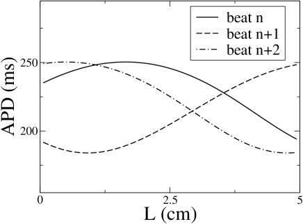
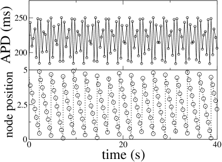
Figure 3: Left panel: distribution of APD at consecutive beats, obtained solving Eq. (3) in a ring of length $L=5$ cm, for the two-variable ionic model. Right panel: evolution in time of the value of the APD at $x=L/2$ (top), and position of the node (bottom), defined as the point $x_{0}$ at which ${\rm APD}(x_{0})=({\rm APD}_{max}+{\rm APD}_{min})/2$.

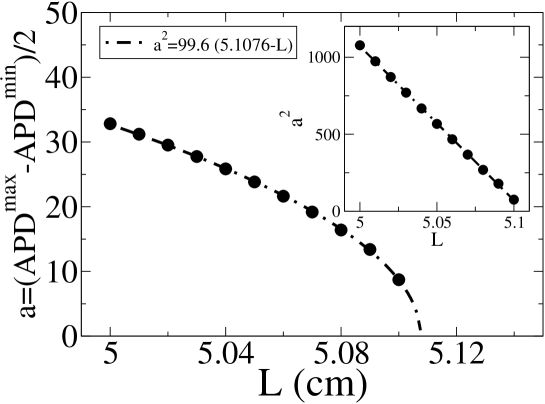
Figure 4: Bifurcation diagram obtained from simulations of the two-variable model in the ring. The bifurcation is supercritical, with a critical ring length of $L_{c}\simeq 5.11$ cm.

We have checked these results with simulations of the two-variable model. As expected, the first mode to bifurcate presents only one node, and the oscillations are quasiperiodic (see Fig. 3). The onset of alternans appears in the simulations for $L_{c}=5.11$ cm, and the phase speed of the bifurcating mode is $v=-\Omega_{i}/k=-1.81\cdot 10^{-3}$ cm/ms, which can be computed from the position of the node as a function of time (see Fig. 3). Using the restitution curves, one obtains that $f^{\prime}=1$ when $\tau_{c}=321.5$ ms, for a conduction velocity of $c=0.0161$ cm/ms. This yields the prediction $L_{c}=5.17$ cm. This prediction, however, neglects the stabilizing effect of the diffusive coupling. Setting $k=\pi/L$, and using (45) with the parameters of the two-variable model, the predicted critical ring length that includes this effect is $L_{c}=5.13$ cm, which is in good agreement with the value $L_{c}=5.11$ cm in the numerical simulations (Fig. 4). Then, setting $L=L_{c}$, the critical wavenumber is $k_{c}=\pi/L_{c}=0.608\;\rm{cm}^{-1}$, and Eq. (46) gives $\Omega_{i}=1.38\cdot 10^{-3}\;\rm{ms}^{-1}$ at the onset of instability, which results in a velocity of the nodes (equal to the phase velocity) $v=-\Omega_{i}/k=-2.27\cdot 10^{-3}$ cm/ms. The discrepancy with the simulation value is due to $1/(\Lambda k_{c})$ corrections. Starting from the full equation (35), which does not assume $\Lambda k_{c}\gg 1$, it is possible to obtain the modified expression for the frequency

$$\tau\Omega_{i}=\frac{\Lambda k}{1+(\Lambda k)^{2}}-wk.$$ (48)

This expression gives $v=-1.85\cdot 10^{-3}$ cm/ms, in almost perfect agreement with the numerical results.

Close to onset, the bifurcating solution is therefore generally in the form of a traveling wave

$$a(x)=\frac{1}{2}(Be^{i(kx+\Omega_{i}t)}+c.c.),\;\;\;k=\pi/L.$$ (49)

Substitution this form in the full nonlinear amplitude equation for the ring (44) and balancing separately real and imaginary parts, we obtain at once that the bifurcation is supercritical with a traveling wave amplitude

$$|B|=\sqrt{\frac{4}{3}\frac{(\sigma-\pi^{2}\xi^{2}/L^{2})}{g}}.$$ (50)

Given the expected universal validity of the amplitude equation (in the limit of small dispersion $\Lambda\rightarrow\infty$), this result implies that the bifurcation to alternans in the ring will always be supercritical if the quasi zero-dimensional bifurcation to alternans in a periodically stimulated small tissue patch is supercritical, which occurs when $g>0$ as in the two-variable model. (Note that it is important to distinguish a small tissue patch from an isolated cell that has a different restitution curve due to the absence of diffusive coupling.) We have checked numerically that the bifurcation is supercritical in the two-variable model (Fig. 4). The amplitude predicted by Eq. (50), however, is about 60% higher than the numerically computed amplitude shown in Fig. 4. This discrepancy can be attributed to $1/(\Lambda k_{c})$ corrections that are not small in the two-variable model due to steep CV-restitution. It should be possible to improve the agreement by including these corrections in the weakly nonlinear analysis. Conversely, if $g<0$, the bifurcation in the ring is subcritical and the saturation amplitude is generally determined by higher order nonlinear terms in the amplitude equation, which can be computed analytically if the bifurcation is only weakly subcritical as in the case of the Noble model coeffs .

IV Paced tissue

The main difference between the ring and the paced case comes from the role of the boundary conditions. While in the ring the periodic boundary conditions result in a quantization condition for the unstable modes, such a condition is absent in the paced case. Thus, the selected wavelength in this latter case must be related to some intrinsic length scale of the system. We show in Fig. 5 simulations of both the Noble and two-variable models. We have done simulations in long cables to highlight the striking spatial regularity of out-of-phase domains of alternans. These patterns suggest that the formation of discordant alternans is caused by a finite-wavenumber linear instability of the basic underlying state, similar to those encountered in other physico-chemical systems, such as Rayleigh-Bénard convection, Taylor-Couette flow, etc CroHoh . The APD oscillations obtained with the Noble model resemble a standing wave (Fig. 5c), and those for the two-variable model a traveling one (Fig. 5d). Thus, at a given point in the tissue, the oscillations in APD are periodic in the first case, and quasiperiodic in the second. We will see how, within the formalism of the amplitude equations, these length scales appear naturally.

To derive the amplitude equations for paced tissue, we must write the equivalent of Eqs. (8)-(9) for this case. Now, the period at a given point will be given by:

$$T^{n}(x)=\tau+\int_{0}^{x}\frac{dx^{\prime}}{c[{\rm DI}^{n}(x^{\prime})]}-\int_{0}^{x}\frac{dx^{\prime}}{c[{\rm DI}^{n-1}(x^{\prime})]},$$ (51)

where $\tau\equiv T^{n}(0)$ is the period of stimulation at the pacing point. This simply means that the period of stimulation at a given point in the tissue is equal to the period of stimulation at the pacing point plus the difference in arrival time between two consecutive pulses. Notice, however, that in differential form this equation is the same as in the ring (cf. Eq. (34)). To complete the system, we can use again Eq. (9), but with a note of care. In fact, in the derivation in the ring, we use translational symmetry to expand the kernel. In the paced case this symmetry is broken and one should, in principle, calculate the kernel for the finite system. When the decay rate of the kernel is fast this does not seem to be necessary. Eqs. (51)-(9), supplemented with non-flux boundary conditions for the oscillations of APD, give a remarkably good agreement with simulations of the ionic models, for all the lengths of tissue considered in this paper. It is interesting to notice that the APD itself does not satisfy these boundary conditions, as rapid spatial variations in APD (“blips”) appear at the two ends of the cable due to the non-flux boundary conditions for $V$. The amplitude $a$ of alternans obtained by taking the difference of APD between two consecutive beats, however, does satisfy very well the non-flux boundary conditions. This can be checked from numerical simulations of the ionic models (see Ref. EcKa02b ).

It follows that the amplitude equations in the bulk remain the same [cf. Eq. (43)], and we only have to modify the boundary conditions. The condition that the period must be equal to the pacing interval at $x=0$, $T^{n}(0)=\tau$, translates into $b(0)=0$. Then, Eq. (35) can be solved for $b(x)$ to give

$$b(x)=\frac{1}{\Lambda}\int_{0}^{x}e^{(x^{\prime}-x)/\Lambda}a(x^{\prime})dx^{\prime}.$$ (52)

As in the previous section, we will assume that the CV-restitution curve is shallow at the bifurcation point, so $\Lambda$ is much larger than the wavelength of the pattern ($\Lambda\gg 2\pi/k$). If this is the case then the exponential in (52) can be neglected and the former relation becomes

$$b(x)\simeq\frac{1}{\Lambda}\int_{0}^{x}a(x^{\prime})dx^{\prime}.$$ (53)

Introducing this into Eq. (43), we arrive at the final expression

$$\tau\partial_{t}a=\sigma a-ga^{3}-\frac{1}{\Lambda}\int_{0}^{x}adx^{\prime}-w\,\partial_{x}a+\xi^{2}\partial^{2}_{x}a.$$ (54)

With the help of equation (54) the formation of the nodes is easy to explain. Let us first neglect the influence of the electrical coupling between cells on the APD (that later on will be shown to be crucial), and consider the equation

$$\tau\partial_{t}a=\sigma a-ga^{3}-b.$$ (55)

Starting at $x=0$ with a constant amplitude of oscillation for the APD $a_{0}$, the oscillation in the period $b$ will increase along the tissue [cf. Eq. (53)], effectively decreasing the value of $a$, until it crosses zero and goes into the branch with opposite phase (see Fig. 6). Thus, the system tends to create discordant alternans spontaneously, through CV-restitution. However, without the derivative terms the gradients become ever steeper, tending to a discontinuous limit as $t\rightarrow\infty$. To see this, we can differentiate Eq. (55), to obtain the steady state equation for the slope of the oscillations in APD $\partial_{x}a=a/\Lambda(\sigma-3ga^{2})$, that can be integrated to obtain $x=\Lambda[\sigma\ln(a/a_{0})-3g(a^{2}-a^{2}_{0})/2]$, with $a_{0}=a(0)=\sqrt{\sigma/g}$. When $a^{2}(x_{0})=\sigma/3g$ the slope becomes infinite, denoting the formation of a singularity at $x_{0}$. The singular behavior originates from the use of the local APD-restitution relation [Eq. (1)] that allows two nearby cells to have different APDs, whereas this is prevented in the cable equation by the spatial diffusive coupling. The distance between singularities can be obtained integrating Eq. (55) from $a^{2}=4\sigma/3g$ (the value after the singularity) to $a^{2}=\sigma/3g$ (the value at the next singularity). Then, we obtain the wavelength (as twice the distance between singularities): $\lambda=2\Lambda\sigma[3/2-\ln(2)]$, that does not correspond to the right length scale for this problem (compare Figs. 6 and 5). Once the derivative terms are included, the agreement between the ionic models and the amplitude-equations becomes very good. To check this point, we have derived the coefficients $w$ and $\xi^{2}$ from the restitution curves of the Noble model (in the two-variable model their values are given by Eqs. (20) and (21)).

IV.1 Measurement of the coefficients $w$ and $\xi$ in the amplitude equation.

To measure the coefficients $w$ and $\xi$ we will consider a case where tissue is paced at a constant period, for values close to, but beyond, the onset of alternans. If we plot the map ${\rm APD}^{n+1}$ in terms of ${\rm DI}^{n}$ corresponding to those simulations (Fig. 7) we obtain a restitution curve that differs from the one obtained using a S1-S2 protocol, where DI is spatially uniform. During discordant alternans the electrotonic currents generated by the spatial modulation of DI along the cable modify the cable restitution curve computed in Appendix A for a spatially uniform DI, which is equivalent to the one obtained using a S1-S2 protocol, $f_{S1S2}$ (see Fig. 2). The cable restitution curve with a spatially modulated DI, which we define as $f_{mod}$, can be different on even and odd beats during discordant alternans because the sign of the spatial gradient of DI in the nodal region alternates from beat to beat. If the system presents no memory, then the difference between $f_{mod}$ and $f_{S1S2}$ is due to the presence of gradients of DI. Expanding the kernel in Eq. (9), we can write:

$${\rm APD}^{n+1}(x)=f_{S1S2}[{\rm DI}^{n}(x)]-w\partial_{x}{\rm DI}^{n}(x)+\xi^{2}\partial^{2}_{x}{\rm DI}^{n}(x)\equiv f_{mod}[{\rm DI}^{n}(x)].$$ (56)

Let us now consider a point in space $x^{*}$ where there is a node in DI, so ${\rm DI}^{n+1}(x^{*})={\rm DI}^{n}(x^{*})={\rm DI}^{*}$. Then, the S1-S2 restitution curve gives the same value at two consecutive beats, so the split in the restitution curve in Fig. 7 will be due to the gradients. Given that the alternans profile in Fig. 7 is, to a good approximation, sinusoidal, then at that point it is also satisfied that $\partial^{2}_{x}{\rm DI}^{n}(x^{*})\simeq\partial^{2}_{x}{\rm DI}^{n+1}(x^{*})\simeq 0$. Subtracting the APD at consecutive beats we have:

$$\Delta{\rm APD}_{1}\equiv f_{mod}[{\rm DI}^{n+1}(x^{*})]-f_{mod}[{\rm DI}^{n}(x^{*})]=w[\partial_{x}{\rm DI}^{n}(x^{*})-\partial_{x}{\rm DI}^{n+1}(x^{*})].$$ (57)

Then, we have

$$w\simeq\frac{\Delta{\rm APD}_{1}}{\partial_{x}{\rm DI}^{n}(x^{*})-\partial_{x}{\rm DI}^{n+1}(x^{*})}.$$ (58)

To calculate the coefficient $\xi$, we just consider the point of tissue $x^{max}$ where $f_{mod}$ has a local maximum, corresponding to an antinode of alternans. At that point $\partial_{x}{\rm DI}^{n}(x^{max})=0$, and then:

$$f_{mod}[{\rm DI}^{n}(x^{max})]=f_{S1S2}[{\rm DI}^{n}(x^{max})]+\xi^{2}\partial^{2}_{x}{\rm DI}^{n}(x^{max}).$$ (59)

In this case $\xi$ can be obtained from the difference between the S1S2 restitution curve and the one obtained during discordant alternans. Defining $\Delta{\rm APD}_{2}\equiv f_{mod}[{\rm DI}^{n}(x^{max})]-f_{S1S2}[{\rm DI}^{n}(x^{max})]$, we have:

$$\xi^{2}\simeq\frac{\Delta{\rm APD}_{2}}{\partial^{2}_{x}{\rm DI}^{n}(x^{max})}.$$ (60)

In Table 2 we show the values of the coefficients calculated in this manner. The comparison between simulations of the amplitude equation (54) using these coefficients and the Noble equations is very good, as shown in Fig. 8.

Model	$\Lambda$	$w$	$\xi$	$\lambda_{theor}/4$	$\lambda_{sim}/4$	$L_{min}$
Noble	49.1	0.045	0.18	2.33	2.6	2.75
Two-variable	3.55	0.031	0.235	1.33	1.1	1.15

Table 2: Values of the parameters in the amplitude equation (2) associated with different length scales, and comparison of the simulated and theoretical wavelengths for the unstable modes in the paced case (all distances in cm). The coefficients $w$ and $\xi$ are obtained analytically from Eqs. (20)-(21) in the two-variable model, and numerically from the APD-restitution curves as explained in the text, for Noble model. The values of $\Lambda$ are obtained from the CV-restitution curves computed numerically, in both cases. The wavelength $\lambda_{theor}$ is predicted from Eq. (67), for Noble, or Eq. (65), for the two-variable model (see text for details), while $\lambda_{sim}$ is obtained from simulations of Eq. (3) in a long cable. These wavelengths give also a good estimate of the minimal length of tissue at which a node appears.

IV.2 Linear stability analysis

Although nonlinear effects determine the saturated amplitude of alternans, the spacing between nodes of discordant alternans, and the velocity of the nodes in the case of traveling waves, are well predicted by linear stability theory close to the bifurcation.

The genesis of discordant alternans can be understood by computing the linear stability spectrum of the spatially homogeneous state ($a=0$). We have calculated this spectrum numerically for different values of $L$, and compared it with the analytical results obtained in the large $L$ limit. The main result is that the wave pattern can emerge from the amplification of either a unique finite wavelength mode, which yields a stationary pattern, or from a discrete set of complex modes that approach a continuum in the limit of large $L$, and yields a traveling pattern (see Fig. 5). There is indeed experimental evidence for both stationary Pasetal and traveling Foxetal waves.

In the large $L$ limit it is possible to obtain analytical expressions for the wavenumber and onset of the waves, using the dispersion related associated to Eq. (54). Differentiating this equation with respect to $x$ and letting $a(x,t)\sim e^{ikx+\Omega t/\tau}$, with both $\Omega\equiv\Omega_{r}+i\Omega_{i}$ and $k\equiv k_{r}+ik_{i}$ complex, yields at once

$$\Omega=\sigma-\xi^{2}k^{2}-i\left[wk-\frac{1}{\Lambda k}\right].$$ (61)

Except for reflection symmetric systems (i.e. system invariant under the transformation $x\rightarrow-x$), or with periodic boundary conditions that impose $k\in{\cal R}e$, the wavenumber will be complex. An instability occurs if there exists a complex wavenumber $k$ for which $\Omega_{r}>0$. It may happen, however, that the unstable mode has a non-zero group velocity $\partial\Omega/\partial k\neq 0$. Then, the instability will grow in the frame moving with the group velocity, but decay at a fixed position. This is the signature of a convective instability CroHoh where perturbations are transported as they grow, similarly to, for instance, Taylor-Couette vortices developing in an axial flow Babetal . In such a situation, patterns are only transient in a finite system (unless a constant forcing is provided), since they disappear through the boundaries in finite time. A sustained instability develops if the group velocity of the unstable mode is zero $\partial\Omega/\partial k=0$, in which case the instability grows at a fixed location in space. This is known as an absolute instability (Fig. 9). The condition

$$\frac{d\Omega}{dk}=0=-2\xi^{2}k-iw-\frac{i}{\Lambda k^{2}}$$ (62)

yields a prediction for the complex wavenumber corresponding to the onset of absolute instability. In the limit $w\rightarrow 0$, it becomes simply

$$k=\pm\frac{\sqrt{3}}{2(2\xi^{2}\Lambda)^{1/3}}-\frac{i}{2(2\xi^{2}\Lambda)^{1/3}},$$ (63)

and corresponds to modes growing exponentially in space. This mode is evident in Fig. 5d, where the amplitude grows away from the pacing point before saturating due to nonlinear effects. There exists a third solution of Eq. (62) that gives a purely imaginary wavenumber (an exponentially decaying mode without sinusoidal part). It can be checked, however, that this mode belongs to the spectrum associated with the equation resulting from differentiating Eq. (54) with respect to $x$, but not to Eq. (54) itself.

Substituting expression (63) into Eq. (61), we deduce that the threshold of absolute instability occurs when

$$\sigma_{th}=(3/2)(\xi/2\Lambda)^{2/3},$$ (64)

with a pattern of wavelength

$$\lambda=\frac{4\pi}{\sqrt{3}}(2\xi^{2}\Lambda)^{1/3}.$$ (65)

This wavelength agrees well with that observed in simulations of the two-variable model (see Table 2). The frequency is, in this approximation, $\Omega_{i}=(3\sqrt{3}/2)(\xi/2\Lambda)^{2/3}$, resulting in $\Omega_{i}\simeq 0.27$ for the two-variable model, and the pattern travels with phase velocity $v_{ph}=-\Omega_{i}/k_{r}$.

We have confirmed the validity of the former analysis by numerically solving the linear eigenvalue problem associated with (54). To obtain the linear spectrum for a given value of $L$, we have linearized and discretized in space Eq. (54), using a finite difference representation of the derivatives and the trapezoidal rule for the integral. Looking for exponentially growing or decaying solutions $a_{i}(t)\sim a_{i}e^{\Omega t/\tau}$, we obtain a set of $N$ coupled linear algebraic equations

$$\Omega a_{i}=\sigma a_{i}-\frac{w}{2dx}(a_{i+1}-a_{i-1})+\frac{\xi^{2}}{dx^{2}}(a_{i+1}+a_{i-1}-2a_{i})-\frac{dx}{\Lambda}\sum^{i-1}_{j=0}\frac{1}{2}(a_{j}+a_{j+1}),\;\;\;i=1\dots N,$$ (66)

where $L=Ndx$, and we typically use $dx=0.05$ cm. The non-flux boundary conditions now become $a_{0}=a_{2}$, and $a_{N+1}=a_{N-1}$. The resulting eigenvalue problem is then solved for the complex growth rate $\Omega=\Omega_{r}+i\Omega_{i}$, and the corresponding eigenmodes. These will be either real (with $\Omega_{i}=0$), in which case we will talk about stationary modes, or come in complex conjugate pairs, resulting in traveling waves. In order to compare with the analytical predictions, we calculate the wavenumber from the number of nodes $n$ of the eigenmodes (of both their real and imaginary parts), as $k_{r}\simeq\pi n/L$.

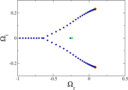
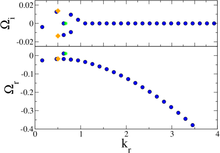
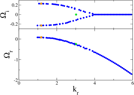
Figure 10: (Color online). Top panels: comparison between the spectra obtained solving the linear eigenvalue problem given by Eq. (66) (circles) and the analytical predictions (diamonds and stars), for the parameters of Noble model (left) at a pacing period of $\tau=258$ ms and $L=20$ cm, and the two-variable model (right), with $\tau=290$ ms and $L=40$ cm. Bottom panels: dependence of growth rate and frequency on the real wavenumber. For the linear eigenvalue problem (circles), the wavenumber has been calculated from the number of nodes $n$ of the eigenmodes $k_{r}\simeq n\pi/L$. The star corresponds to the stationary mode, with $k_{r}=(w\Lambda)^{-1/2}$, $\Omega_{i}=0$, and $\Omega_{r}=\sigma-\xi^{2}/(w\Lambda)$. The diamonds correspond to the results for the standing waves, obtained solving Eq. (62). For the parameters of Noble (left) the first mode to bifurcate is an stationary mode, corresponding to the isolated eigenvalue. For the two-variable model (right), there is a continuous branch of modes that bifurcates first.

From Fig. 10 it can be seen that the spectrum consists of a continuous branch, plus an isolated eigenvalue, whose origin is probably due to the boundary conditions. This can be motivated by noting that $\cos k_{r}x$ is an exact eigenvector of Eq. (54) linearized around $a=0$ that satisfies $\partial_{x}a=0$ at the two cable ends. Substituting that solution into Eq. (54), we obtain $\Omega_{i}=0$, $\Omega_{r}=\sigma-\xi^{2}k^{2}_{r}$, and a wavelength $\lambda=2\pi/k_{r}$ given by

$$\lambda=2\pi(w\Lambda)^{1/2}.$$ (67)

This is in good agreement with the wavelength of standing waves observed in simulations of the cable-Noble equation (Table 2). Although this exact mode only exists for given specific values of the length of the system (when $L$ is an integer multiple of $\lambda/2$), the computed spectrum shows that it also persists for arbitrary values of $L$. The onset of standing waves then is predicted to occur at

$$\sigma_{th}=\xi^{2}/(w\Lambda).$$ (68)

The continuous spectrum ends in the branch points given by the absolute instability, with both $k$ and $\Omega$ complex, corresponding to traveling waves. Then, the bifurcating modes can be either stationary or traveling waves, depending if it is the isolated eigenvalues, or the branch points, that bifurcate first. In the limit $w\rightarrow 0$ the growth rate of the standing wave $\Omega_{r}\rightarrow-\infty$, and the resulting pattern will always be that of traveling waves. There is, therefore, a critical value of $w$ below which the isolated eigenvalue presents a lower growth rate than the branch points, and complex modes that grow exponentially at large $x$ are the most unstable. This is the case for the two-variable model (see Fig. 10), where the modes pass from being convectively to absolutely unstable, as the pacing rate is decreased (Fig. 11). From Eqs. (64) and (68) it can be deduced that traveling waves are favored over stationary waves when $\Lambda=c^{2}/(2c^{\prime})\ll\xi^{4}/w^{3}$, and hence for strong CV-restitution, and vice versa for weak CV-restitution.

Thus, our results demonstrate that the formation of discordant alternans is crucially affected by the effect of electrical coupling (diffusion) on repolarization, in addition to restitution and dispersion. Dispersion is responsible for the formation of nodes and spatial gradients of APD that steepen with time. Diffusion, in turn, tends to spread the APD spatially, and also induces a drift of the pattern away from the pacing site that is induced by the more subtle gradient term ($-w\partial_{x}a$) in the amplitude equation. When dispersion is sufficiently weak, it may be balanced by drift and produce a stationary pattern. In the opposite limit, the tendency for dispersion to form steep gradients of APD is balanced by the spreading effect of diffusion. Nodes then travel, cyclically disappearing (appearing) at the pacing (opposite) end of the cable.

The length scale for the standing waves in the paced case is the same as that for the strictly periodic motion in the ring [see Eq. (26)]. In the former case, however, the non-flux boundary conditions pinned the node (imposed $\Omega_{i}=0$), and that was the only possible wavelength for a bounded state. The only possibility of having a different wavelength, and a traveling node, was to pick up an exponential part ($k$ complex), which is precluded in the ring by the boundary conditions. There, the wavelength is selected by the boundary conditions, and depends on the length of the system. This, in turn, selects the velocity of the node through Eq. (46), that in general will be different from zero. Comparing the critical length scales in both cases, we see that for the mode with largest wavelength in the ring ($n=0$), this results in a critical tissue length of $L_{c}=\lambda/2=5.78$ cm, for Noble, and $L_{c}=\lambda/2=5.17$ cm for the two-variable model. Thus, the length scale in the ring is comparable with the one in the paced case for the Noble model, while for the two-variable model it is significantly larger (see Table 2).

IV.3 Stability diagrams

To compare with previous numerical and experimental results we have calculated the different solutions of the Noble and two-variable models as a function of cable length $L$ and pacing period $\tau$. As can be seen in Fig. 12 these results are in good agreement over a wide range of $L$ and $\tau$ with those obtained simulating the amplitude equations. In particular, discordant alternans appear as soon as the cable is long enough to accommodate roughly a fourth of a wavelength, as given by expressions (67) and (65) (see Table 2). Several comments are in order regarding our results.

(i) The transition from concordant to discordant alternans occurs as the length of the tissue is increased, but the transition line remains nearly constant with increasing pacing rate. This seems to contradict the results obtained in Pasetal , where a transition from concordant to discordant alternans was reported as the pacing rate was increased. In typical models, the slope of CV-restitution is small for large values of DI, but increases very rapidly for small values of DI (see, for instance, the CV-restitution curve of the Noble model in Fig. 2b). Thus, as the pacing rate is increased, the amplitude of alternans grows thereby engaging the steep part of the CV-restitution curve and causing a transition to discordant alternans. This does not occur in the Noble model since there is a reverse period-doubling bifurcation at larger pacing rates by which the steady state regains stability, and the oscillations never get to grow enough, but we have checked this point with simulations of the Beeler-Reuter equations (not shown here). Within our amplitude equations this effect can not be captured since we are expanding around the period-doubling bifurcation point, where the slope of the CV-restitution is fixed. However, it can be observed with the coupled map equations.

(ii) Discordant alternans appear directly from the rest state. This was already observed in simulations of the Beeler-Reuter model Watetal , for lengths of tissue $L\gtrsim 5$ cm. As can be seen in Fig. 5 of that paper, the number of nodes increases with the size of the tissue. This is also the case in our simulations of the Noble model (Fig. 5) where, close to onset, the oscillations of APD adopt a sinusoidal form, with a well defined wavelength. A similar result was observed in Quetal , where the Luo-Rudy model was modified to obtain several APD and CV-restitution curves. In agreement with our results, when the slope of CV-restitution was large at onset, a direct transition to discordant alternans was observed, while, in the case of a shallower curve, the primary transition was to concordant alternans, discordant alternans only appearing when the oscillations in APD grew enough to explore the steep part of the CV-restitution curve.

(iii) The onset of alternans in an extended tissue is delayed with respect to that of the single cell (as given by Eq. (1)). This restabilizing effect is due to a combination of diffusive coupling effects and CV-restitution (see Eqs. (68)-(64)), that induces oscillations in the period of stimulation that effectively act as a control mechanism. In Eq. (54) this effect is produced by the integral term. As is readily seen in Fig. 12 from the diagrams of the Noble and two-variable models, the larger the slope of CV-restitution is at the critical point $f^{\prime}=1$ (the smaller $\Lambda$ is), the larger the value of the restabilization.

(iv) The nodes separating regions oscillating out of phase may be stationary (Noble model), or traveling (two-variable model). Since this distinction occurs already at onset, and there is no transition from one case into the other as the pacing rate is increased, the selected type must depend on the specific ionic model considered. There is experimental evidence for both types of patterns Pasetal ; Foxetal . In real tissue, however, other effects not considered here, such as gradients of restitution properties, could be important, and affect the motion of the node. In the experiments in Foxetal the tissue was paced from both ends, with identical results, which seems to suggest that gradients are not important in that case. In other situations, however, the gradient terms could become important, and create a drift that opposes or reinforces the effect of dispersion.

IV.4 Nonlinear state: conduction blocks and front solutions

Nonlinearities are mainly responsible for saturating the amplitude of the linear modes, although both the wavelength and evolution of the pattern generally vary with distance from onset. Furthermore, at high amplitudes conduction blocks can be produced, which are the main mechanism for the induction of reentry. Recently, systems of coupled maps similar to Eqs. (1) and (8) have been used to study the appearance of conduction blocks FoGi02 ; HeRa05 ; CoVi05 . They are often produced right after the first node in the APD oscillations FoGi02 , thus stressing the importance of discordant alternans for the induction of reentry. Furthermore, the position of the wave block has been shown to vary if the system presents traveling nodes HeRa05 .

Although strictly valid only close to onset, we will use our amplitude equations to get an idea on where conduction blocks can be formed. A conduction block occurs wherever the APD is large enough, so ${\rm DI}=\tau-{\rm APD}<{\rm DI}_{min}$, being ${\rm DI}_{min}$ the minimum diastolic interval necessary for propagation. Let us first neglect the diffusive coupling. Then, using Eq. (55), which is the amplitude equation corresponding to the maps (1) and (8), it is easy to show that the maximum value of the APD occurs just after the discontinuity (see Fig. 6). Considering that the system has reached steady state, and taking the spatial derivative of Eq. (55), we obtain $\partial_{x}b=(\sigma-3ga^{2})\partial_{x}a$. Using that $\partial_{x}b\simeq a/\Lambda$ to eliminate $b$, then, from

$$\partial_{x}a=\frac{a}{\Lambda(\sigma-3ga^{2})}$$ (69)

we obtain that the discontinuity occurs when $a^{2}=\sigma/3g$. At that point $b=\sigma a-ga^{3}=-2\sigma^{3/2}/(3\sqrt{3g})$, if we take the minus sign for $a$. As $b$ is continuous through the discontinuity of APD (Fig. 6), the value of $a$ after the discontinuity can be calculated from

$$ga^{3}-\sigma a+b=0,$$ (70)

which gives $a=2\sqrt{\sigma/3g}$. Then, the conduction block occurs at a value of the period implicitly given by

$${\rm DI}_{min}=\tau-A_{c}-2\sqrt{\sigma/3g},\;\;{\rm with}\;\;\sigma=\frac{1}{2}f^{\prime\prime}(\tau-\tau_{c}),$$ (71)

and at a point in space given by the position of the first singularity, or

$$x_{0}=\frac{1}{2}\Lambda(1-\ln\sqrt{3})f^{\prime\prime}(\tau-\tau_{c}),$$ (72)

obtained solving Eq. (69) with the initial condition $a(0)=\sqrt{\sigma/g}$.

One should be very careful when considering this latter result, since the addition of diffusive effects changes the position of the node, and can make it travel. The reason is that, without diffusion, arbitrarily steep gradients can develop, that prevent the node from moving. Once diffusive effects are included, this is no longer the case, and the node travels, unless its motion is balanced by the drift term. In fact, there is a close analogy between the amplitude equation (54) and the real Ginzburg-Landau equation that has been extensively studied in the context of phase transitions and front propagation CroHoh . The dynamics is richer here because the integral term originating from dispersion causes a non-local interaction of the fronts separating two out-of-phase oscillating regions with the pacing end of the cable.

This is easier to see assuming that both dispersion and the drift terms are small. Then, to first order, one recovers the Ginzburg-Landau equation

$$\tau\partial_{t}a=\sigma a+\xi^{2}\partial^{2}_{x}a-ga^{3},$$ (73)

that has a stationary solution in the form of a front $a_{0}(x)=\sqrt{\sigma/g}\tanh[\sqrt{\sigma/(2\xi^{2})}(x-x_{0})]$, connecting at $x=x_{0}$ regions oscillating out of phase. Then, to calculate the correction due to dispersion and asymmetric coupling, we can set $a(x,t)=a_{0}(x,x_{0}(t))+a_{1}(x,t)$, which, assuming $a_{1}$ small, results to first order in

$$(\sigma+\xi^{2}\partial^{2}_{x}-3ga_{0}^{2})a_{1}=\tau\partial_{t}a_{0}+w\partial_{x}a_{0}+\frac{1}{\Lambda}\int^{x}_{0}a_{0}(x^{\prime})dx^{\prime}.$$ (74)

In order for the system to have a solution, the right hand side must be orthogonal to the left eigenvector of the linear operator, which in this case is simply $\partial_{x}a_{0}$ since the operator is self-adjoint. Then, we obtain

$$-\tau\frac{dx_{0}}{dt}\int^{L}_{0}[\partial_{x}a_{0}(x^{\prime})]^{2}dx^{\prime}+w\int^{L}_{0}[\partial_{x}a_{0}(x^{\prime})]^{2}dx^{\prime}+\frac{1}{\Lambda}\int^{L}_{0}\partial_{x}a_{0}(x^{\prime})\left[\int^{x^{\prime}}_{0}a_{0}(x^{\prime\prime})dx^{\prime\prime}\right]dx^{\prime}=0.$$ (75)

Evaluating the integrals, it is found that the motion of the node is given by

$$\tau\frac{dx_{0}}{dt}=w-\frac{3}{\Lambda}\sqrt{\frac{\xi^{2}}{2\sigma}}x_{0}.$$ (76)

For arbitrary dispersion the expression for the motion becomes more complicated, but the effect is essentially the same. The gradient term corresponding to $w$ makes the node move with constant velocity away from the pacing point, while the integral term provides a ramp that makes one phase of oscillation preferred over the other. When dispersion is weak, there is a point at which the two effects balance each other and the node relaxes to the equilibrium position

$$x_{0}^{eq}=\frac{w\Lambda}{3}\sqrt{\frac{2\sigma}{\xi^{2}}},$$ (77)

which differs markedly from the prediction that neglects diffusive coupling given by Eq. (72).

IV.5 Two-dimensional paced tissue

Let us now generalize our formalism to the case of a square piece of tissue paced at one corner. The equivalent of Eq. (43) is simply

$$\tau\partial_{t}a=\sigma a-ga^{3}-b-w\,(\hat{\bf n}\cdot\nabla)a+\xi^{2}\nabla^{2}a,$$ (78)

where $\hat{\bf n}$ is a unit vector normal to the direction of propagation of the wavefront, and we impose non-flux boundary conditions on the boundaries of the tissue.

Now the determination of the period at a given point would involve the integral along the path traveled by the wavefront. In particular, we obtain the condition for the oscillations in period:

$$(\hat{\bf n}\cdot\nabla)b=\frac{a}{\Lambda}.$$ (79)

In general this is a complicated problem, since we have to know the normal to the wavefront at any given point. A major simplification occurs if we assume that the oscillations in APD do not affect the form of the propagating wavefront, which is the same as to say that the azimuthal variations of APD are small compared with the radial ones. Then, as long as the thickness of the wavefront is small compared with the size of the tissue, it can be assumed that, except for narrow boundary layers at the borders of the tissue, the propagation of the wavefront is perfectly circular. In this case, Eq. (78) can be rewritten as:

$$\tau\partial_{t}a=\sigma a-ga^{3}-\int^{r}_{0}adr^{\prime}-w\,\partial_{r}a+\xi^{2}\nabla^{2}a.$$ (80)

In the far field limit, these equations reduce to Eq. (54), with the node now becoming a circular line. We therefore expect to be a minimum tissue size for the node to form (Fig. 13a), as in the one-dimensional case. This was already observed in experiments Pasetal and numerical simulations of ionic models Watetal , where after a few beats, a nodal line was formed at the corner opposite the pacing point, and then moved towards it. Close to the pacing point, however, the motion of the node becomes nontrivial, because of curvature effects. Besides the term $-w\partial_{r}a$ that tends to make the nodal line move in the radial direction away from the pacing point, there is a contribution to the drift in the direction normal to the interface coming from the Laplacian, this being positive or negative depending on the curvature of the interface. As the nodal line is always perpendicular to the boundaries, its curvature depends on its position on the square. When the tissue is large enough so in the one-dimensional case the node would form in the region with positive curvature (close to the pacing point), this extra effect may be enough to make it travel (Fig. 13).

V Discussion

T-wave alternans is thought to play a key role in the transition from normal heart rhythm to reentrant tachycardia and fibrillation. Alternans has been shown to induce spiral break-up Kar94 ; Co96 , leading to a disordered spatio-temporal state that is usually identified with fibrillation. For this reason, it has been hypothesized that a steep restitution curve may be a possible determinant of the transition from VT to VF Kar94 ; Co96 . Although some experiments support this hypothesis Fib , there is so far no conclusive evidence GiOt97 . From a theoretical point of view, and despite earlier progress Kar94 , we still do not have a complete understanding on how alternans affects the stability of spirals. Numerical simulations show that break-up occurs when the amplitude of alternans oscillation grows enough to induce conduction blocks, which typically happens away from the spiral core. However, there is presently no theory that predicts the spatial distribution of alternans in a spiral wave. Topological arguments impose the existence of a nodal line (also termed line defect) GoKa96 , with a jump in $2\pi$ in the phase of the oscillation, stretching from the core of the spiral to the boundaries. Thus, discordant alternans is always present, but what determines the motion of the nodal line, and whether it is important for spiral break-up is not entirely clear, except far from the spiral core where the dynamics is essentially one-dimensional.

In the present paper, we have considered the simpler cases of one and two-dimensional paced tissue and a circulating pulse in a ring geometry, and derived an equation for the spatio-temporal dynamics of small amplitude alternans in these states. Although conduction blocks fall out of the scope of the present theory, since it only considers small variations in conduction velocity, the results do shed light on where conduction blocks will occur. For that one can look at the distribution of APD and locate the places where it is larger than a critical value. To study the evolution after a conduction block has occurred, one has to resort again to simulations of the original equations.

A circulating pulse in a ring has long been considered as a simplified model of anatomical reentry Mi14 . For rings smaller than a critical value, oscillations in APD appear FraSim88 . An understanding of these oscillations can be helpful in terminating anatomical reentry circuits. In this case discordant alternans is always present, and its wavelength is determined by the length of the ring, with the fastest growing mode having $\lambda\simeq 2L$.

In the paced case, it has been shown Pasetal that the gradients of repolarization created during discordant alternans offer a substrate for conduction block, leading to reentry and ventricular fibrillation. We have shown here that discordant wave patterns Pasetal ; Foxetal ; Quetal ; Watetal result from a finite wavelength linear instability. Hence, their formation requires a minimum tissue size $L_{min}\sim\lambda/4$, required for at least one node to form. The value of $L_{min}$ that we measure in simulations of reaction-diffusion models are actually close to $\lambda/4$ with $\lambda$ predicted by Eq. (67) and Eq. (65), respectively (Table 2). This lengthscale is similar in two-dimensional paced tissue, although in this case, curvature of the nodal line may affect the motion of this line. In both paced one- and two-dimensional tissue and the ring geometry, the onset of alternans in tissue is different than in a paced isolated cell because alternans, in tissue, is manifested as a wave and diffusive coupling tends to smooth out spatial gradients of APD.

The paced and reentrant geometries studied in the present paper also form the basis to develop a theory of the dynamics of alternans in the presence of spiral waves, which has been the subject of both experimental and numerical studies GoKa96 . Far from the core, the spiral is similar to the two-dimensional paced case. In the case where nodes move towards the pacing site in a one-dimensional cable, the nodal line should form a spiral with an opposite chirality as the propagating spiral wave front. This opposite chirality is imposed by the fact that the nodal line moves inward towards the core under the effect of a sufficiently steep, positively sloped, CV-restitution curve, and under the assumption that cellular alternans is driven by APD restitution. The wavelength of the nodal line spiral far from the spiral core should be equal to the wavelength of discordant alternans in the one-dimensional paced case. This should match to the nodal line expected from one-dimensional reentry close to the spiral core. Then, the nodal line should extend straight out of the spiral core in the simplest limit of a constant wave speed where the wavelength of discordant alternans diverges far from the core. A theory for the spiral must, therefore, reduce to the two cases studied in this paper in the appropriate limits. The development of a theory of alternans in this case remains a fascinating task for future work.

VI Conclusions

We have derived an equation that describes the spatio-temporal dynamics of small oscillation alternans in cardiac tissue. Our formulation is based on the restitution properties of the system, and takes also into account intercellular coupling, which is crucial in order to derive the correct threshold pacing rate and lengthscale of discordant alternans. For a simplified two-variable ionic model, we have been able to calculate these coefficients, and show that our reduced description agrees well with numerical simulations of the model. We have also considered the more realistic Noble model, and measured these coefficients numerically, stressing the generality of our formulation. We have applied our formulation to two different cases, a paced tissue and a circulating pulse in a ring.

In the ring, the amplitude equation predicts that both dispersion and intercellular coupling affect the frequency of the motion, and the oscillations of APD are typically quasiperiodic. There is a particular value of the length of the ring where these two effects balance each other, and the oscillations become periodic. For the paced case, the amplitude equation predicts that discordant wave patterns result from a finite wavelength linear instability. Hence, their formation requires a minimum tissue size $L_{min}\sim\lambda/4$, required for at least one node to form. This lengthscale is intrinsic, in opposition to the circulating pulse, where it depends on the length of the ring. From the linear problem we deduce the possibility of two different patterns, depending on the parameters of the system, a standing wave pattern, or a traveling one. In the latter state, the amplitude of the oscillation grows exponentially away from the pacing point in a linear regime, which favors the induction of conduction blocks.

Our formulation is based on the assumption that the simple map relationship (1) is satisfied. The addition of memory effects would modify the coefficients of the amplitude equation, but not its general form, that is generic close to the period doubling bifurcation point. This modification, however, has important consequences for relating the genesis of discordant alternans to the underlying cell physiology. As will be shown elsewhere, one interesting effect of memory is that it makes the coefficient of the non-local term in Eq. (2) depend both on the slope of the CV-restitution curve and the beat-to-beat dynamics. This opens the possibility to prevent the formation of discordant alternans by modifying the dynamics at a single-cell level to make this coefficient negative, as would be the case for a negatively sloped “supranormal” CV-restitution curve when the single cell dynamics is governed simply by APD-restitution.

Even though the present theory does not take into account several effects present in real tissue (such as the three dimensional fiber geometry of an anatomical heart, the corresponding anisotropy in conduction velocity, spatial gradients of restitution properties, etc) it sheds light on the basic mechanisms and length scales that control the formation and evolution of discordant alternans. Moreover, it identifies a small subset of relevant parameters that control the formation of these arrhythmogenic patterns in experiments and numerical simulations of more complex ionic models.

Appendix A Action potential duration and conduction velocity of the two-variable model

In this appendix we show how to obtain the APD and CV-restitution curves for a propagating pulse in the two variable model. We will consider the limit $\epsilon\rightarrow 0$ in which the sigmoidal becomes a step function $S(V-V_{c})\rightarrow\Theta(V-V_{c})$. For a pulse propagating with velocity $c$ in the right direction, we can write $\partial_{t}=-c\partial_{x}$, and Eqs. (4)-(5) become:

$$\left\{\begin{array}[]{c}D\partial^{2}_{x}V+c\partial_{x}V-1/\tau_{0}+h/\tau_{a}=0\\ -c\partial_{x}h=-h/\tau_{+}\end{array}\right. \;{\rm when} \;V>V_{c},$$ (83)

$$\left\{\begin{array}[]{c}D\partial^{2}_{x}V+c\partial_{x}V-V/(V_{c}\tau_{0})=0\\ -c\partial_{x}h=(1-h)/\tau_{-}\end{array}\right. \;{\rm when} \;V<V_{c},$$ (86)

and we will assume that, at $x=0$ we have the position of the wavefront given by $V(0)=V_{c}$.

The equations for the gate $h$ can be integrated to give:

$$h(x)=h_{0}e^{x/(c\tau_{+})},\;{\rm when}\;V>V_{c},$$ (88)

$$h(x)=1-h_{1}e^{x/(c\tau_{-})},\;{\rm when}\;V<V_{c},$$ (89)

where $h_{0}$ and $h_{1}$ are constants of integration. If we assume that ${\rm APD}>>\tau_{+}$ (${\rm APD}\sim 200$ ms, and $\tau_{+}=12$ ms in our simulations), then we can consider that $h$ has decayed to zero by the end of the action potential, i.e., at the waveback of the previous pulse. Then $h(c{\rm DI})=0$, and using Eq. (89) we obtain $h_{1}=\exp{(-{\rm DI}/\tau_{-})}$, and $h_{0}=h(0)=1-\exp{(-{\rm DI}/\tau_{-})}$. Next, we can solve the equation for the potential that, when $V<V_{c}$ becomes

$$V(x)=Ae^{\lambda_{1}x}+Be^{\lambda_{2}x},$$ (90)

with

$$\lambda_{1,2}=\frac{1}{2D}\left[-c\mp\sqrt{c^{2}+4D/(\tau_{0}V_{c})}\right].$$ (91)

A solution in the wavefront ($x>0$) must satisfy that $V\rightarrow 0$ when $x$ is large and positive. Therefore it will correspond to a decaying mode:

$$V(x\geq 0)=V_{c}e^{\lambda_{1}x}=V_{c}\exp{\left[\frac{x}{2D}(-c-\sqrt{c^{2}+4D/(\tau_{0}V_{c})})\right]}.$$ (92)

In the waveback ($x<-{\rm APD}c$), on the other hand, we must impose that $V\rightarrow 0$ when $x$ is large and negative, corresponding to a growing mode in space. Then:

$$V(x\leq-{\rm APD}c)=V_{c}e^{\lambda_{2}(x+{\rm APD}c)}=V_{c}\exp{\left[\frac{x+{\rm APD}c}{2D}(-c+\sqrt{c^{2}+4D/(\tau_{0}V_{c})})\right]}.$$ (93)

The value of the potential for $-{\rm APD}c<x<0$ will be given by the solution of

$$D\partial^{2}_{x}V+c\partial_{x}V-1/\tau_{0}+h_{0}e^{x/(c\tau_{+})}/\tau_{a}=0,$$ (94)

that can be written as:

$$V(x)=Ae^{-cx/D}+B+\frac{x}{c\tau_{0}}-\frac{c^{2}\tau^{2}_{+}}{D+c^{2}\tau_{+}}\frac{h_{0}}{\tau_{a}}e^{x/c\tau_{+}},\;{\rm for}\;-{\rm APD}c<x<0,$$ (95)

where we recall that $h_{0}=1-\exp{(-{\rm DI}/\tau_{-})}$. Then, if we obtain the constants $A$ and $B$ imposing continuity of the potential and its derivative at $x=0$, the same conditions at $x=-{\rm APD}c$ will give us the value of the APD and conduction velocity $c$. Imposing the bc’s at $x=0$ and $x=-c{\rm APD}$ we obtain the set of equations:

$$V_{c}=A+B-\frac{c^{2}\tau^{2}_{+}}{D+c^{2}\tau_{+}}\frac{h_{0}}{\tau_{a}},$$ (96)

$$V_{c}=-\frac{{\rm APD}}{\tau_{0}}+Ae^{c^{2}{\rm APD}/D}+B-\frac{c^{2}\tau^{2}_{+}}{D+c^{2}\tau_{+}}\frac{h_{0}}{\tau_{a}}e^{-{\rm APD}/\tau_{+}},$$ (97)

$$V_{c}\lambda_{1}=-\frac{c}{D}A+\frac{1}{c\tau_{0}}-\frac{c\tau_{+}}{D+c^{2}\tau_{+}}\frac{h_{0}}{\tau_{a}},$$ (98)

$$V_{c}\lambda_{2}=-\frac{c}{D}Ae^{c^{2}{\rm APD}/D}+\frac{1}{c\tau_{0}}-\frac{c\tau_{+}}{D+c^{2}\tau_{+}}\frac{h_{0}}{\tau_{a}}e^{-{\rm APD}/\tau_{+}}.$$ (99)

We have four equations for the four unknowns $A$, $B$, ${\rm APD}$ and $c$. These equations can be simplified provided that ${\rm APD}\gg\tau_{+}$ and $D/c\ll c{\rm APD}$. Then, we will define a new constant $C=Ae^{c^{2}{\rm APD}/D}$, and take the approximations $\exp(-c^{2}{\rm APD}/D)\simeq 0$, $\exp(-{\rm APD}/\tau_{+})\simeq 0$, from which we obtain

$$V_{c}=B-\frac{c^{2}\tau^{2}_{+}}{D+c^{2}\tau_{+}}\frac{h_{0}}{\tau_{a}},$$ (100)

$$V_{c}=-\frac{{\rm APD}}{\tau_{0}}+C+B,$$ (101)

$$V_{c}\lambda_{1}=\frac{1}{c\tau_{0}}-\frac{c\tau_{+}}{D+c^{2}\tau_{+}}\frac{h_{0}}{\tau_{a}},$$ (102)

$$V_{c}\lambda_{2}=-\frac{c}{D}C+\frac{1}{c\tau_{0}}.$$ (103)

Eq. (102) directly gives an implicit relation for the conduction velocity $c$ in terms of the diastolic interval DI:

$$\frac{c\tau_{+}}{D+c^{2}\tau_{+}}\frac{1-e^{-{\rm DI}/\tau_{-}}}{\tau_{a}}=\frac{cV_{c}}{2D}\left(1+\sqrt{1+\frac{4D}{c^{2}\tau_{0}V_{c}}}\right)+\frac{1}{c\tau_{0}}.$$ (104)

The value of the APD can be obtained from Eq. (101):

$${\rm APD}=\tau_{0}(B+C-V_{c}),$$ (105)

where

$$B=V_{c}+\frac{c^{2}\tau^{2}_{+}}{D+c^{2}\tau_{+}}\frac{h_{0}}{\tau_{a}}.$$ (106)

To obtain the constant $C$ instead of directly using Eq. (103) it is more convenient to take the difference of Eqs. (102) and (103) from which we obtain

$$C=\frac{DV_{c}}{c}(\lambda_{1}-\lambda_{2})+\frac{D\tau_{+}}{D+c^{2}\tau_{+}}\frac{h_{0}}{\tau_{a}}$$ (107)

Then, the APD becomes:

$${\rm APD}=\tau_{0}\left[\frac{\tau_{+}}{\tau_{a}}(1-e^{-{\rm DI}/\tau_{-}})-V_{c}\sqrt{1+\frac{4D}{c^{2}\tau_{0}V_{c}}}\right].$$ (108)

To calculate the APD one has to solve then first Eq. (104) for the conduction velocity. This can be avoided neglecting the term $4D/(c^{2}\tau_{0}V_{c})$ in the square root, that introduces an error of 1 or 2 ms in the determination of the APD. This is equivalent to neglecting the effect of the outward repolarization current $1/\tau_{0}$ during depolarization. In this way, CV and APD-restitution become decoupled, and we can write the final expression

$${\rm APD}=\frac{\tau_{+}\tau_{0}}{\tau_{a}}(1-e^{-{\rm DI}/\tau_{-}})-V_{c}\tau_{0}.$$ (109)

Appendix B Derivation of the kernel

Let us show how to calculate the kernel in Eq. (9), and the coefficients $w$ and $\xi^{2}$, for the two-variable model. This will allow us to verify the theory, as we can compare our analytical results with the simulations, and also gain some physical intuition on the origin of these coefficients. To derive the kernel, we start from the cable equation (3) (with $I_{ext}=0$). Our main goal is to quantify the effect of a gradient of APD on the restitution curve. For that, we will consider a single pulse propagating in this gradient with speed $c$. Interpreting the cable equation as a diffusion equation where $I_{ion}$ is a spatially distributed source, Eq. (3) can be formally inverted, expressing the transmembrane potential $V$ in terms of the Green function of the diffusion operator:

$$V(x,t)=\frac{1}{C_{m}}\int^{t}_{-\infty}dt^{\prime}\int^{\infty}_{-\infty}dx^{\prime}\frac{\exp\left\{-\frac{(x-x^{\prime})^{2}}{4D(t-t^{\prime})}\right\}}{[4\pi D(t-t^{\prime})]^{1/2}}I_{ion}(x^{\prime},t^{\prime}),$$ (110)

where we have assumed translational invariance, as is the case in the ring.

Now, if we are measuring the action potential duration at a given value of the transmembrane potential $V_{c}$, then, by definition

$$V_{c}=V(x,x/c+A(x)),$$ (111)

where $x/c$ is the time it took the pulse to arrive at position $x$ and, for simplicity we introduce the notation $A(x)\equiv{\rm APD}(x)$. Substituting this into Eq. (110), we obtain

$$V_{c}=\frac{1}{C_{m}}\int^{x/c+A(x)}_{-\infty}dt^{\prime}\int^{\infty}_{-\infty}dx^{\prime}\frac{\exp\left\{-\frac{(x-x^{\prime})^{2}}{4D(x/c+A(x)-t^{\prime})}\right\}}{[4\pi D(x/c+A(x)-t^{\prime})]^{1/2}}I_{ion}(x^{\prime},t^{\prime}).$$ (112)

This defines an implicit integral equation for the action potential duration.

In the general case it is not clear how to invert this equation. We can do it, however, for the simpler case of the two variable model, where the action potential adopts a triangular form. Integrating Eq. (5) for the gate variable $h$ (in the limit $\epsilon\rightarrow 0$), for $V>V_{c}$, we obtain $h=h_{0}e^{-t/\tau_{+}}$, where $h_{0}=1-e^{-{\rm DI}/\tau_{-}}$ can be obtained integrating Eq. (5) for $V<V_{c}$, and assuming $\tau_{+}\ll{\rm APD}$, so by the end of the previous action potential the gate is completely closed ($h=0$).

Then, when $V>V_{c}$, and in the absence of propagation, the equation for the temporal evolution of the transmembrane potential becomes:

$$\dot{V}=\frac{1}{\tau_{a}}(1-e^{-{\rm DI}/\tau_{-}})e^{-t/\tau_{+}}-\frac{1}{\tau_{0}}.$$ (113)

When $\tau_{+}\ll\tau_{0}$ we can assume that depolarization occurs instantaneously, so we can write the current in the form

$$I_{ion}(t)/C_{m}=-\theta(t)I+\theta(t-{\rm APD})I+\delta(t)J[{\rm DI}],$$ (114)

where $\theta(t)$ is the standard Heaviside step function, and $\delta(t)$ the Dirac delta function. The former equation means that, after an excitation at $t=0$, the voltage takes the maximum value $V_{max}=J[{\rm DI}]$ and then decreases linearly in time $V=V_{max}-It$, with the identifications $J[{\rm DI}]=\tau_{+}(1-e^{-{\rm DI}/\tau_{-}})/\tau_{a}$ and $I=1/\tau_{0}$.

Integrating Eq. (113), under the approximation $\tau_{+}\ll\tau_{0}$ we obtain

$$V(t)=\frac{\tau_{+}}{\tau_{a}}(1-e^{-{\rm DI}/\tau_{-}})-\frac{t}{\tau_{0}}=V_{max}-\frac{t}{\tau_{0}}.$$ (115)

At $t={\rm APD}$, $V({\rm APD})=V_{c}$, and the value of the APD becomes ${\rm APD}=(V_{max}-V_{c})\tau_{0}$, or

$${\rm APD}^{n+1}=(J[{\rm DI}^{n}]-V_{c})/I=\frac{\tau_{+}\tau_{0}}{\tau_{a}}(1-e^{-{\rm DI}/\tau_{-}})-V_{c}\tau_{0}\equiv f({\rm DI}^{n}),$$ (116)

which gives us the APD-restitution. This is the same expression that we obtained in the previous appendix (cf. Eq. (109)), neglecting the term $4D/(c^{2}\tau_{0}V_{c})$.

For a propagating pulse in a gradient of DI, we can again use expression (114), but taking into account that the excitation now occurs when the pulse arrives (i.e. at time $t=x/c$), and that the diastolic interval depends on space. Then

$$I_{ion}(x,t)/C_{m}=-\theta(t-x/c)I+\theta(t-x/c-A(x))I+\delta(t-x/c)J[{\rm DI}(x)].$$ (117)

It is important to emphasize that $V_{max}=J[{\rm DI}]$ is different for an isolated cell than for a cable because of diffusive coupling. Therefore $J[{\rm DI}]$ in Eq. (117) denotes the peak value of the voltage for a propagated action potential, as opposed to a stimulated cell in Eq. (114). In contrast, the local repolarizing current $I$ is the same in both cases.

Substituting this expression into (112) we can now split the integral into three parts $V_{c}=V_{I}+V_{II}+V_{III}$. The first part is

$$V_{I} = \int^{x/c+A(x)}_{-\infty}dt^{\prime}\int^{\infty}_{-\infty}dx^{\prime}\frac{\exp\left\{-\frac{(x-x^{\prime})^{2}}{4D(x/c+A(x)-t^{\prime})}\right\}}{[4\pi D(x/c+A(x)-t^{\prime})]^{1/2}}\theta(t^{\prime}-x^{\prime}/c)I$$ (118)

$$= I\int^{x/c+A(x)}_{-\infty}dt^{\prime}\int^{ct^{\prime}}_{-\infty}dx^{\prime}\frac{\exp\left\{-\frac{(x-x^{\prime})^{2}}{4D(x/c+A(x)-t^{\prime})}\right\}}{[4\pi D(x/c+A(x)-t^{\prime})]^{1/2}}.$$

This gives

$$V_{I}=I\int^{x/c+A(x)}_{-\infty}dt^{\prime}\frac{1}{2}\left\{1+Erf\left[\frac{ct^{\prime}-x}{\sqrt{4D(x/c+A(x)-t^{\prime})}}\right]\right\}.$$ (119)

Making the approximation

$$\frac{1}{2}\left\{1+Erf\left[\frac{y}{\sqrt{4D(A(x)-y/c)}}\right]\right\}\simeq\theta(y),$$ (120)

valid when $D/c\ll(DA)^{1/2}\ll Ac$, we obtain

$$V_{I}\simeq I\int^{x/c+A(x)}_{-\infty}dt^{\prime}\theta(ct^{\prime}-x)=IA(x).$$ (121)

As long as the length scales associated with intercellular coupling are small compared with the distance the pulse travels during an APD (so the coupling with other cells is negligible), this integral gives us the change in voltage during repolarization at a given point, during the time of one APD.

The second part becomes:

$$V_{II}=\int^{x/c+A(x)}_{-\infty}dt^{\prime}\int^{\infty}_{-\infty}dx^{\prime}\frac{\exp\left\{-\frac{(x-x^{\prime})^{2}}{4D(x/c+A(x)-t^{\prime})}\right\}}{[4\pi D(x/c+A(x)-t^{\prime})]^{1/2}}\theta(t^{\prime}-x^{\prime}/c-A(x^{\prime}))I$$ (122)

To be able to solve for $V_{II}$ we make the approximation $A(x)\simeq A_{c}$. Then:

$$V_{II} \simeq I\int^{x/c+A_{c}}_{-\infty}dt^{\prime}\int^{c(t^{\prime}-A_{c})}_{-\infty}dx^{\prime}\frac{\exp\left\{-\frac{(x-x^{\prime})^{2}}{4D(x/c+A_{c}-t^{\prime})}\right\}}{[4\pi D(x/c+A_{c}-t^{\prime})]^{1/2}}$$ (123)

$$= I\int^{x/c+A_{c}}_{-\infty}dt^{\prime}\frac{1}{2}\left\{1+Erf\left[-\frac{c}{\sqrt{4D}}\sqrt{x/c+A_{c}-t^{\prime}}\right]\right\}.$$

Making the change of variable $y=c^{2}(x/c+A_{c}-t^{\prime})/(4D)$ we obtain:

$$V_{II}\simeq\frac{2D}{c^{2}}I\int^{\infty}_{0}dy\left[1+Erf(-\sqrt{y})\right]=\frac{D}{c^{2}}I$$ (124)

Clearly this term is much smaller that the previous one ($V_{II}/V_{I}\simeq(D/c)/(cA_{c})\ll 1$) and we will neglect it.

The last term is

$$V_{III} = \int^{x/c+A(x)}_{-\infty}dt^{\prime}\int^{\infty}_{-\infty}dx^{\prime}\frac{\exp\left\{-\frac{(x-x^{\prime})^{2}}{4D(x/c+A(x)-t^{\prime})}\right\}}{[4\pi D(x/c+A(x)-t^{\prime})]^{1/2}}J[{\rm DI}(x^{\prime})]\delta(t^{\prime}-x^{\prime}/c)$$ (125)

$$= \int^{x/c+A(x)}_{-\infty}dt^{\prime}\frac{\exp\left\{-\frac{(x-ct^{\prime})^{2}}{4D(x/c+A(x)-t^{\prime})}\right\}}{[4\pi D(x/c+A(x)-t^{\prime})]^{1/2}}cJ[{\rm DI}(ct^{\prime})].$$

Making the change of variable $t^{\prime}=(x+y)/c$, we finally obtain

$$V_{III}=\int^{cA(x)}_{-\infty}dy\frac{\exp\left\{-\frac{y^{2}}{4D(A(x)-y/c)}\right\}}{[4\pi D(A(x)-y/c)]^{1/2}}J[{\rm DI}(x+y)].$$ (126)

And this integral gives us the correction to the maximum value of the APD coming from the intercellular coupling, as $V_{III}\simeq V_{max}$.

Adding $V_{I}$ and $V_{III}$, and solving for $A(x)$ in Eq. (121), we obtain

$$A(x) = \int^{\infty}_{-\infty}dy\frac{\exp\left\{-\frac{y^{2}}{4D(A(x)-y/c)}\right\}}{[4\pi D(A(x)-y/c)]^{1/2}}(J[{\rm DI}(x+y)]-V_{c})/I$$ (127)

$$\equiv \int^{\infty}_{-\infty}dy\frac{\exp\left\{-\frac{y^{2}}{4D(A(x)-y/c)}\right\}}{[4\pi D(A(x)-y/c)]^{1/2}}f[{\rm DI}(x+y)],$$

where $A(x)$ is the APD following the diastolic interval DI, so $A(x)\equiv{\rm APD}^{n+1}$ and ${\rm DI}\equiv{\rm DI}^{n}$, and we have extended the limits of the integral to infinity, assuming a rapid decay of the kernel. Note that $A(x)$ is still in the kernel, so the former equation gives an implicit expression for the APD. As we are interested in the regime close to the onset of period doubling, we can approximate the APD within the integral as $A(x)\simeq A_{c}$. The deviations from the critical value would give nonlinear gradient terms in the oscillations of APD, that we assume to be of higher order. Then, our final expression is:

$${\rm APD}^{n+1}(x)=\int^{\infty}_{-\infty}dy\frac{\exp\left\{-\frac{y^{2}}{4D(A_{c}-y/c)}\right\}}{[4\pi D(A_{c}-y/c)]^{1/2}}f[{\rm DI}^{n}(x+y)].$$ (128)

Once we know the expression for the kernel, the coefficients $w$ and $\xi^{2}$ are easy to obtain. It is useful to rewrite the kernel using the change of variable $y=2(D\,A_{c})^{1/2}z$. Then, expanding the kernel to first order in the coefficient $2(D\,A_{c})^{1/2}/(A_{c}c)$, again assumed to be small, we get

$${\rm APD}^{n+1}(x)=\frac{1}{\sqrt{\pi}}\int_{-\infty}^{\infty}dze^{-z^{2}}[1+\frac{1}{c}\sqrt{\frac{D}{A_{c}}}(z-2z^{3})]f[{\rm DI}^{n}(x+2(D\,A_{c})^{1/2}z)].$$ (129)

We can expand the restitution curve around its value at a given point

$$f[{\rm DI}^{n}(x+y)] = f\left[{\rm DI}^{n}(x)+y\partial_{x}{\rm DI}^{n}(x)+\frac{1}{2}y^{2}\partial^{2}_{x}{\rm DI}^{n}(x)+\cdots\right]$$ (130)

$$= f[{\rm DI}^{n}(x)]+2z(D\,A_{c})^{1/2}f^{\prime}\partial_{x}{\rm DI}^{n}(x)+2z^{2}D\,A_{c}f^{\prime}\partial^{2}_{x}{\rm DI}^{n}(x)$$

$$+2z^{2}D\,A_{c}f^{\prime\prime}[\partial_{x}{\rm DI}^{n}(x)]^{2}+\cdots$$

Introducing this expansion in Eq. (129), the asymmetrical part results

$$\frac{2D}{c}f^{\prime}\partial_{x}{\rm DI}^{n}(x)\frac{1}{\sqrt{\pi}}\int_{-\infty}^{\infty}dze^{-z^{2}}(z^{2}-2z^{4})=-\frac{2D}{c}f^{\prime}\partial_{x}{\rm DI}^{n}(x),$$ (131)

and the symmetrical one

$$2DA_{c}\left\{f^{\prime}\partial^{2}_{x}{\rm DI}^{n}(x)+f^{\prime\prime}[\partial_{x}{\rm DI}^{n}(x)]^{2}\right\}\frac{1}{\sqrt{\pi}}\int_{-\infty}^{\infty}dze^{-z^{2}}z^{2}=DA_{c}\left\{f^{\prime}\partial^{2}_{x}{\rm DI}^{n}(x)+f^{\prime\prime}[\partial_{x}{\rm DI}^{n}(x)]^{2}\right\}.$$ (132)

In this last expresion we will neglect the term $[\partial_{x}{\rm DI}^{n}(x)]^{2}$ since, close to the onset of alternans, it is higher order with respect to the term $\partial^{2}_{x}{\rm DI}^{n}(x)$ (their ratio is $\sim(f^{\prime}/f^{\prime\prime})\delta D$, where $\delta D$ is the amplitude of the oscillations in ${\rm DI}(x)$). However, if the system is far from onset, it maybe necessary to take it into account, if we want to obtain quantitative results.

Then, we have

$${\rm APD}^{n+1}(x)=f[{\rm DI}^{n}(x)]-\frac{2D}{c}f^{\prime}\partial_{x}{\rm DI}^{n}(x)+DA_{c}f^{\prime}\partial^{2}_{x}{\rm DI}^{n}(x)+\cdots$$ (133)

This expression is the same as Eq. (40). Identifying terms we obtain the values $w=2D/c$, $\xi^{2}=D\,{\rm APD}_{c}$. For more complicated ionic models these coefficients have to be calculated numerically following the procedure outlined in Sec. IV.A.

     

     

     

         

Figure 5: Distribution of the action potential duration in a long strand of tissue obtained simulating Eq. (3) for the Noble a), b), and c) and two-variable models, d), with $\tau=258$ms, and $\tau=290$ms, respectively, and several tissue lengths. The solid and dashed lines correspond to two consecutive beats, while the dotted line in d) represents the APD ten beats later. Thus, in d) the pattern is traveling towards the pacing point and the amplitude of alternans grows away from the pacing site as predicted theoretically.

Figure 6: Upper panel: Oscillations in action potential duration and period, obtained simulating Eqs. (53) and (55), with the parameters of the two-variable model, and $\tau=290$ms. Starting with a constant value of $a$, we show in dashed lines the evolution of the system at times $t=0,10\tau,50\tau$, and $500\tau$. The final state is shown in solid lines. Below we sketch the bifurcation diagram at several points along the cable for this final state. The dashed line denotes the value of $T(0)=\tau$ and the filled circle the value of the amplitude of oscillation in APD in each case. As we go along the tissue $b$ becomes positive and the pitchfork (dotted line) becomes and imperfect bifurcation [cf. Eq. (55)] (a). At point (b) the saddle-node is at $T=T(0)$. There is a jump to the other phase and $b$ starts to decrease (c). At (d) $b=0$ and a perfect pitchfork bifurcation is recovered, after which the branches switch place (e). Finally, the saddle-node reaches $T=T(0)$ and the process starts again.

Figure 7: a) Distribution of the action potential potential at two consecutive beats in a long strand of tissue obtained simulating Eq. (3) for the Noble model, with $\tau=258$ms. b) Restitution curves for the Noble model. The dotted line corresponds to that obtained using a S1-S2 protocol, while the solid and dashed lines are the restitution curves corresponding to the two beats in a). The difference between these two latter curves at a point $x^{*}$ corresponding to a node in DI, $\Delta{\rm APD}_{1}={\rm APD}^{n+1}(x^{*})-{\rm APD}^{n}(x^{*})$, gives the change in APD corresponding to a negative or positive slope. The value $\Delta{\rm APD}_{2}$ is obtained as the difference between the maximum value of the APD in a), and the value of APD for the same DI obtained using a S1-S2 protocol, where no gradients are present.

Figure 8: Comparison of the results obtained simulating the Noble model (solid line) and the amplitude equation (54) (dashed line), with the coefficients given in Table 2.

Figure 9: Convective vs absolute instability. When the instability is convective (as in a)), an initial localized perturbation is advected as it grows (here $t_{3}>t_{2}>t_{1}$), so at a given point in space it decays. The instability becomes absolute when the wavepacket grows at any given point in space (b). This is signaled by a vanishing group velocity. It should be noted that the phase velocity, however, does not vanish and, in general, it does not have to be in the same direction as the group velocity.

   

   

Figure 11: Space-time plots of $a$ obtained by simulations of Eq. (54) for parameters of the two-variable model, showing absolutely unstable (left and $\tau=295$ ms) and convectively unstable (right and $\tau=298$ ms ) wave patterns. The crosses denote the positions of the nodes ($a=0$).

Figure 12: Stability diagram of the Noble (left panel) and two-variable (right panel) cable models with domains of no-alternans (open circles), concordant alternans (filled squares), and discordant alternans (filled diamonds); conduction blocks form at smaller $\tau$ not shown here. Boundaries between the same domains obtained by simulations of the amplitude equation (54 ) are shown by solid lines. The dashed line denotes the bifurcation period for alternans predicted by the map of Eq. (1).

Figure 13: Simulations of Eq. (80) for the parameters of the Noble model, with $\tau=258$ ms and a) $L=2.5$ cm, b) $L=3.5$ cm. The solid lines represent the position of the node. The lines in b) are drawn every ten beats. As the size of the tissue increases, a node forms at the corner opposite the pacing point (a), which above a certain tissue size begins to travel, due to curvature effects (b).

References

- (1) T. Lewis, Q. J. Med. 4, 141 (1910).
- (2) P.J. Schwartz, A. Malliani, Am. Heart J. 89, 45 (1975); J.M. Smith, E.A. Clancy, R. Valeri, J. N. Ruskin, R.J. Cohen, Circulation 77, 110 (1988); B. Nearing, A. H. Huang, and R. L. Verrier, Science 252, 437 (1991); D. S. Rosenbaum, L. E. Jakson, J. M. Smith, H. Garam, J. N. Ruskin, R. J. Cohen, N. Engl. J. Med. 330, 235 (1994).
- (3) J. M. Pastore, S. D. Girouard, K. R. Laurita, F. G. Akar and D. S. Rosenbaum, Circulation 99, 1385 (1999).
- (4) G. R. Mines, J. Physiol. (Lond.) 46, 349 (1913).
- (5) J. J. Fox, M. L. Riccio, F. Hua, E. Bodenschatz, and R. F. Gilmour, Circ. Res. 90, 289 (2002).
- (6) Z. Qu , A. Garfinkel, P-S. Chen, J. W. Weiss, Circulation 102, 1664 (2000).
- (7) M. A. Watanabe, F. H. Fenton, S. J. Evans, H. M. Hastings and A. Karma, J. Cardiovasc. Electrophys. 12, 196 (2001).
- (8) A. Karma, Chaos 4, 461 (1994).
- (9) F.F. Fenton, E.M. Cherry, H.M. Hastings and S.J. Evans, Chaos 12, 852 (2002).
- (10) L.H. Frame and M.B. Simson, Circulation 78, 1277 (1988).
- (11) M. Courtemanche, L. Glass, and J. P. Keener, Phys. Rev. Lett. 70, 2182 (1993); M. Courtemanche, J. P. Keener, and L. Glass, SIAM J. Appl. Math. 56, 119 (1996).
- (12) A. Vinet, Annals Biomed. Eng. 28, 704 (2000).
- (13) D. S. Rosenbaum, J. Cardiovasc. Electrophys. 12, 207 (2001).
- (14) K. R. Laurita, S. D. Girouard, and D. S. Rosenbaum, Circulation Research 79, 493 (1996).
- (15) J. N. Weiss, A. Karma, Y. Shiferaw, P. S. Chen, A. Garfinkel, Z. Qu, Circ. Res. 98, 1244 (2006).
- (16) J. B. Nolasco and R. W. Dahlen, J. App. Physiol, 25, 191 (1968).
- (17) M. R. Guevara , G. Ward, A. Shrier, and L. Glass in Computers in Cardiology, IEEE Comp. Soc., pp. 167 (1984).
- (18) F. H. Fenton, S. J. Evans, and H. M. Hastings, Phys. Rev. Lett. 83, 3964 (1999).
- (19) G.M. Hall, S. Bahar, and D.J. Gauthier, Phys. Rev. Lett. 82, 2995 (1999).
- (20) J.J. Fox, E. Bodenschatz, and R.F. Gilmour, Phys. Rev. Lett. 89, 138101 (2002).
- (21) D. G. Schaeffer et al, Bull. Math. Bio. 69, 459 (2007).
- (22) E.G. Tolkacheva, D.G. Schaeffer, D.J. Gauthier, and W. Krassowska, Phys. Rev. E 67, 031904 (2003).
- (23) Y. Shiferaw, M. Watanabe, A. Garfinkel, J. Weiss, and A. Karma, Biophys. J. 85, 3666 (2003).
- (24) Y. Shiferaw, D. Sato, and A. Karma, Phys. Rev. E 71, 021903 (2005).
- (25) B. Echebarria and A. Karma, Phys. Rev. Lett. 88, 208101 (2002).
- (26) B. Echebarria and A. Karma, Chaos 12, 923 (2002).
- (27) D. J. Christini, M. L. Riccio, C. A. Culianu, J. J. Fox, A. Karma, and R. F. Gilmour Jr., Phys. Rev. Lett. 96, 104101 (2006).
- (28) M. C. Cross and P. C. Hohenberg, Rev. Mod. Phys. 65, 851 (1993).
- (29) D. Noble, J. Physiol 160, 317 (1962).
- (30) E. Cytrynbaum and J. P. Keener, Chaos 12, 788 (2002).
- (31) Eq. (43) becomes, in the case of the Noble model: , with the coefficients , , , and ms. For the two-variable model we have used the analytical form of the APD-restitution curve, given by Eq. (6), so the coefficients are , with ms, and .
- (32) K. L. Babcock, G. Ahlers, and D. S. Cannell, Phys. Rev. Lett. 67, 3388 (1991).
- (33) J.J. Fox, R.F. Gilmour, and E. Bodenschatz, Phys. Rev. Lett. 89, 198101-1 (2002).
- (34) H. Henry and W.-J. Rappel, Phys. Rev. E 71, 051911 (2005).
- (35) P. Comtois, A. Vinet, and S. Nattel, Phys. Rev. E 72, 031919 (2005).
- (36) M. Courtemanche, Chaos 6, 579 (1996); J.N. Weiss, A. Garfinkel, H.S. Karaguezian, Z. Qu, and P.S. Chen, Circulation 99, 2819 (1999).
- (37) M. L. Riccio, M. L. Koller, and R. F. Gilmour, Circ. Res. 84, 955 (1999); A. Garfinkel, Y. Kim, O. Voroshilovsky, Z. Qu, J.R. Kil, M-Y. Lee, H.S. Karaguezian, J.N. Weiss, and P-S. Chen, Proc. Natl. Acad. Sci USA 97, 6061 (2000).
- (38) R.F. Gilmour, N.F. Otani, and M.A. Watanabe, Am. J. Physiol. 272, H1826 (1997).
- (39) A. Goryachev and R. Kapral, Phys. Rev. E 54, 5469 (1996); A. Goryachev, H. Chaté, and R. Kapral, Phys. Rev. Lett. 80, 873 (1998); J-S. Park and K.J. Lee, Phys. Rev. Lett. 83, 5393 (1999); J.-S. Park, S. J. Woo, and K. J. Lee, Phys. Rev. Lett. 93, 098302 (2004); S. M. Hwang, T. Y. Kim, and K. J. Lee, Proc. Natl. Acad. Sci. USA 102, 10363 (2005).
- (40) G.R. Mines, Trans. Roy. Soc. Can. 4, 43 (1914).