The interplay between discrete noise and nonlinear chemical kinetics in a signal amplification cascade

Abstract

We used various analytical and numerical techniques to elucidate signal propagation in a small enzymatic cascade which is subjected to external and internal noise. The nonlinear character of catalytic reactions, which underlie protein signal transduction cascades, renders stochastic signaling dynamics in cytosol biochemical networks distinct from the usual description of stochastic dynamics in gene regulatory networks. For a simple 2-step enzymatic cascade which underlies many important protein signaling pathways, we demonstrated that the commonly used techniques such as the linear noise approximation and the Langevin equation become inadequate when the number of proteins becomes too low. Consequently, we developed a new analytical approximation, based on mixing the generating function and distribution function approaches, to the solution of the master equation that describes nonlinear chemical signaling kinetics for this important class of biochemical reactions. Our techniques work in a much wider range of protein number fluctuations than the methods used previously. We found that under certain conditions the burst-phase noise may be injected into the downstream signaling network dynamics, resulting possibly in unusually large macroscopic fluctuations. In addition to computing first and second moments, which is the goal of commonly used analytical techniques, our new approach provides the full time-dependent probability distributions of the colored non-Gaussian processes in a nonlinear signal transduction cascade.

I INTRODUCTION

Biochemical signaling networks mediate information flow in cells, regulating important cellular processes such as cell metabolism, motility, gene expression and cell cyclest02gomp ; den95p . A quantitative understanding of signal transduction is essential for realizing the larger goal of modeling the cell. Until recently, biochemical reaction networks were analyzed mainly with the help of chemical kinetics equations, exploring such issues as robustness, sensitivity, and bistabilitymath02hei ; opt04cha ; han01ex ; nick04ph ; h03ecoli . This deterministic description, though valid in the asymptotic limit of a macroscopic system (as for a reaction in organic chemist’s test-tube), fails when the number of reacting proteins is too small. This is often the case in the cell, which is a mesoscopic system. Therefore, instead of a smooth deterministic course, the fundamentally random nature of chemical reactions results in “noisy” reaction trajectories in individual cells. The resulting heterogeneous response of an ensemble of cells to a particular external signalwein05st necessitates going beyond chemical kinetics, relying instead on the theory of stochastic processescao04eff ; tan04mod ; tur04st ; dm05del to describe signaling dynamics.

Previous theoretical and experimental results have strongly suggested that stochasticity is an important component in the dynamical processes in a cellmuk04st ; jef02tr ; tan04mod ; sasai03stch ; muk02att ; rao02n ; hol05st ; coh05fl . For instance, in signal transduction, fluctuations induce not only quantitative changes of threshold valueswalcz04stgn but also qualitative changes such as oscillations, transitions between different stable states, and stochastic resonances that may increase sensitivity or stability of the cellular signal processingpaul00st ; paul00rd ; sh05noise ; bark99cir ; kurt95st ; jos01n . The resulting large variability in cell-to-cell response to the same external stimuluswein05st ; kor04var allows a cell colony to adapt to varying environment.

The connection between deterministic and stochastic chemical kinetics is analogous to that between classical and quantum mechanicswang94sur ; wang96ins . In particular, the number of degrees of freedom in stochastic description of chemical kinetics is immensely larger compared with the deterministic description. Consequently, the equations of stochastic chemical kinetics are difficult to solve, and mainly numerical results have been discussed in prior work. Small sizes and intrinsic complexities of cells allow for the emergence of large fluctuations that are coupled with other rich dynamical processes. Thus, the resulting formidable complexity of these dynamical systems has hindered obtaining a complete solution to the problem of stochastic dynamics in biochemical reaction networks. How to construct approximate analytical solutions to understand qualitatively the complex signaling dynamics is a challenging problem which stands in the research frontier of non-equilibrium statistical mechanics and dynamical systemssm05inf ; walcz04stgn .

A number of tools have been developed to deal with the randomness in chemical reactionsvan92st ; gar02han ; ris84fok ; sasai03stch ; wang02 . The Gillespie simulation algorithmgill77ext ; gil01app ; jer05sim , the Langevin equation and the Fokker-Planck equation van92st ; lin04hay ; tao05st ; jer05sim ; elf03fast ; gil00lan are among the most commonly used. These methods have been applied fruitfully to study signal transduction processescao04eff ; tan04mod ; tur04st ; gen04ch ; shnerb01aut . However, a number of constraints limit the applicability of these methods. Gillespie simulation is essentially a Monte Carlo algorithm which simulates chemical reactions as a series of transitions between reaction states with transition rates determined from microscopic kinetics. One simulation corresponds to one possible reaction trajectory. When the system is large, one or two reaction paths provide qualitative or even quantitative information of the system dynamics. However, to get good statistics, a large number of paths are required when the system size is moderate or small. This, in many cases, may be computationally expensive. Moreover, although the computational cost is dominated by the fastest reaction in a cascade, the time scale of interest is likely given by the slowest reaction, perhaps many orders of magnitude slower than the fast reaction. In this situation, commonly encountered in biological signaling networks, producing a single trajectory is computationally forbidding. Under special conditions these simulations can be accelerated gil03st ; gil01app ; gil00lan ; cao04eff ; jac04b ; gil03imp ; eric02app ; vas04ad ; puc04bdg , but for a general reaction network this is still an active area of research. On the other hand, a qualitative understanding of the reaction network dynamics is essential for learning control of biochemical processes in the cellkeen05len ; h03ecoli . It is difficult to extract such understanding from Gillespie simulations alone, without the guidance from a complementary analytical model.

A number of approximate analytical techniques are used to solve the chemical master equation. Among the most commonly used ones, the linear noise approximationtao05st ; lin04hay , is an effective weak-noise expansion based on the fact that fluctuations are of order $\sqrt{\Omega}$ for a system of size $\Omega$. It works well for large systems where fluctuations are small such that the probability distribution is centered narrowly around deterministic orbits determined from chemical kineticsvan92st . However, molecular discreteness and large fluctuations in cellular biochemical reactions, combined with nonlinear effects, may generate strong correlations along a pathway, leading to the formation of characteristic patterns both in time and spacehol05st ; coh05fl ; ku01sel ; keen01df ; lem05st ; kul04pat ; h03ecoli .

To account for such patterns, we developed an approach which incorporates large fluctuations, going beyond the commonly-used small noise and continuous approximations. We focus our efforts on a specific 2-step signaling cascade, consisting of a unary reaction of receptor activation upstream and a subsequent binary reaction of enzyme activation downstream. Biochemical signaling networks are comprised of only few signaling elements, and the 2-step signaling cascade considered in this work is among most fundamental building blocks. The nonlinearity of the catalytic reaction in the second step is the main source of difficulties in obtaining a comprehensive analytical solution to stochastic signal dynamics in this amplification cascade. In this work, we developed high-quality approximate solutions to the stochastic signal propagation dynamics in a 2-step cascade, uncovering that fluctuations may broaden the average chemical kinetics signals such that transient, highly non-Gaussian distributions may emerge, due to interplay between discrete noise and nonlinearity. We could not reproduce this effect using the chemical Langevin equation, since the latter is based on the continuous approximation, ignoring molecular discreteness.

The paper is organized as follows. After commenting on the strengths and weaknesses of the traditional modeling techniques, we solve the master equation for the 2-step cascade with the help of generating functions. Then the new formalism is used to elucidate how noisy signal may be controlled in an unbranched signaling pathway. In particular, the upstream fluctuations may propagate downstream without dissipation, resulting in large downstream fluctuations even in the limit of a macroscopic size downstream signaling network. Although we focused in this work on an important, yet specific enzymatic cascade, the hybrid generating function – distribution function technique introduced in this work (Section IV) may be generalized to treat more complex biochemical pathways. To demonstrate the usefulness of this hybrid “smooth distribution” method, we consider in Section IVb a self-dimerization of the receptors in the first step of the cascade activation, which enhances the nonlinear character of the 2-step cascade. In a forthcoming publication we will illustrate the use of time-dependent basis functions, developed in this work, in the variational solution of stochastic chemical kinetics equations in signaling cascades comprised of several steps and containing feedback loops.

II MASTER EQUATION TREATMENT OF REACTION TRAJECTORY REALIZATIONS

Signal transduction often starts at the cell membrane, where external ligands, such as hormones or small peptides, bind and activate cell surface receptors. In turn, the activated receptors send the signal downstream, usually by phosphorylating specific proteins inside the cellst02gomp . These proteins then activate other cytosol proteins further downstream. The process goes on so that the signal propagates through the cell in a predetermined way. However, the signaling dynamics is not uniform when protein numbers are small, which is often the case in the burst phase of the cascade activation. Because of the fundamentally random nature of chemical reaction dynamicsvan92st , each trajectory realization is different from others, even when the same initial conditions are used. This behavior is called trajectory variability in the literaturekor04var . If the variation is large, then a stochastic description becomes necessary.

Figure 1: An inactive receptor $R$, when activated by a signal, activates downstream protein $A$.

Our long-term goal is to understand qualitatively how large signaling networks process information. The 2-step amplification cascade, shown in Fig. 1, can be regarded as the building block of more complex cascades. In this simple reaction scheme, without feedback loops, $R$ represents an inactive receptor, which becomes activated into $R^{*}$ upon binding of an external ligand (stimulus). When the receptor is activated, it acts as an enzyme, catalyzing the phosphorylation of the next kinase downstream ($A+R\to A^{*}+R^{*}$) with a rate $\mu$. $A^{*}$ spontaneously decays to $A$ with a rate $\lambda$. Although the $R^{*}$ reaction is unary and independent of the $A$ reaction, the latter one is binary, making the system nonlinear, thus, different from those usually considered in the gene regulatory networksth01in ; kie01eff ; sw02in ; oz02reg .

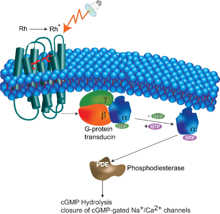
Figure 2: A schematic depiction of the visual signal transduction cascade.

This simple 2-step cascade is commonly embedded in the onset of a reaction pathway of many important signaling cascadespugh92r ; sch02com . For example, the visual signal transduction pathway, which takes place in retinal rod cells, is shown in Fig. 2pugh92r ; bur01act . Rhodopsin receptors (Rh), located in small discs in the outer segments of the rod cell, contain a light-sensitive molecule, retinal. Upon incidence of photons, the retinal molecules undergo isomerization, leading to a subsequent activation of rhodopsin receptors (Rh^∗). The latter act as a catalyst to replace the GDP by GTP in a G-protein, called transducin. The next enzyme in the cascade, the cGMP phosphodiesterase (PDE), is then activated to (PDE^∗) by the active G-protein GTP complex. PDE^∗ hydrolyzes the cGMP, which leads to the closure of cGMP-gated Na⁺/Ca²⁺ ion channels and, thus, reduces the influx of Na⁺/Ca²⁺ flow. The rod cell becomes hyperpolarized, resulting in less neurotransmitters being released from the synaptic terminal of the rod cell. This change is immediately picked up by a second cell and passed as a signal to the central neural system. In this example, the initiating steps of the visual signal transduction pathway,

$$\mbox{Rh}\leftrightarrow\mbox{Rh}^{*}\,,\quad\mbox{G-GDP}+\mbox{Rh}^{*}\leftrightarrow\mbox{G-GTP}+\mbox{Rh}^{*}$$

are similar to our 2-step cascade. The amazing ability of retina rod cells to detect single photons, in the presence of external and internal noise, has been discussed in prior workssch95pht . Although understanding visual signal transduction is not the focus of this work, the formalism of large fluctuations, developed in the current work, may serve as a basis for further elucidating this issue.

We regard the $R\to R^{*}$ reaction (Fig. 1) as a Poisson process with rate $g$, which corresponds to an abundance of $R$ receptors and scarce ligand presence. For instance, the light perception in a dark roomdet00en ; rk98or may be described as a Poissonian bombardment of photons on the retina cell surface. If the intensity of photons is low, there always exist a sufficient excess of inactivated photon receptors ($R$) such that the arrival events of photons dominate the process. $R^{*}$ spontaneously decays back to $R$ at a rate $k$. The average number of activated receptors ($R^{*}$) depends both on the incidence rate $g$ and decay rate $k$. If $R\to R^{*}$ is considered to be an ordinary first order chemical reaction, instead of a Poisson process, all methods described below would still apply, with only minor modifications. Our current investigation is restricted to the $0$-D treatment of space. This is a good approximation if the reaction network is confined to a small enough spatial region, having a linear dimension of $\zeta$ (so-called Kuramoto lengthvan92st ), such that particles diffuse across the region fast compared to the typical reaction times. Using the reaction parameters from published models of the EGF/MAPK signaling cascadesch02com ; thr04dif ; el99prt , we estimated $\zeta$ to be in the range from 0.3 $\mu m$ to 5 $\mu m$. In an ongoing work we are incorporating an explicit treatment of space into our analysis.

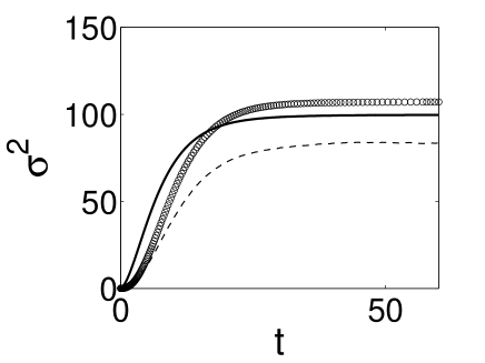
Figure 3: Time evolution of the variance of $A^{*}$ computed from Eq. 1 (solid line), Langevin equation (dashed line) and Eq. 33 (circles). For $(g,k,\mu,\lambda)=(0.2,0.1,0.02,0.15)$ with initial condition $(N_{R},N_{R^{*}},N_{A},N_{A^{*}})=(100,0,100,0)$.

When the number of protein copies in the signaling network is small, the evolution of the averages, described by ordinary chemical kinetics, is inadequate to characterize the system dynamics. An example of the evolution of the $A^{*}$ protein number variance, shown in Figure 3, indicates that the amplitude of the fluctuations is about $10$ in the steady state. This is significant when compared to the deterministic average of about $20$. Clearly, a stochastic description is required in this case. The chemical master equationvan92st is a starting point for studying large variations of individual stochastic trajectories from the average path. For the 2-step cascade described above (Fig. 1), we denote by $P(m,n)$ the probability of having $m$ copies of $R^{*}$ and $n$ copies of $A$ at a particular time point. The time evolution of this probability distribution is determined by the following master equation

$$\frac{dP}{dt}(m,n) = \mu[-mnP(m,n)+m(n+1)P(m,n+1)]+\lambda[-(N-n)P(m,n)$$ (1)

$$+ (N-n+1)P(m,n-1)]+g[-P(m,n)+P(m-1,n)]$$

$$+ k[-mP(m,n)+(m+1)P(m+1,n)]\,,$$

which expresses the transition rates of probabilities from time $t$ to time $t+dt$ in terms of the probability distribution at time $t$. The sum of $A$ and $A^{*}$ is taken to be constant throughout the reaction ($N$ in Eq. (1)). Another way to think about the chemical reaction dynamics given by Eq. (1) is to view it as a random walk on a two-dimensional lattice of integer coordinates $m$ and $n$ with position-dependent jump probabilitiesvan92st .

Since the master equation provides a full description of stochastic chemical process, solutions of the set of coupled ordinary differential equations in Eq. (1) provide all necessary information to analyze the signaling dynamics. However, an exact analytical solution for the system of ODEs in Eq. (1) is not known. Direct numerical integration is also difficult due to the enormous number of ODEs (10⁴-10⁸) for a cascade that may contain up to 10²-10⁴ proteins of each species. Simulations based on the Gillespie algorithm may be used to estimate $P(m,n)$ in Eq. (1), however, they are computationally inefficient and are hard to interpret, as discussed earlier. Thus, to gain qualitative insight into stochastic signal transduction by the 2-step cascade in Fig. 1, it is important to develop an approximate analytical solution to Eq. (1).

Physical considerations are crucially important in making sensible approximations to the master equation. Several numerical and analytical techniques are available to account for the noise effect on signaling dynamics, including the chemical Langevin equation gil00lan and van Kampen’s $\Omega$-expansionvan92st . But they are most useful only when the particle numbers are large and fluctuations are relatively small. In Appendix A we derive an $\Omega$-expansion for the 2-step cascade (1). In the remaining part of the paper, we develop alternative solution schemes to solve equations like Eq. (1), based on the generating function approach, to obtain signaling dynamics in the regime of large fluctuations, where traditional analytical techniques are no longer applicable. Comparison will be made between our method and the results from Langevin equation or $\Omega$-expansion.

Generating function approaches have been used in prior works to elucidate stochastic processes in gene regulatory networksth01in ; sw02in . The novelty of our work is to extend these techniques to nonlinear chemical processes in protein signal amplification cascades. The nonlinearity of chemical reactions greatly enriches the dynamical behavior of signaling cascades. However, to develop a robust analytical approach to solving stochastic amplification dynamics, substantial additional difficulties need to be overcome compared to describing noisy dynamics in linear biochemical networks.

III THE GENERATING FUNCTION APPROACH

To treat signal transduction in a wider range of protein numbers in the cell and to analyze the effects of large fluctuations, we have developed a new approach, based on generating functions, to solve the master equation. A generating function encodes probability distributions as its Taylor series coefficients. As a result, the enormous set of ODEs in Eq. (1) are compactified into a single PDE. Thus, the evolution of the probability distribution can be obtained by solving this one PDE for the generating function. Since even for medium-sized cascades, there are an astronomical number of ODEs in the master equation formalism, an approximate generating function greatly facilitates qualitative and quantitative analysis of strongly-fluctuating dynamics in biochemical reaction networks.

As an example, for the 2-step cascade, we define a generating function through the following power series

$$\Psi(x,y)=\sum_{m,n}P(m,n)x^{m}y^{n}\,.$$ (2)

which satisfies the time evolution equation

$$\frac{\partial\Psi}{\partial t}=(1-y)(\mu x\frac{\partial^{2}}{\partial x\partial y}-\lambda N+\lambda y\frac{\partial}{\partial y})\Psi+g(x-1)\Psi-k(x-1)\frac{\partial\Psi}{\partial x}\,.$$ (3)

Our next goal is to develop approximate techniques to solve Eq. (3). We know that the solution of Eq. (3) is an analytic function of $x\,,y$ with nonnegative time-dependent coefficients. The highest derivative in Eq. (3) is $\partial^{2}\Psi/\partial x\partial y$ which reflects the binary chemical reaction between $R^{*}$ and $A$. If this term is omitted, Eq. (3) can easily be solved by the method of characteristics. However, this would completely alter its physical content. On the other hand, we notice that the generating function of the $R^{*}$ distribution $\phi(x)=\Psi(x,1)$ does not depend on the dynamics of $A$ and obeys the following PDE

$$\frac{\partial\phi}{\partial t}=g(x-1)-k(x-1)\frac{\partial\phi}{\partial x}\,,$$ (4)

which can be solved exactly, resulting in

$$\phi(x)=\exp[\frac{g}{k}(x-1)(1-e^{-kt})]\,,$$ (5)

where the initial condition $N_{R^{*}}=0$ at $t=0$ was used. The $R^{*}$ probability distribution, $P(m)$, is given by the coefficients of the series expansion of Eq. (5)

$$\phi(x)=\sum_{m=0}^{\infty}\exp(-\frac{g}{k}(1-e^{-kt}))(1-e^{-kt})^{m}(\frac{g}{k})^{m}\frac{x^{m}}{m!}$$ (6)

resulting in,

$$P(m)=\exp(-(1-e^{-kt})g/k)(1-e^{-kt})^{m}(\frac{g}{k})^{m}/m!\,.$$ (7)

Therefore, the time-dependent distribution of $R^{*}$ is Poissonian and relaxes to a stationary distribution with the rate $k$. Although this distribution is generated by both the birth and decay of $R^{*}$, the relaxation is independent of birth rate $g$. From Eq. (6), the average and the variance of $N_{R^{*}}$ are also easily calculated, $\langle N_{R^{*}}\rangle=\langle\sigma^{2}\rangle=(1-e^{-kt})g/k$.

Next, we build up the cascade by considering also the reactions involving $A$. In particular, we construct a series expansionince in $x$ with time-dependent functions $\phi_{m}(y)$,

$$\Psi(x,y)=\sum_{m=0}^{\infty}\phi_{m}(y)x^{m}\,.$$ (8)

Thus, with each state containing $m$ $R^{*}$’s, we associate a distribution of $A$, which may be computed from $\phi_{m}(y)$. The new functions $\phi_{m}(y)$ satisfy

$$\frac{\partial\phi_{m}}{\partial t}=(1-y)(\mu m\frac{\partial}{\partial y}-\lambda N+\lambda y\frac{\partial}{\partial y})\phi_{m}+km(\phi_{m+1}-\phi_{m})+g(\phi_{m-1}-\phi_{m})+k\phi_{m+1}\,.$$ (9)

Here an infinite hierarchy of coupled linear PDEs are obtained for the unknown functions $\phi_{m}(y)$. Eq. (9) is exactly equivalent to the master equation and physical considerations will next be used in finding good-quality approximate solutions. We start by keeping only the first term in Eq. (9), thus, ignoring the $R\to R^{*}$ dynamics, and then incorporate back the omitted terms in an effective way.

III.1 Time-scale separation modulates noise propagation

The first term on the right hand side of Eq. (9) describes the birth and death of protein $A$ and the remaining terms describe $R^{*}$ dynamics. If the $R^{*}$ reaction is ignored, the hierarchy of PDEs become uncoupled. We obtained an exact analytical solution for the resulting PDEs using the method of characteristics:

$$\phi_{m}^{(0)}(y)=\phi_{m,0}[1+\left(\frac{\lambda}{\lambda+\mu m}+\frac{\mu m}{\lambda+\mu m}e^{-(\lambda+\mu m)t}\right)(y-1)]^{N}\,,$$ (10)

where the number of $A$’s was taken to be $N$ at $t=0$ and $\phi_{m,0}$ is a constant, representing the probability of having exactly $m$ $R^{*}$’s. If, for example, the number $m$ of $R^{*}$ is fixed at a particular value $\bar{m}$, then $\phi_{\bar{m},0}=1\,,\phi_{m}=0$ for $m\neq\bar{m}$. The obtained generating function indicates that the $A$ distribution is binomial. Note that the relaxation rate is $\lambda+\mu\bar{m}$, depending on both $\lambda$ and $\mu$. The solution further simplifies in the limit of long times ($t\to\infty$).

$$\phi_{\bar{m}}^{(0)}\to\phi_{\bar{m},0}[1+\frac{\lambda}{\lambda+\mu\bar{m}}(y-1)]^{N}\,,$$ (11)

which is the generating function for the stationary distribution of $A$.

In the real 2-step biochemical cascade, the number of $R^{*}$’s is, of course, fluctuating. However, Eq. (10), with $m$ concentrated at $\bar{m}$, still constitutes a good approximation when either of the following conditions is satisfied: (i) $R^{*}$ is characterized by a sharp distribution centered at $\bar{m}$, which is often the case when the number of $R^{*}$’s is large; (ii) the reaction rates for $R^{*}$ birth and death are much larger than those for $A$. For a cascade that satisfies condition (i), the linear noise approximation might be applicable. However, our solution, based on the generating function approach, provides the full probability distribution in an analytical form. When condition (ii) is satisfied, the $A\to A*$ reaction only “sees” an average number ($\bar{m}$) of $R^{*}$. In this case, our solution is simpler and, perhaps more convenient to use, than the $\Omega-$expansion solution. Analysis of the cascade dynamics for case (ii) using Eq. (10) suggested a possible mechanism for noise filtering. Even in the case of broad or irregular distribution for $R^{*}$, if the fluctuations around the average are fast, the distribution of $A$ is still well approximated by Eq. (10), being well-peaked at the average for large $N$.

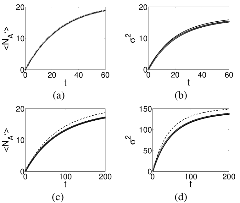
Figure 4: Time evolution of the averages ((a) and (c)) and variances ((b) and (d)) for $A^{*}$ obtained from three different calculations: the approximate solution Eq. (10) (circles), the exact solution (solid line computed from Eq. (1)) and the $\Omega$-expansion Eq. (33) (dashed line probably overlapped by the solid line). The initial condition is $(N_{R},N_{R^{*}},N_{A},N_{A^{*}})=(100,0,100,0)$. (a) and (b) have parameter values $(g,k,\mu,\lambda)=(20,10,0.004,0.03)$; (c) and (d) have parameter values $(g,k,\mu,\lambda)=(0.02,0.01,0.2,1.5)$.

As an example, we take the reaction rate parameter values $(g,k,\mu,\lambda)=(20,10,0.004,0.03)$ and initial condition $(N_{R},N_{R^{*}},N_{A},N_{A^{*}})=(100,0,100,0)$. The evolution of the first two moments of $N_{A^{*}}$ as computed from our approximate solution Eq. 10, $\Omega-$expansion solution Eqs.32,33, and exact numerical results are shown in Fig. 4a,b. Unlike the practical implementation of the $\Omega-$expansion, Eq. 10 also directly gives the time evolution of the full probability distribution for $A^{*}$ proteins. A time slice of the probability distribution of $A^{*}$ is shown in Fig. 5a. Overall, a remarkable agreement is achieved between the approximate analytical results and exact numerical calculations. Also shown in the figure is the distribution computed from the Langevin equation (dashed line), which is characterized by an average noticeably larger than the exact average. Even though the magnitude of $R^{*}$ fluctuations is the same for the cascade parameters used in Figs. 3,4,5, the $A^{*}$ fluctuations are dramatically attenuated for the case demonstrated in Fig. 4b and 5a, compared with Fig. 3. In this case the $R\to R^{*}$ reactions are much faster than the $A\to A^{*}$ reactions, thus, the $R\to R^{*}$ noise is averaged out and only internal $A\to A^{*}$ noise remains. If we think of this two-step cascade as an element of a longer signaling pathway, the relatively large fluctuations of the upstream reaction ($R\to R^{*}$) become attenuated downstream ($A\to A^{*}$). Thus, stacking of a slow downstream reaction after a fast upstream reaction provides a general mechanism for noise attenuation in biochemical signaling networks.

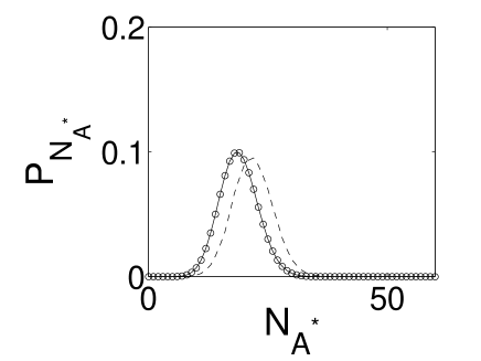
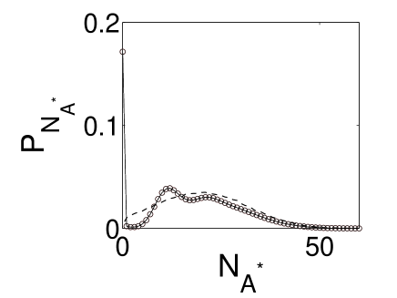
Figure 5: Probability distributions of $A^{*}$ computed from the approximate solution Eq. 10 (circles), Langevin equation (dashed line) and the exact solution Eq. 1 (solid line) with initial condition $(N_{R},N_{R^{*}},N_{A},N_{A^{*}})=(100,0,100,0)$. (a) The distribution $P(N_{A^{*}})$ at $t=60$ with parameter values $(g,k,\mu,\lambda)=(20,10,0.004,0.03)$. (b) The distribution $P(N_{A^{*}})$ at $t=200$ with parameter values $(g,k,\mu,\lambda)=(0.02,0.01,0.2,1.5)$.

In the opposite limit of the reaction rate of $R^{*}$ being much slower than that of $A$, we can take into account the $R^{*}$ dynamics by allowing $\phi_{m,0}$ in Eq. (10) to change slowly with time according to Eq. (7). Thus, we substituted

$$\phi_{m,0}=\exp(-(1-e^{-kt})g/k)(1-e^{-kt})^{m}(\frac{g}{k})^{m}/m!\,.$$ (12)

into Eq. (10). This is a valid approximation in the limit of slow $R^{*}$ dynamics. Using this substitution, we obtained an approximate solution for $\Psi(x,y)$ as an infinite sum over the $R^{*}$ protein number $m$. Since the coefficients of $x^{m}$ decay very fast with increasing $m$, we can safely truncate it to a finite sum. For many reaction rates in this regime, the obtained distribution is broad.

A set of reaction rates, which corresponds to a slow upstream reaction and a fast downstream reaction $(g,k,\mu,\lambda)=(0.02,0.01,0.2,1.5)$, was used to compare our analytical calculations with exact numerical results (Fig. 4c,d and Fig. 5b). The evolution of both the first moment (Fig. 4c) and the variance (Fig. 4d) obtained from our analytical treatment agrees well with the exact numerical one, being more accurate than the $\Omega$-expansion. Furthermore, we used Eq. 8, Eq. 10, and Eq. 12 to compute the full probability distribution at $t=200$ (Fig. 5b), which is impossible to obtain analytically using the $\Omega$-expansion approach. All the nuances of the complicated distribution are accurately captured by our approximate analytic solution. The distribution computed from the Langevin equation, on the other hand, which is shown as a dashed line in Fig. 5b, is characterized by a single broad peak. The white noise terms in the Langevin equation obviously smear out the peaks and, thus, are not good models for the underlying stochastic dynamics. At long time limits the distribution becomes uni-modal, but still wide (data not shown).

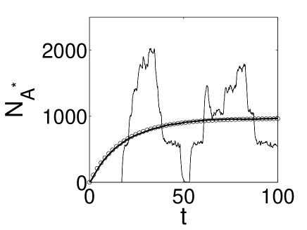
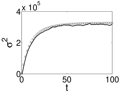
Figure 6: (a) Averages computed from Gillespie simulation (solid line) and from the approximate solution Eq. (8) (circles). One typical Gillespie trajectory is also shown (thin solid line); (b) the variance from Gillespie simulation (solid line) and from the approximation (circles). Initial condition $(N_{R},N_{R^{*}},N_{A},N_{A^{*}})=(100,0,5000,0)$ and parameter values $(g,k,\mu,\lambda)=(0.1,0.05,0.2,1.5)$.

The fluctuations in $A^{*}$ are much larger for a cascade where the upstream reaction is slow and the downstream reaction is fast (Fig. 4d and Fig. 5b) compared with previously considered cascades (Figs. 3, 4b and 5a). Thus, the noise produced in the $R\to R^{*}$ reaction is retained and amplified by the next enzymatic reaction. As opposed to the previously discussed case of noise-attenuation, this cascade setup could be used to amplify the noise downstream. The amplification and attenuation of noise have been extensively discussed and experimentally tested in the linearized stochastic description of gene regulatory networksth01in ; kie01eff ; oz02reg ; bla03noi . Our current work emphasizes the role of discreteness in a nonlinear biochemical reaction network, using directly the generating function formalism to obtain analytical time-dependent probability distributions.

Strong fluctuations occur even when the number of downstream proteins is very large. Fig.  6 demonstrates a striking example. Although the average number of $A^{*}$ quickly reaches its steady-state value, which is near $1000$, the fluctuation continues, such that a typical trajectory fluctuates with a magnitude of the same order as the average (Fig. 6a). The corresponding large variance, shown in Fig. 6b, confirms this analysis. Thus, the fluctuations are much larger than expected from the usual $\sqrt{N}$ argument, where N is the number of proteins. Our approximate solution agrees very well with the exact solution (Fig. 6), confirming the validity of our noise-amplification scheme to solve the master equation (Eqs. (8), (10) and (12)). The large $A^{*}$ fluctuations are induced by the upstream $R^{*}$ fluctuations, as seen from a typical numerical trajectory shown in Fig.6a. At steady state, the average death/birth timescale for $R^{*}$ is $1/g=10$, thus, the $A^{*}$ trajectory exhibits a bursting behavior with a time correlation of about $10$.

In the photoreception cascade, the rhodopsin (Rh) activation is controlled by the incident photons which may arrive, one by one, within $1s$ or even longer time interval in the single photon experimentsch95pht . The deactivation rate from Rh^∗ to Rh is about $0.5s^{-1}$. The activation rate of the transducinbur01act is around $120s^{-1}$ and the deactivation rate is $100s^{-1}$. According to the classification developed in this paper, the initiating stage of the photoreception cascade belongs to the case of slow $R^{*}$ reaction and fast $A$ reaction, thus, we expect an amplification of the external light stimulation sch95pht ; rk98or ; bur01act .

Our approximation method in this section is based on the separation of time scales for the first and the second reactions, an approach which is also the starting point for many solution techniques in the literature. The elimination of fast variables is among the most popular ones and is often used to approximately solve Fokker-Planck or Langevin equations van92st ; gar02han . Various methods such as the projection operator method gar02han and cumulant expansion method van92st have been developed to treat the continuous cases. To the lowest order approximation, the fast time scale is completely removed, while the equations for the slow variables account for the fast variables either through their corresponding averages van92st or through their stationary distributions gar02han . Here we applied the essence of this idea to the discrete jump process described by a master equation and obtained analytical approximations for the evolving probability distribution function. Similar consideration has been used to derive effective equations in gene transcription regulation in the large particle limit th01st , but our method applies to small particle numbers as well. In the first case considered above (fast $A-A^{*}$ reaction), we used only the average of the fast variable. In the second case (fast $R-R^{*}$ reaction), we first considered the probability distribution evolution of the fast variable and, subsequently, incorporated back the evolution of the slow variable. Thus, in both cases, we explicitly included both the slow and fast time scales into the final analytical expression.

IV Solving the master equation with the hybrid smooth probability distribution method

When the probability distributions are relatively smooth, a new approximation scheme may be employed to integrate the generating function equation 3. To show basic idea of the method, we first implement it for the 2-step cascade discussed previously (Fig. 1). Then, to demonstrate the potential for generalization, we apply this method to another enzymatic cascade, where the first step is a self-dimerization of receptor $R$ instead of a simple activation.

IV.1 2-step signal transduction cascade

To treat analytically the stochastic signaling dynamics in a wider regime of parameters (for example, when upstream and downstream reactions have comparable rates), the neglected coupling terms in Eq.9 may be taken into account in a more systematic way. In this section, we will reconsider the cross terms between different $m$’s and treat them in a different way. Here, we take advantage of the known $R^{*}$ distribution from Eq. 6 and write down the following expansion for $\Psi(x,y)$,

$$\Psi(x,y)=\sum_{m=0}^{\infty}\exp(-\frac{g}{k}(1-e^{-kt}))(\frac{g}{k})^{m}\frac{x^{m}}{m!}\phi_{m}(y)\,,$$ (13)

where $\phi_{m}(y)$ is a time-dependent function and, according to Eq. (6), we know that $\phi_{m}(1)=(1-e^{-kt})^{m}$. Substituting this form of expansion of $\Psi$ into Eq. (3) and comparing the coefficient of $x^{m}$ on both sides of the equation, we have

$$\frac{\partial\phi_{m}}{\partial t}=(1-y)(\mu m\frac{\partial}{\partial y}-\lambda N+\lambda y\frac{\partial}{\partial y})\phi_{m}+km(\phi_{m-1}-\phi_{m})+g(\phi_{m+1}-\phi_{m})+ge^{-kt}\phi_{m}\,.$$ (14)

This equation describes the time evolution of $\phi_{m}(y)$, which is coupled to the neighboring functions $\phi_{m-1}$ and $\phi_{m+1}$. In previous discussions, we neglected these couplings first and only later incorporated them back in an effective way, justified under certain conditions. Here, we present an approach which directly takes into account these couplings in an approximate manner. When the probability distribution of $R^{*}$is smooth, the following approximation,

$$\frac{\partial\phi_{m}}{\partial m}\approx\phi_{m+1}-\phi_{m}\approx\phi_{m}-\phi_{m-1}\,,$$ (15)

may be used to uncouple the PDEs in Eq. (14):

$$\frac{\partial\phi_{m}}{\partial t}=(1-y)(\mu m\frac{\partial}{\partial y}-\lambda N+\lambda y\frac{\partial}{\partial y})\phi_{m}+(g-km)\frac{\partial\phi_{m}}{\partial m}+ge^{-kt}\phi_{m}\,,$$ (16)

We solved the resulting PDEs by the method of characteristics. Eq. (15) is satisfactory when the profile of $\phi_{m}$ between $m$ and $m+1$ can be reasonably approximated by a straight line segment. This works well if either of the two conditions holds: (1) as mentioned above, the distribution profile is smooth so that the higher-order derivatives can be ignored, or (2) the number of $R^{*}$ is large such that an increment by one particle may be treated as small. In addition, it is possible to improve this solution by making a higher-order approximation to the difference in Eq. (15). For example, an exact expression can be obtained through the Kramers-Moyal expansiongar02han

$$\phi_{m+1}-\phi_{m}=\sum_{l}\frac{1}{l!}\frac{\partial^{l}}{\partial m^{l}}\phi_{m}\,,$$

where $l$ runs from $1$ to $\infty$. In the standard derivation of the Fokker-Planck equationvan92st ; gar02han , terms up to the second order ($l=2$) are retained. In some sense, our “smooth distribution” method is a hybrid distribution function – generating function scheme, where in the yet to be determined functions $\phi_{m}(y)$, subscript $m$ is related to the $R^{\star}$ particle number (distribution for $m$), while $y$ is a formal variable related to the generating function for the $A^{\star}$ particle number. However, solving equations containing higher-order derivative terms quickly becomes cumbersome. Here, we only keep the first order term, which allows Eq. (16) to be solved with the following set of characteristic equations

$$\dot{y} = (y-1)(\mu m+\lambda y)$$

$$\dot{m} = mk-g$$

$$\dot{\phi_{m}} = \lambda N(y-1)\phi_{m}+ge^{-kt}\phi_{m}\,.$$ (17)

The first two equations in Eq. (17) define the characteristic curves and the third equation shows how $\phi_{m}$ changes along this curve. The dynamics on each curve is self-contained and independent of each other, which is the consequence of neglecting higher order terms in Eq. (15). Eq. (17) were exactly solved, resulting in

$$\phi_{m}(y)=\phi_{m}^{(0)}(z_{0})(1+\frac{\lambda p}{p^{\prime}}(y-1))^{N}\exp[\frac{g}{k}(1-e^{-kt})]\,,$$ (18)

where

$$\phi_{m}^{(0)} = \sum_{n=0}^{N}a_{nm}(\frac{1}{z_{0}}+1)^{n}$$

$$z_{0} = \frac{p^{\prime}}{y-1}+\lambda p$$

$$p(t) = \int_{0}^{t}e^{I(s)}ds$$

$$I(t) = (\lambda+\frac{\mu g}{k})t+\frac{\mu}{k}(m_{0}-\frac{g}{k})(e^{kt}-1)\,.$$

$a_{nm}$ is the initial probability of having $m$ $R^{*}$’s and $n$ $A$’s and $m_{0}$ is an intermediate variable which after all the integrations and differentiations are done will be replaced by $m$ by the following substitution,

$$m_{0}-\frac{g}{k}=(m-\frac{g}{k})e^{-kt}\,.$$ (19)

In general, the integration to obtain $p(t)$ can not be carried out in a closed form, thus, approximate or numerical treatment is needed. However, the analytic structure of the overall solution is transparent. The last exponential factor in Eq. (18) describes the $R^{*}$ reaction and the first two factors describe the $A\to A^{*}$ reaction. The full generating function $\Psi(x,y)$ is given by Eq. (13) with $\phi_{m}(y)$ given by Eq. (18). Once $\Psi(x,y)$ is known, all the statistical quantities are easily computable.

As an example, we consider the following initial distribution

$$\phi_{m}^{(0)}=e^{-m}(\frac{1}{z_{0}}+1)^{N}\,,$$ (20)

which corresponds to starting the cascade dynamics with $N$ $A$’s and a small number of $R^{*}$, distributed exponentially. The corresponding solution is given by

$$\phi_{m}(y)=(1+\frac{\lambda p+1}{p^{\prime}}(y-1))^{N}\exp(-me^{-kt})\,,$$ (21)

where

$$p^{\prime}(t) = \exp((\lambda+\frac{\mu g}{k})t+\frac{\mu}{k}(m-\frac{g}{k})(1-e^{-kt}))$$

$$p(t) = \int_{0}^{t}\exp((\lambda+\frac{\mu g}{k})s+\frac{\mu}{k}(m-\frac{g}{k})(e^{k(s-t)}-e^{-kt}))\,ds\,.$$ (22)

When $x=1$, if the following approximation is used

$$\phi_{m}=\exp(-me^{-kt})\approx(1-e^{-kt})^{m}\,,$$ (23)

then the $R^{*}$ distribution is recovered. Furthermore, Eq. (21) with Eq. (23) substituted in conserves the total probability, i.e., $\Psi(1,1)=1$. Thus, we use Eq. (23) in the calculations described below.

To gauge the effectiveness of the approximate analytical solution, we take $N=100$ and the $R^{*}$ distribution truncated at $m=30$. Firstly, we evaluate Eq. (21) with $(g\,,k\,,\mu\,,\lambda)=(10\,,1\,,0.01\,,0.1)$. $A^{*}$ distribution computed from Eq. (13) at $t=60$ matches quite well with the exact solution as shown in Fig. 7a. The approximate distribution is a little narrower than the exact one due to the omission of the higher-order derivative terms in Eq. (15). Secondly, we carried out similar calculations with $(g\,,k\,,\mu\,,\lambda)=(0.2\,,0.1\,,0.02\,,0.2)$, as shown in Fig. 7b. Although the distribution at $t=60$ from our approximation agrees quite well with the exact solution for large $N_{A^{*}}$, near the left boundary there is a clear discrepancy, due to the non-smoothness of the distribution at the minimum particle number, since the number of $A^{*}$ cannot be negative.

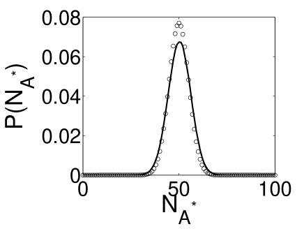
(a) The distributions at $t=6$

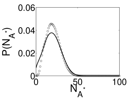
(b) The distributions at $t=60$

Figure 7: The probability distributions of $A^{*}$ at $t=60$ computed from the approximate solution Eq. (21) (circles) and the exact solution Eq. (1) (solid line) with initial condition $(N_{R},N_{R^{*}},N_{A},N_{A^{*}})=(100,0,100,0)$ and parameter values: (a) $(g\,,k\,,\mu\,,\lambda)=(10\,,1\,,0.01\,,0.1)$; (b) $(g\,,k\,,\mu\,,\lambda)=(0.2\,,0.1\,,0.02\,,0.2)$.

IV.2 Receptor self-dimerization introduces additional nonlinearity

Even if the exact solution is not available for the first reaction, we can still apply the above approximation as long as the distribution is smooth. Consider the dimerization reaction shown in Fig. 8. Compared to the previously discussed 2-step cascade (Fig. 1), the first reaction is replaced by a self-dimerization process with rate $g$. This dimerization activation is quite common in signal transduction and gene regulatory networks jas04fl ; bun03fl ; hay04lin . Although it is possible to derive an analytical solution for the isolated first step in the cascade, i.e. the self-dimerization process nic77self ; rei98st , the expression is in a series form and will not be used in our approximation scheme.

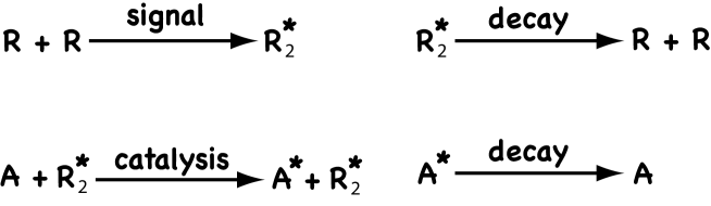
Figure 8: An inactive receptor $R$, when activated by dimerization, activates downstream protein $A$.

Again, let $P(m,n)$ denote the probability of having $m$ $R_{2}^{*}$’s and $n$ $A$’s. The master equation is then,

$$\frac{dP}{dt}(m,n) = \frac{g}{2}\left((M-2m+2)(M-2m+1)P(m-1,n)-(M-2m)(M-2m-1)P(m,n)\right)$$ (24)

$$+k\left((m+1)P(m+1,n)-mP(m,n)\right)+\mu\left((n+1)mP(m,n+1)-mnP(m,n)\right)$$

$$+\lambda\left((N-n+1)P(m,n-1)-(N-n)P(m,n)\right)\,,$$

where the first term describes the dimerization reaction. The corresponding generating function $\Psi(x,y)$ satisfies,

$$\frac{\partial\Psi}{\partial t} = \frac{g}{2}(x-1)\left(M(M-1)+4x^{2}\frac{\partial^{2}}{\partial x^{2}}-2(2M-3)x\frac{\partial}{\partial x}\right)\Psi$$ (25)

$$+k(1-x)\frac{\partial\Psi}{\partial x}+\mu(1-y)x\frac{\partial^{2}\Psi}{\partial x\partial y}+\lambda(y-1)(N-y\frac{\partial}{\partial y})\Psi\,.$$

Note that a new second-order derivative, $\partial^{2}\Psi/\partial x^{2}$, appears, compared with the previously considered generating function PDE (Eq. (3)). If we expand the generating function in the form of Eq. (8), a series of PDEs for $\phi_{m}$’s are derived. Similar to the simple 2-step cascade, after taking the continuous limit approximation, we get

$$\frac{\partial\phi_{m}}{\partial t} \approx (1-y)(\mu m\frac{\partial}{\partial y}-\lambda N+\lambda y\frac{\partial}{\partial y})\phi_{m}$$ (26)

$$+\frac{\partial}{\partial m}\left(km-\frac{g}{2}(M(M-1)+4m(m-1)-2(2M-3)m)\right)\phi_{m}\,,$$

where the total probability is conserved since

$$\frac{d}{dt}\int_{-\infty}^{\infty}dm\,\phi_{m}(t,1)=0\,.$$

Eq. (26) are also readily solved analytically by the characteristic method.

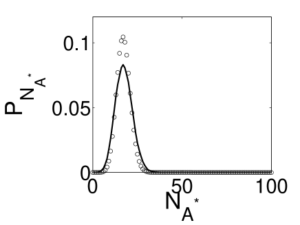
(a) The distribution at t=3

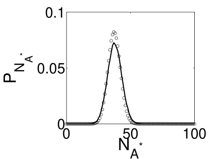
(b) The distribution at t=60

Figure 9: Probability distributions of $A^{*}$ computed from the approximate solution Eq. 26 (circles) and Gillespie simulation (solid line) averaged over $70898$ realizations. Initially $(N_{A},N_{A^{*}})=(100,0)$ and $N_{R_{2}^{*}}$ approximately assumes a Gaussian distribution $\exp(-(m-2)^{2})/\sqrt{\pi}$. We use $N_{R}+2N_{R_{2}^{*}}=20$ and choose parameter values $(g,k,\mu,\lambda)=(0.02,0.5,0.02,0.15)$. (a) The distribution $P(N_{A^{*}})$ at $t=3$. (b) The distribution $P(N_{A^{*}})$ at $t=60$.

The approximate distributions compared with those computed from Gillespie simulation are displayed in Fig. 9 at an early time $t=3$ and a later time $t=60$. They agree quite well. The approximate and exact distributions at other times are in good agreement as well (data not shown).

Overall, the presented method may be used to obtain the long time evolution of the stochastic signaling dynamics. We designed the hybrid scheme to treat the second order derivative terms in the generating function equation with the characteristics method. When the probability distribution profiles of all species are relatively smooth the method gives quantitatively accurate results. Although, this condition is most commonly satisfied when protein numbers are large, it is also applies to systems with smaller protein numbers with certain constraints on the relative reactions rates. Generalizing this method to treat larger cascades is also straightforward. If all the reaction nodes in the network are linear, then there is no need to expand the generating function equation up to second order derivative terms, and a direct application of the characteristics method would solve the generating function PDE. If a small number of binary reaction nodes are present, the hybrid scheme can be applied most effectively, allowing to obtain approximate solutions in a manner similar to the examples that we have already considered. For cascades with many binary reactions, a straightforward application of the method may becomes unpractical since a summation over many indices is required, which would be computationally expensive. However, this difficulty may be overcome by either linearizing the nonessential binary terms or by approximating the summations with integrals.

V Conclusions

Cells live in a fluctuating environment in which signals and noise keep bombarding the cell receptorsst02gomp ; bar98bac ; sm05inf . Noisy signals propagate inside the cell via microscopic chemical reaction events. The external noise interferes with the internal biochemical network noise originating from the underlying fundamental randomness of these chemical reactions. Cells have evolved to adapt to or even exploit the seemingly deleterious effect of fluctuations on signaling dynamics within a mesoscopic size object. Thus, it is important to develop a qualitative picture, based on mathematical modeling of stochastic chemical kinetics, of how signaling networks process noisy signals. In this paper we studied the stochastic signal transduction by a simple 2-step signaling cascade using the master equation to describe stochastic reaction events. In agreement with previous studies, we found that when particle numbers are large, chemical kinetic equations provide an accurate description. However, when the number of proteins becomes small, a large variability among individual trajectories results, necessitating the stochastic chemical kinetics approach. If fluctuations are small, the commonly used linear noise approximation works well, the probability distribution being centered around the deterministic trajectory. But when fluctuations are large, for example, at the initiating (burst) phase of a signal transduction cascade, the linear noise approximation breaks down and more powerful analytical treatment of the master equation becomes necessary. In the small protein number regime, chemical Langevin equation does not work properly as well since the continuous assumption breaks down and molecular discreteness sets in the dynamics.

Without assuming that noise is small, we directly treated the master equation with a generating function approach. Although the resulting PDE could not be solved exactly, we found a number of perturbative schemes, that allow us to obtain approximate analytic solutions for the generating function which is used to obtain the time evolution of the full probability distribution for all proteins. Using the analytic solution, we recovered the general mechanism for attenuating or amplifying noise in a signaling pathway with nonlinear reaction events: if the upstream reactions are fast and the downstream reactions slow, then upstream noise becomes attenuated. Conversely, if the upstream reactions are slow and the downstream reactions fast, then the upstream noise becomes amplified. Thus, controlling various node timescales by regulating reaction rate constants would lead to enhancing of the signaling cascade sensitivity and reliability by suppressing uncorrelated noise while still amplifying weak signals. This mechanism may be used by cells to draw useful information from a noisy environment. Furthermore, under certain conditions, the burst phase noise may induce macroscopic system-wide disturbance in the downstream signaling network.

The approximation based on characteristics, presented in Section IV, can be straightforwardly generalized to a longer cascade, with the restriction that the protein number distributions are smooth. Yet another powerful technique to solve the master equation for more complex cascades is based on the variational principle eyink96act . The analytic solutions developed in this paper serve as a starting point for developing high quality time-dependent basis sets for the variational approach. A good basis set should capture the essential part of the system dynamics so as to make the subsequent calculations simple and effective, which will be discussed in more detail elsewhere. For larger signaling pathways, especially when embedded in space, the commonly used numerical stochastic simulations will face severe computational bottleneck. In this work we have taken a different approach, based on analytically solving the master equation describing stochastic chemical kinetics, to achieve, in an efficient manner, qualitative and quantitative insights into stochastic signaling by biochemical reaction networks. In an ongoing work we are generalizing the techniques presented in this work to investigate the interplay of the noise amplification and attenuation with the complex dynamics generated from feedback loops in larger biochemical reaction networks.

Appendix A: The $\Omega$-expansion of the 2-step cascade master equation

If the fluctuations are relatively small, van Kampen’s $\Omega$-expansion may be used to account for their effect on signaling dynamicsvan92st . In this case it is more convenient to rewrite the master equation, given by Eq. 1, in an alternative formvan92st , where the dependence of reaction rates on the cell size, $\Omega$, is explicitly emphasized:

$$\dot{P}=\lambda(E_{n}^{-1}-1)(N-n)P+\frac{\mu}{\Omega}(E_{n}^{+1}-1)mnP+k(E_{n}^{+1}-1)mP+g\Omega(E_{n}^{-1}-1)P\,,$$ (27)

where $E_{n}^{+1}f(n)=f(n+1)$ and $E_{n}^{-1}f(n)=f(n-1)$ are step-up and step-down operatorsvan92st . Although $\Omega$ is equal to 1 in our units, it is still written out to be used later as an expansion parameter. If the protein numbers are large enough such that the deterministic evolution serves as a good starting point, then small fluctuations are well described by the linear noise approximation. In particular, the variables are changed to emphasize the fluctuations around the deterministic orbits:

$$m = \Omega\phi(t)+\Omega^{1/2}\xi\,,$$

$$n = \Omega\psi(t)+\Omega^{1/2}\eta\,,$$

$$P(m,n,t) = \Pi(\xi,\eta,t)\,,$$

$$N = \bar{N}\Omega\,.$$ (28)

where $\phi(t)$ traces the deterministic path for $N_{R^{*}}$ and $\psi(t)$ for $N_{A}$. The new random variables are $\xi$ and $\eta$, that describe fluctuations around the average path. While averages determined from the dominant paths are proportional to $\Omega$, fluctuations around these averages are only proportional to $\Omega^{1/2}$. Since $\phi(t)$ and $\psi(t)$ can be easily found by solving the chemical kinetic equation, we need to obtain an evolution equation for the probability distributions of $\xi$ and $\eta$, $\Pi(\xi,\eta,t)$. Thus, we substitute Eq. 28 into Eq. 27, using also the following expression for any analytic function $f(n)$:

$$(E_{n}^{\pm 1}-1)f(n)=(\pm\frac{\partial}{\partial n}+\frac{1}{2}\frac{\partial^{2}}{\partial n^{2}}+\dots)f(n)\,.$$

Eq. 27 results in

$$\frac{\partial\Pi}{\partial t}-\Omega^{1/2}\frac{d\phi}{dt}\frac{\partial\Pi}{\partial\xi}-\Omega^{1/2}\frac{d\psi}{dt}\frac{\partial\Pi}{\partial\eta}=\lambda(-\Omega^{-1/2}\frac{\partial}{\partial\eta}+\frac{1}{2}\Omega^{-1}\frac{\partial^{2}}{\partial\eta^{2}})(\Omega(\bar{N}-\Psi)-\Omega^{1/2}\eta)\Pi$$

$$+\frac{\mu}{\Omega}(\Omega^{-1/2}\frac{\partial}{\partial\eta}+\frac{1}{2}\Omega^{-1}\frac{\partial^{2}}{\partial\eta^{2}})(\Omega\phi+\Omega^{1/2}\xi)(\Omega\psi+\Omega^{1/2}\eta)\Pi+k(\Omega^{-1/2}\frac{\partial}{\partial\xi}+\frac{1}{2}\Omega^{-1}\frac{\partial^{2}}{\partial\xi^{2}})$$

$$(\Omega\phi+\Omega^{1/2}\xi)\Pi+g(-\Omega^{-1/2}\frac{\partial}{\partial\xi}+\frac{1}{2}\Omega^{-1}\frac{\partial^{2}}{\partial\xi^{2}})\Omega\Pi+\cdots\,.$$ (29)

We next collect terms that are of the same order in $\Omega$. The largest $\Omega^{1/2}$ terms give:

$$-\frac{d\phi}{dt}\frac{\partial\Pi}{\partial\xi}-\frac{d\psi}{dt}\frac{\partial\Pi}{\partial\eta}=-\lambda(\bar{N}-\psi)\frac{\partial\Pi}{\partial\eta}+\mu\phi\psi\frac{\partial\Pi}{\partial\eta}+k\phi\frac{\partial\Pi}{\partial\xi}-g\frac{\partial\Pi}{\partial\xi}\,,$$

which is satisfied as we choose the dynamics of $\phi$ and $\psi$ to follow chemical kinetics

$$\frac{d\phi}{dt} = g-k\phi\,,$$

$$\frac{d\psi}{dt} = \lambda(\bar{N}-\psi)-\mu\phi\psi\,.$$ (30)

At the $\Omega^{0}$ order, we obtain

$$\frac{\partial\Pi}{\partial t}=\lambda\frac{\partial}{\partial\eta}(\eta\Pi)+\mu\frac{\partial}{\partial\eta}(\xi\psi+\eta\phi)\Pi+k\frac{\partial}{\partial\xi}(\xi\Pi)+\frac{1}{2}(\lambda(\bar{N}-\psi)+\mu\phi\psi)\frac{\partial^{2}\Pi}{\partial\eta^{2}}+\frac{1}{2}(k\phi+g)\frac{\partial^{2}\Pi}{\partial\xi^{2}}\,,$$ (31)

which is the familiar Fokker-Planck equation, derived in a systematic way. Eq. 31 is the linear noise approximation to the full stochastic dynamics, which is valid when the path determined by Eq. 30 is stablevan92st . Eq. 31 is a linear PDE that has to be solved numerically. However, it is possible to derive a closed set of ODEs to describe time evolutions of the moments up to any order. For example, the averages (first moments) satisfy

$$\frac{d\langle\eta\rangle}{dt} = -(\lambda+\mu\phi)\langle\eta\rangle-\mu\psi\langle\xi\rangle$$

$$\frac{d\langle\xi\rangle}{dt} = -k\langle\xi\rangle\,,$$ (32)

which are just the linearized chemical kinetics equations. Note that if initial values of $\langle\eta\rangle$ and $\langle\xi\rangle$ are taken to be zero, then they remain zero for all later times, consistent with the physical significance of Eq. 30 which describes the evolution of averages of protein numbers. This also suggests that application of Eq. 31 is based on the assumption of the validity of averaged chemical kinetics equations. Next, we consider three second moments, satisfying

$$\frac{d\langle\eta^{2}\rangle}{dt} = -2(\lambda+\mu\phi)\langle\eta^{2}\rangle-2\mu\psi\langle\eta\xi\rangle+\lambda(\bar{N}-\psi)+\mu\phi\psi$$

$$\frac{d\langle\eta\xi\rangle}{dt} = -\lambda\langle\eta\xi\rangle-\mu\psi\langle\xi^{2}\rangle-\mu\phi\langle\eta\xi\rangle-k\langle\eta\xi\rangle$$

$$\frac{d\langle\xi^{2}\rangle}{dt} = -2k\langle\xi^{2}\rangle+k\phi+g\,,$$ (33)

to be solved simultaneously with Eq. 30. In the current case, Eq. 30,32,33 may be solved analytically but the solution of PDE 31 is numerically cumbersome. A practical difficulty in using the $\Omega$-expansion approach comes from the fact that Eq. 31 is a $(1+2)$ PDE, which does not seem to be a significant simplification from the master equation, Eq. 1. In particular, similar amount of numerical effort is needed to obtain solutions for Eqs. 1 and 31. This is part of the reason we did not try to obtain the distribution from the $\Omega$-expansion. Therefore, we used in the main text only the moments calculated from the $\Omega$-expansion.

References

- (1) B. D. Gomperts, I. M. Kramer, and P. E. R. Tatham, Signal Transduction, Academic Press, San Diego, 2002.
- (2) D. Bray, Nature 376, 307 (1995).
- (3) R. Heinrich, B. G. Neel, and T. A. Rapoport, Molecular Cell 9, 957 (2002).
- (4) M. Chaves, E. D. Sontag, and R. J. Dinerstein, J. Phys. Chem. B 108, 15311 (2004).
- (5) D. Hansel and G.Mato, Phys. Rev. Lett. 86, 4175 (2001).
- (6) N. I. Markevich, J. B. Hoek, and B. N. Kholodenko, J. Cell Bio. 164, 353 (2004).
- (7) K. C. Huang, Y. Meir, and N. S. Wingreen, Proc. Natl. Acad. Sci. USA 100, 12724 (2003).
- (8) L. S. Weinberger, J. C. Burnett, J. E. Toettcher, A. P. Arkin, and D. V. Schaffer, Cell 122, 169 (2005).
- (9) Y. Cao, H. Li, and L. Petzold, J. Chem. Phys. 121, 4059 (2004).
- (10) T. C. Meng, S. Somani, and P. Dhar, In Silico Bio. 4, 0024 (2004).
- (11) T. E. Turner, S. Schnell, and K. Burrage, Comput. Biol. Chem. 28, 165 (2004).
- (12) D. Brastsun, D. Volfson, L. S. Tsimring, and J. Hasty, Proc. Natl. Acad. Sci. USA 102, 14593 (2005).
- (13) M. Thattai and A. van Oudenaarden, Genetics 167, 523 (2004).
- (14) J. Hasty and J. J. Collins, Natr. Genetics 31, 13 (2002).
- (15) M. Sasai and P. G. Wolynes, Proc. Natl. Acad. Sci. USA 100, 2374 (2003).
- (16) M. Thattai and A. van Oudenaarden, Biophys. J. 82, 2943 (2002).
- (17) C. V. Rao, D. M. Wolf, and A. P. Arkin, Nature 420, 231 (2002).
- (18) D. Holcman and Z. Schuss, J. Chem. Phys. 122, 114710 (2005).
- (19) E. Cohen, D. A. Kesseler, and H. levine, Phys. Rev. Lett. 94, 158302 (2005).
- (20) A. M. Walczak, M. Sasai, and P. G. Wolynes, Biophys. J. 88, 828 (2005).
- (21) J. Paulsson, O. G. Berg, and M. Ehrenberg, Proc. Natl. Acad. Sci. USA 97, 7148 (2000).
- (22) J. Paulsson and M. Ehrenberg, Phys. Rev. Lett. 84, 5447 (2000).
- (23) T. Shibata and K. Fujimoto, Proc. Natl. Acad. Sci. USA 102, 331 (2005).
- (24) N. Barkai and S. Leibler, Nature 403, 267 (1999).
- (25) K. Wiesenfeld and F. Moss, Nature 373, 33 (1995).
- (26) J. M. G. Vilar, H. Y. Kueh, N. Barkai, and S. Leibler, Proc. Natl. Acad. Sci. USA 99, 5988 (2002).
- (27) E. Korobkova, T. Emonet, J. M. G. Vilar, T. S. Shimizu, and P. Cluzel, Nature 428, 574 (2004).
- (28) J. Wang and P. Wolynes, Chem. Phys. 180, 141 (1994).
- (29) J. Wang and P. Wolynes, J. Phys. Chem. 100, 1129 (1996).
- (30) V. N. Smelyankiy, D. G. Luchinsky, A. Stefanovska, and P. V. E. McClintock, Phys. Rev. Lett. 94, 98101 (2005).
- (31) N. G. van Kampen, Stochastic processes in physics and chemistry, North Holland Personal Library, Amsterdam, 1992.
- (32) C. W. Gardiner, Handbook of stochastic methods, Springer, New York, 2002.
- (33) H. Risken, The Fokker-Planck Equation, Springer, Berlin, 1984.
- (34) H. Wang, C. S. Peskin, and T. C. Elston, J. theor. Biol 221, 491 (2003).
- (35) D. T. Gillespie, J. Phys. Chem. 81, 2340 (1977).
- (36) D. T. Gillespie, J. Chem. Phys. 115, 1716 (2001).
- (37) J. S. van Zon and P. R. ten Wolde, Phys. Rev. Lett. 94, 128103 (2005).
- (38) F. Hayot and C. Jayaprakash, Phys. Bio. 1, 205 (2004).
- (39) Y. Tao, Y. Jia, and T. G. Dewey, J. Chem. Phys. 122, 124108 (2005).
- (40) J. Elf and M. Ehrenberg, Genome Research 13, 2475 (2003).
- (41) D. T. Gillespie, J. Chem. Phys. 113, 297 (2000).
- (42) P.-G. de Gennes, Eur. Biophys. J. 33, 691 (2004).
- (43) N. M. Shnerb, E. Bettelheim, Y. Louzoun, O. Agam, and S. Solomon, Phys. Rev. E 63, 021103 (2001).
- (44) M. Rathinam, L. R. Petzold, Y. Cao, and D. T. Gillespie, J. Chem. Phys. 119, 12784 (2003).
- (45) J. Puchalka and A. M. Kierzek, Biophys. J. 86, 1357 (2004).
- (46) D. T. Gillespie and L. R. Petzold, J. Chem. Phys. 119, 8229 (2003).
- (47) E. L. Haseline and J. B. Rawlings, J. Chem. Phys. 117, 6959 (2002).
- (48) K. Vasudeva and U. S. Bhalla, Bioinformatics 20, 78 (2004).
- (49) J. Puchalka and A. M. Kierzek, Biophys. J. 86, 1357 (2004).
- (50) J. P. Keener, J. Theor. Biol. 234, 263 (2005).
- (51) H. Kuthan, Prog. Biophys. Mol. Biol. 75, 1 (2001).
- (52) J. P. Keener, Bull. Math. Biol. 63, 625 (2001).
- (53) C. Lemerle, B. D. Ventura, and L. Serrano, FEBS Lett. 579, 1789 (2005).
- (54) R. V. Kulkarni, K. C. Huang, M. Kloster, and N. S. Wingreen, Phys. Rev. Lett. 93, 228103 (2004).
- (55) M. Thattai and A. van Oudenaarden, Proc. Natl. Acad. Sci. 98, 8614 (2001).
- (56) A. M. Kierzek, J. Zaim, and P. Zielenkiewicz, J. Biol. Chem. 276, 8165 (2001).
- (57) P. S. Swain, M. B. Elowitz, and E. D. Siggia, Proc. Natl. Acad. Sci. 99, 12795 (2002).
- (58) E. M. Ozbudak, M. Thattai, I. Kurtser, A. D. Grossman, and A. van Oudenaarden, Nature Genet. 31, 69 (2002).
- (59) J. E. N. Pugh and T. D. Lamb, Biochim. Biophys. Acta 1141, 111 (1993).
- (60) B. Schoeberl, C. Eichler-Jonsson, E. D. Gilles, and G. Müler, Nat. Biotechnol. 20, 370 (2002).
- (61) M. E. Burns and D. A. Baylor, Annu. Rev. Neurosci. 24, 779 (2001).
- (62) D. M. Schneeweis and J. L. Schnapf, Science 268, 1053 (1995).
- (63) P. B. Detwiler, S. Ramanathan, A. Sengupta, and B. I. Shraiman, Biophys. J. 79, 2801 (2000).
- (64) F. Rieke and D. A. Baylor, Biophys. J. 75, 1836 (1998).
- (65) R. G. Thorne and S. Hrabětová, J. Neurophysiol. 92, 3471 (2004).
- (66) M. B. Elowitz, M. Surette, P. Wolf, J. Stock, and S. Leibler, J. Bacteriol. 181, 197 (1999).
- (67) E. L. Ince, Ordinary Differential Equations, Dover, New York, 1956.
- (68) W. J. Blake, M. Kaern, C. R. Cantor, and J. J. Collins, Nature 422, 633 (2003).
- (69) T. B. Kepler and T. C. Elston, Biophys. J. 81, 3116 (2001).
- (70) J. R. Pirone and T. C. Elston, J. Theor. Biol. 226, 111 (2004).
- (71) R. Bundschuh, F. Hayot, and C. Jayaprakash, Biophys. J. 84, 1606 (2003).
- (72) F. Hayot and C. Jayaprakash, Phys. Biol. 1, 205 (210).
- (73) G. Nicolis and I. Prigogine, Self-organization in nonequilibrium systems, A Wiley-Interscience Publication, New York, 1977.
- (74) L. E. Reichl, A Modern Course in Statistical Physics, John Wiley, New York, 1998.
- (75) N. Barkai and S. Leibler, Nature 393, 18 (1998).
- (76) G. L. Eyink, Phys. Rev. E 54, 3419 (1996).