A Method for Representing and Developing Process Models

Abstract

Scientists investigate the dynamics of complex systems with quantitative models, employing them to synthesize knowledge, to explain observations, and to forecast future system behavior. Complete specification of systems is impossible, so models must be simplified abstractions. Thus, the art of modeling involves deciding which system elements to include and determining how they should be represented. We view modeling as search through a space of candidate models that is guided by model objectives, theoretical knowledge, and empirical data. In this contribution, we introduce a method for representing process-based models that facilitates the discovery of models that explain observed behavior. This representation casts dynamic systems as interacting sets of processes that act on entities. Using this approach, a modeler first encodes relevant ecological knowledge into a library of generic entities and processes, then instantiates these theoretical components, and finally assembles candidate models from these elements. We illustrate this methodology with a model of the Ross Sea ecosystem.

, , and

1 Introduction and Motivation

Models are critical tools for determining how elements combine to generate the complex system dynamics that we observe in nature. Ecologists use models to synthesize existing system knowledge into a concise form that guides empirical research programs (Osidele and Beck, 2004; Whipple et al., 2005), but they also use statistical models to describe patterns in their data (Underwood, 1997), and simulation models both to explain and predict system behavior (Ford, 2000; Jørgensen and Bendoricchio, 2001; Melillo et al., 1993; Clark et al., 2001). Models also let scientists perform thought experiments that would not otherwise be possible or ethical. Because of this advantage, ecologists have used models to build ecological theory (Abrams, 1993, 2000; Jørgensen, 2002; Pulliam and Danielson, 1991; Carpenter et al., 1985) and to guide environmental assessment and management (Brando et al., 2004; Costanza and Ruth, 1998; Jørgensen, 1994; Reckhow, 1994; Sage et al., 2003; Korfmacher, 2001; Maguire, 2003).

Quantitative models in ecology and environmental science are often categorized by the degree to which their structure corresponds to a real system (Levins, 1966, 1993; Orzack and Sober, 1993; Reckhow, 1994; Bossel, 1992; Hilborn and Mangel, 1997; Zeigler, 1974). This realism continuum begins with empirical models and ends with mechanisms. Empirical models (e.g., regression-based models) stem solely from observed relationships among variables, provide a statistical summary of the data, and ignore mechanisms determining the behavior. In contrast, mechanistic models contain unobserved relationships, explain system dynamics, and emphasize the physical, chemical, and biological processes that generate system behavior. Ecologists use mechanistic models to understand how system behavior may change in response to changing environmental conditions. A central problem of building models with more realistic structures is determining which entities and processes to include and which mathematical representation is most appropriate.

Following Langley et al. (1987), we claim that model construction involves search through a space of possible models for ones that fit system observations. This space contains alternative model structures (entities, processes and the connections among them), mathematical formulations, and parameter values. The immense number of possible models challenges scientists, who navigate this space by selecting the set of objects or entities used to represent the system and the relationships that link these objects to each other and their environment. When establishing the entities, scientists must address three questions: (1) which entities should be included, (2) how detailed should they be, 3) and how should they be represented? The answers determine object aggregations and system boundaries, both of which are rarely obvious and can significantly influence model results (Cale and Odell, 1979; Gardner et al., 1982; Rastetter et al., 1992; Loehle, 1987a; Abarca-Arenas and Ulanowicz, 2002; Ahl and Allen, 1996). After defining the objects, the scientist can state their relationships by deciding which ones to include and how to model them. This task requires the specification of each relationship’s mathematical formulation, which often involves selection from several possibilities. For example, the Lotka–Volterra, Ivlev, or Holling Type III functions each model predation, but the different formulations make different claims about how the process operates. Finally, the scientist must set the numeric parameters. In some cases, empirical estimates of parameter values exist, but more often the values are largely unknown (Beck, 1987; Reckhow, 1994). Uncertainty enters the model at each decision point (Loehle, 1987a; Jørgensen and Bendoricchio, 2001; Reynolds and Ford, 1999; Beck, 1987; Reckhow, 1994), complicating the search for plausible explanations.

Searching for models presents two additional challenges, one related to the selection criteria and the other centered on the search procedure. Scientists require criteria for ranking and evaluating models (Oreskes, 1998; Oreskes et al., 1994; Hilborn and Mangel, 1997; Reynolds and Ford, 1999; Jost and Arditi, 2001), which usually include one or more quantitative measures of goodness-of-fit of the predictions to observed data. However, selecting a model based on its accuracy alone is insufficient since very different models can generate similar behavior (Cale et al., 1989). To overcome this problem, additional criteria such as a model’s complexity, uncertainty and generality may be used. If the model should explain system behavior, then its structure must also be sufficiently realistic (Levins, 1966; Zeigler, 1974; Bossel, 1992). The second challenge is that the search procedure is cumbersome. In ecology, this search is typically a manual effort guided by an expert’s domain knowledge (e.g., aquatic ecosystems) and modeling experience, along with the data. Given a model structure and mathematical formulation, some methodologies assist with fitting parameters and quantifying parameter uncertainty (e.g., Hornberger and Spear, 1980; Spear and Hornberger, 1980; Osidele and Beck, 2004; Saltelli et al., 2000). Nevertheless, search through the space of model structures, mathematical formulations, and parameter values remains a challenging and time-consuming chore.

In this paper we describe a method for representing and building models designed to:

• facilitate construction of process-based models;

• expedite search through the space of candidate model structures;

• root model development in domain theory; and

• bind models to empirical observations.

We first describe a new formalism for representing models as interacting sets of entities and processes. We claim that this formalism captures how scientists understand complex system dynamics, and therefore eases model communication. This representation also simplifies the comparison of a model’s structure to the relevant domain theory. We then show how this formalism facilitates search through the space of plausible model structures and illustrate the use of this approach by re-representing an existing model of the Ross Sea. Finally, we discuss related work and propose some directions for future research.

2 Process Modeling

In this section, we introduce the method for representing and constructing explanatory models. The approach has two core elements: entities, which are the objects or actors in the system, and processes, which are the actions or activities of the entities that generate system dynamics. Abstract forms of processes and entities encode domain knowledge, which is then used to construct models with realistic structure. Scientists combine instantiated versions of the abstract elements to construct models of specific systems. We conclude this section by briefly describing software we are developing to support this modeling approach.

2.1 Entities

In process models, entities are actors and receivers of action that are characterized by a combination of variables and parameters. For example, in a soil ecosystem model the collection of nematodes could be an entity with variables that describe its total carbon concentration and the number of individual organisms. Depending on the model objectives and the processes included, a variety of parameters associated with the nematodes may be of interest including their maximum intrinsic growth rate, carrying capacity, and death rate.

In ecological models, entities are rarely differentiated from variables, which works well when there is only one state variable for each entity. In such cases, ecologists commonly associate parameters with an entity by using the state variable’s name as a subscript (see Section 3 for an example). However, making entities explicit provides a natural way to group variables and parameters and more closely resembles how scientists think about real systems.

Table 1: The syntax for defining a generic entity type.

 entity name
  description “$description$”^a
  variables
      $variable\_name_{1}$ {combining scheme}^b, “$description$”
      $variable\_name_{2}$ {combining scheme}, “$description$”
  parameters
      $parameter\_name_{1}$ $[range]^{c}$, “$description$”
      $parameter\_name_{2}$ $[range]$, “$description$”
 ^aDescriptions can be any text.^bCombining schemes state how the effects of multiple processes operating on a variables will be aggregated.^cParameter ranges delineate legal values, which are determined from mathematical constraints, domain theory, and empirical observations.

To make entities explicit in the process modeling representation, a scientist specifies a set of generic entity types, each of which defines the properties of a class of objects. Multiple instantiated versions of these generic entities can be included in a model. For example, an ecologist could create a generic entity for birds, and then instantiate it as a sparrow or a hawk by changing the values of class properties.

Todorovski et al. (2005) report an initial formalism for specifying entities in process models that we build upon here in Table 1. The formal generic entity has a name and a set of properties. Entities may contain both variables and parameters, where variables change in the context of the model and parameters do not. Variables must have a name and a rule that determines how the effects of multiple processes are aggregated (e.g., summed, multiplied). Parameters must have a name and an interval that delineates their possible values. For both variables and parameters, there is an optional slot to provide a brief description. In instantiated entities the variables are either associated with data or given initial values, the parameter values are assigned real values, and a field following the name indicates the parent generic entity.

To use an entity in a model, we need a notation that allows access to its fields. We have chosen a dot notation that concatenates the variable or parameter name with the entity name. For example, to refer to the chlorophyll a concentration ($chla$) of an instantiated phytoplankton entity ($Phaeocystis$), we write $chla.Phaeocystis$.

2.2 Processes

Processes are the physical, chemical, or biological actions that drive change in dynamic models. For example, growth is a biological process that occurs in many ecological models, whereas oxidation–reduction, photolysis, and sorption are examples of chemical and physical processes from biogeochemistry. The process modeling framework employs two forms of processes: generic and instantiated. Table 2 shows the syntax for generic processes, which define the basic properties of a class of processes. Generic processes must include a name, a statement of which generic entities or entity types can be involved, and a set of equations. The relates statement identifies unique entity roles in the process and the entity types that can fill those roles. A generic process can also include a set of Boolean conditions that control whether the process is inactive. For example, we could set the conditions so that the variable light must be positive for the photosyntheses process to occur ($light.environment>0$). Such statements turn processes on and off, making the model structurally dynamic. The set of generic processes are collected with the generic entities into one library.

Table 2: The syntax for defining a generic process.

 generic process name
  relates $role_{1}${entity type, entity type}^a
           $role_{2}${entity type, entity type}
  parameters $<$set of process specific parameters$>$
  equations $<$set of differential and algebraic equations$>^{b}$
  conditions $<$set of boolean conditions$>^{c}$
 ^aEach role may be played by multiple objects instantiated from different generic entities.^bEquations describe the effects of the process on the entities.^cConditions control when the process is active.

The second form of process is the instantiated version of a generic process, which is bound to specific entities and has specific values for parameters. Each instantiated process has a specific name and instantiated entities fill the roles in the equations. The process naming scheme first identifies the process and then the entities the process affects. For example, we might name an exponential growth process that operates on a phytoplankton entity ‘exp_growth_phyto’.

Table 3 illustrates the difference between instantiated and generic processes. Both representations refer to an exponential death process. The generic process specifies two roles that entities play in this process. The first role, played by the organism that dies, can be filled by either the phytoplankton or zooplankton entity types. The equations indicate that these types must contain a variable called $conc$ and a parameter named $dr$. The second role can only be filled by the detritus entity type, which must also have a $conc$ variable. In the instantiated process, the name of the instantiated entity replaces the role name in the equations. Thus, the first role was filled by a phytoplankton entity named $Phaeocystis$, whereas the second role was filled by the detritus entity named $Detritus$.

Table 3: An example of a generic process for exponential death and an instantiated version of the process.

 Generic Process
generic process death_exponential
  relates $S1${phytoplankton, zooplankton}, $S2${detritus}
  equations d[$conc.S1$,t,1] = -1 * $dr.S1$ * $conc.S1$
               d[$conc.S2$,t,1] = $dr.S1$ * $conc.S1$
Instantiated Process
process death_exponential_Phaeo
  equations d[$conc.Phaeocystis$,t,1] = -1 * $dr.Phaeocystis$ * $conc.Phaeocystis$
               d[$conc.Detritus$,t,1] = $dr.Phaeocystis$ * $conc.Phaeocystis$
 

A key distinction of this representation is that elements of the model equations that pertain to a process are grouped together. This organization communicates how a process is formulated, what entities drive it, and how it affects particular entities. This process centered association also facilitates the assembly of the system of equations for a model from these fragments.

2.3 Modeling Procedure

The modeling procedure described here resembles the traditional recipe found in many texts on quantitative modeling (e.g., Jørgensen and Bendoricchio, 2001; Grant et al., 1997; Gold, 1977), but it bears two distinctive features. First, the procedure is organized as a search through a space of candidate models for those that explain a set of empirical observations. Second, the method assembles candidate models from libraries of generic entities and processes. To implement this approach, we must define the search space, describe a search mechanism, and specify criteria for selecting among alternative models. In this paper we assume that the structural search is exhaustive, the parameter search is accomplished using existing algorithms such as gradient descent, and that the selection criteria include quantitative measures of goodness-of-fit (e.g., sum of squared errors, $r^{2}$) and the realism of the model structure. These assumptions allow us to focus our discussion on the search space.

As described in the introduction, the search space is determined by alternative model structures and sets of parameters. While this space can be quite large, our method of representing and developing models constrains it in two ways. First, a model’s structure comprises entities linked by processes. The space of possible model structures is circumscribed by a domain-specific library of generic entities and processes thought to occur in the system, and specific entities to be related. The generic types dictate how instantiated processes and entities can be combined. Second, the entity types specify the possible ranges for each parameter, limiting the parameter space. The range defined in the generic entity may be wide if we have little knowledge about the appropriate values, but additional knowledge, such as empirical estimates, can support a narrower range.

In the ideal case, one or more libraries of generic entities and processes will already exist for the domain being investigated. In that case, the challenge is to select the most relevant library and adapt it as needed. For example, it will be necessary to adapt a library when observations of the physical system suggest alternative entity definitions, or when the modeling objective is to determine the significance of a conjectured new process.

If no appropriate library exists, then an investigator must construct one to support the modeling task. Although this requirement introduces an additional step to the modeling task, we believe that the advantages of using an explicit library of entities and processes outweigh the cost of its construction. Specifically, the generic entities and processes define the search space. From the generic definitions, the library determines the possible entities and processes the model can include, their possible structural relationships, alternative mathematical formulations, and the parameter ranges. Further, to the degree that the library reflects existing domain knowledge, it also determines the space of theoretically plausible or realistic models. In addition, a key idea in this approach is that these libraries form a repository of domain knowledge or theory that can be reused for different modeling projects. We expect this to both expedite the modeling process and constrain model structures to reflect existing domain knowledge. At the very least, we expect it will ease review of the domain theory and modeling assumptions used.

Given the space of plausible models, the investigator must search through it for models that explain the empirical observations. This search has three steps:

1. bind entities to selected generic processes and combine these components into a model structure;

2. use estimation routine to identify parameters that generate predictions that best fit the observed variables; and

3. evaluate the resultant model’s performance using a set of model selection criteria.

In this way, multiple alternative models are constructed and evaluated. This model search can be implemented by hand, but the formalism also allows both the structure and parameter search to be automated. Automatic model induction is beyond the scope of this paper, but see Langley et al. (2002); Langley (2000); Langley et al. (2003); George et al. (2003); Langley et al. (in press) for details on how this can be accomplished.

2.4 Prometheus

To encourage the process modeling approach, we are developing a software environment called Prometheus that is designed to support model building from conceptual development to evaluation, use, and publication (Sánchez and Langley, 2003). This program has six principal features. First, it provides an interactive way for a user to add and edit generic processes to a domain library. Second, it allows manual construction of instantiated models from a domain library in an interactive and graphic environment. For example, to add a process the user selects a generic process from the library, which opens a dialogue box that guides the user through binding the entity roles and parameters in the generic process to specific entities in the model. The user can also specify the values of process level parameters in this dialogue. Given an instantiated model, a third feature of the program is to assemble and simulate the model equations. The user can then view the equations and graph the simulated trajectories. The fourth feature is Prometheus’ ability to automatically search through candidate models derived from a library. The program returns a reduced set of the models with trajectories that best match the observed data based on sum of squared errors. A fifth feature is the ability to automatically revise an existing model. Through an interactive dialogue, the user can ask Prometheus to add or delete whole processes, and to revise parameters within processes. Asgharbeygi et al. (2006) discuss this ability in more detail. The final feature is a graphical representation of the model structure in which entity variables are linked through processes. This representation of instantiated models provides another way for users to view and analyze their models (see Section 3.2.3 for more details on the model diagrams). Collectively, these features provide a comprehensive toolbox for process modeling.

3 Ross Sea Ecosystem Model

In this section, we illustrate the process modeling approach with a version of the Ross Sea ecosystem embedded in the Ross Sea Coupled Ice And Ocean (CIAO) model (Arrigo et al., 2003; Worthen and Arrigo, 2004). The original ecosystem model has six state variables, including P. antarctica ($P_{1}$), diatoms ($P_{2}$), detritus ($D$), zooplankton ($Z$), nitrate ($NO_{3}$) and iron ($Fe$). In CIAO, this ecosystem model is coupled to a modified version of the Princeton Oceanographic Model, which is a physical ocean model that predicts the three dimensional structure of temperature, salinity, and velocity in response to both surface and lateral boundary conditions of heat, salt, and momentum. Arrigo et al. (2003) used CIAO to investigate factors controlling phytoplankton production and taxonomic composition in the Ross Sea, and Worthen and Arrigo (2004) used it to explore the interannual variability of primary production. More recently, Tagliabue and Arrigo (2005) added more detailed mechanisms for iron cycling, the carbonate system, and the air-sea CO₂ exchange. They used this enhanced model to investigate the sensitivity of the ecosystem dynamics to changes in taxon-specific nutrient utilization parameters. They also explored the impact of differing iron fertilization regimes on the ability of the system to sequester carbon (Arrigo and Tagliabue, 2005). In addition, Asgharbeygi et al. (2006) employed a modified version of the ecosystem model to demonstrate the usefulness of new inductive tools for model revision.

To more clearly demonstrate the process modeling approach, we simplified the Ross Sea ecosystem model in two ways. First, we extracted the ecosystem model from CIAO, and focused on activity near the ocean surface. In this simplified model, there are three driving variables: daily mean photosynthetically usable radiation at the ocean surface ($PUR_{e}$) and center ($PUR_{c}$) of the modeled volume and water temperature ($T_{H_{2}O}$). Second, we represent phytoplankton with one state-variable ($P$) rather than two. The variables $C$, $Z$, and $D$ represent the concentration of carbon in the three entities, and $NO_{3}$ and $Fe$ represent the concentration of nitrate and iron, respectively.

3.1 Differential and Algebraic Equation Representation

As is common in ecological modeling, the original Ross Sea ecosystem model was originally formulated as a set of ordinary differential and algebraic equations, which were implemented as a Fortran program. The modified differential equations for the five state-variables are

$$\frac{dP}{dt} = ((1-e_{P})\mu-x_{P}-\omega_{P})P-gZ,$$ (1)

$$\frac{dZ}{dt} = (\gamma_{Z}g-x_{Z}-r_{Z})Z,$$ (2)

$$\frac{dD}{dt} = (1-\beta)[(1-\gamma_{Z})gZ+x_{P}P+x_{Z}Z]-(r_{D}+\omega_{D})D,$$ (3)

$$\frac{dNO_{3}}{dt} = -\phi_{(P,N/C)}\mu P,\text{ and}$$ (4)

$$\frac{dFe}{dt} = \phi_{(D,Fe/C)}r_{D}D-\phi_{(P,Fe/N)}\mu P.$$ (5)

In equation 1, the balance between the rates of growth ($\mu$), death ($x_{P}$), exudation ($e_{P}$), grazing ($g$), and sinking ($\omega_{P}$) determine the change in phytoplankton concentration ($P$). The product of the grazing rate ($g$), the zooplankton assimilation efficiency ($\gamma_{Z}$), and the phytoplankton being grazed, as well as the zooplankton death ($x_{Z}$) and respiration ($r_{Z}$) rates determine the changes in zooplankton ($Z$) abundance as shown in equation 2. Additions to the detrital ($D$) pool, modeled in equation 3, include the particulate fractions ($1-\beta$) of unassimilated grazing (i.e., fecal pellets) and dead phytoplankton and zooplankton. Losses are from remineralization ($r_{D}$) and sinking ($\omega_{D}$). Phytoplankton nitrate uptake is assumed to be proportional to the magnitude of phytoplankton growth ($\mu P$), and determines the Nitrate ($NO_{3}$) concentration as equation 4 illustrates. We then multiply this quantity by the phytoplankton nitrogen to carbon ratio ($\phi_{(P,N/C)}$). There are no significant nitrate inputs during the growing season. In equation 5, iron concentration ($Fe$) is a function of detrital remineralization (adjusted by the Fe/C ratio, $\phi_{(D,Fe/C)}$) and phytoplankton production multiplied by the phytoplankton Fe/C ratio $(\phi_{(P,Fe/C)}$).

Phytoplankton growth rate ($\mu$) and zooplankton grazing rate ($g$) are variables in this model. We formulated the phytoplankton growth rate as

$$\mu=\mu 0_{max}\cdot e^{(0.06933\cdot T_{H_{2}O})}\cdot\min(ik\_lim,n\_lim,fe\_lim),$$ (6)

where $\mu 0_{max}$ is the maximum unlimited growth rate at 0^∘C and $T_{H_{2}O}$ is the water temperature. Light and nutrients limit growth as if they were substitutable resources. That is, only the minimum value of these resources retards the maximum growth rate. We calculated light limitation ($ik\_lim$) as

$$ik\_lim =a-e^{(-PUR_{c}/ik)}\cdot e^{(-PUR_{c}/photoinhib)}$$ (7a)

$$ik =ik_{max}/\big{(}a+2.50\cdot e^{\big{(}PUR_{e}\cdot e^{(1.089-1.12\cdot\log_{10}(ik_{max}))}\big{)}}\big{)}$$ (7b)

where $a$ is a fitting parameter, $PUR_{c}$ and $PUR_{e}$ are the mean daily photosythetically usable radiation ($\mu$mol photons m^-2 s^-1) in the center of the mixed ocean layer and at the mixed layer edges, respectively, $photoinhib$ represents the negative impact of high light on phytoplankton growth, and $ik_{max}$ is the upper limit of $ik$. Nitrate ($n\_lim$) and iron ($fe\_lim$) limitation are modeled with Monod functions, giving

$$n\_lim =\frac{NO_{3}}{NO_{3}+k_{NO_{3}}}\textrm{ and}$$ (8a)

$$fe\_lim =\frac{Fe}{Fe+k_{Fe}},$$ (8b)

where $k_{NO_{3}}$ and $k_{Fe}$ are the half-saturation constants for nitrate and iron, respectively.

Grazing assumes a Holling Type II relationship,

$$g =\frac{g_{max}\cdot\eta}{\eta+g_{cap}}$$ (9a)

$$\eta =P-(biomin+g_{lim}),$$ (9b)

where $g_{max}$ is the maximum grazing rate of $Z$ on $P$, $g_{cap}$ is the capture rate, and $\eta$ represents the phytoplankton concentration susceptible to grazing. Here, $biomin$ is a modeling measure to ensure that phytoplankton concentrations remain positive, and $g_{lim}$ represents the biological limitation of zooplankton grazing on phytoplankton.

Representing the model as a system of differential and algebraic equations has advantages, in that it clearly identifies the model variables and the full equations such that translating them into computer code for simulation would be relatively trivial. The differential equations imply the entities Phytoplankton, Zooplankton, Detritus, Nitrogen, and Iron. Parameters associated with an entity have its state-variable as a subscript. Although the entities are implicit, the identities of the causal processes are obscured. Close inspection of the equations reveals that certain elements correspond to specific physical, chemical, and biological processes. Unfortunately, no specific markers for the processes exist, and in some cases the processes include elements from multiple equations.

3.2 Process Modeling Representation

Here, we illustrate the process modeling approach and provide a corresponding representation of the Ross Sea ecosystem. We designed the modeling procedure to facilitate the construction of new models, but the task here differs somewhat in that we are translating an existing model. This presents additional challenges that highlight important features of the approach.

As discussed in Section 2.3, the first step of the process modeling procedure is to create or to select a library of entity types and generic processes. In this case, we need to generate a new library; therefore, we must identify the entities, entity types, processes and generic processes we expect to be significant in the model. Here, we infer these items from the existing equations. We conclude this section by demonstrating how to build the instantiated model of the Ross Sea ecosystem using the library.

3.2.1 Entities

As already stated, entities are implicit in the original Ross Sea model; We can infer them from the equations by examining the variables and parameters. Each of the variables in the left hand side of the differential equations (1–5) describe separate entities that are associated with parameters through subscripts. In addition, we associate the driving variables ($PUR_{e}$, $PUR_{c}$ and $T_{H_{2}O}$) with a separate entity we label Environment. Further, we assign the variables characterizing phytoplankton growth rate ($\mu$) and light and nutrient growth rate limitations to the phytoplankton entity.

The grazing rate ($g$) presents complications. It forms from the interaction of two entities, and it does not necessarily belong to either one. We might associate it with a grazing process, but this is problematic. We show later that we need this variable to operate in multiple processes, but in our framework variables and parameters associated with a process cannot be accessed by another process. We could create a new entity to house this variable, but for now we associate it with Environment.

The next task is to determine if these entities are unique types, or if one or more might be derived from the same general class. To make this decision, we examined the parameters associated with each entity along with the roles the entities play in the model. Since nitrate and iron are both nutrients and operate similarly in the model, we decided to create generic entity called Nutrient. The remaining entities have unique types.

Tables 4 and 5 define the entity types (Phytoplankton, Zooplankton, Detritus, Nutrient, and Environment) using the process modeling formalism. Presently, Phytoplankton and Environment are the only entity types with more than one variable, which reflects the central roles they play in the Ross Sea model. In addition to the driving variables and the grazing rate, we associated the parameter $\beta$ with Environment. This parameter determines the soluble and insoluble fractions of organic matter, and supplants modeling the detailed processes of adsorption, flocking, and dissolution. While we designed these five entity types to support the Ross Sea model, they could easily be modified to support other aquatic ecosystem models.

Table 4: Entity types for the Ross Sea process model.

 entity Phytoplankton   description This entity is a composite of the phytoplankton species.   variables       $conc$ {sum}, carbon concentration of phytoplankton       $\mu$ {sum}, realized growth rate       $ik\_lim$ {sum}, light limitation of maximum growth rate       $n\_lim$ {sum}, nitrogen limitation of maximum growth rate       $fe\_lim$ {sum}, iron limitation of maximum growth rate   parameters       $\mu 0_{max}$ [0,1], maximum unlimited phytoplankton growth rate at 0^∘C       $e$ [0,1], exudation rate       $x$ [0,1], death rate       $ik_{max}$ [0,$\infty$], upper limit of $ik$       $\omega$ [0,1], sinking rate       $biomin$ [0,$\infty$], minimum carbon concentration
      $bioinhib$ [0,$\infty$], photoinhibition of phytoplankton growth
      $\phi_{(N/C)}$ [0,1], ratio of nitrogen to carbon in phytoplankton
      $\phi_{(Fe/C)}$ [0,1], ratio of iron to carbon in phytoplankton



entity Zooplankton
  description This entity is a composite of the zooplankton species
  variables
      $conc$ {sum}, carbon concentration of zooplankton
  parameters
      $\gamma$ [0,1], assimilation efficiency       $x$ [0,1], death rate       $r$ [0,1], respiration rate       $\omega$ [0,1], sinking rate       $g_{max}$ [0,1], maximum grazing rate
      $g_{lim}$ [0,$\infty$], grazing limitation
      $g_{cap}$ [0,$\infty$], grazing capacity
 

Table 5: Entity types for the Ross Sea process model (continued).

 entity Detritus   description suspended particulate organic matter   variables       $conc$ {sum}, carbon concentration of detritus   parameters       $r$ [0,1], remineralization rate of detritus       $\omega$ [0,1], sinking rate       $\phi_{(N/C)}$ [0,1], ratio of nitrogen to carbon in detritus


entity Nutrient   description dissolved nutrients in the water column   variables       $conc$ {sum}, dissolved nitrate concentration



entity Environment   description the system environment
  variables       $T_{H_{2}O}$ {sum}, sea water temperature       $PUR_{c}$ {sum}, average daily light intensity at the center of the modeled volume       $PUR_{e}$ {sum}, average daily light intensity at the top edge of the modeled volume       $g$ {sum}, rate of zooplankton grazing on phytoplankton
  parameters       $\beta$ [0,1], proportion of matter that becomes soluble  

3.2.2 Processes

To generate a generic process library we must know what physical, chemical, and biological processes might be relevant in the target model. Again, we analyzed equations 1–9 to identify the processes required in our library. Our knowledge of the system, aquatic ecosystems in general, and ecological theory guided this analysis and the construction of the library. We present the resulting generic process library in Tables 6 and 7.

Table 6: Generic process library used to construct a revised Ross Sea ecosystem model.

 library RossSea
generic process growth_exp
  relates $P\{Phytoplankton\},NO_{3}\{Nutrient\},Fe\{Nutrient\}$   equations $d[conc.P,t,1]=(1-e.P)*\mu.P*conc.P$
                  $d[conc.NO_{3},t,1]=-1*\phi_{(N/C)}.P*\mu.P*conc.P$
                  $d[conc.Fe,t,1]=-1*\phi_{(Fe/C)}.P*\mu.P*conc.P$

generic process death_exp
  relates $S\{Phytoplankton,Zooplankton\},D\{Detritus\},E\{Environment\}$
  equations $d[conc.S,t,1]=-1*x.S*conc.S$
                  $d[conc.D,t,1]=(1-\beta.E)x.S*conc.S$

generic process grazing
  relates $P\{Phytoplankton\},Z\{Zooplankton\},D\{Detritus\},E\{Environment\}$
  equations $d[conc.P,t,1]=-1*g.E*conc.Z$
                  $d[Z,t,1]=\gamma.Z*g.E*conc.Z$
                  $d[D,t,1]=(1-\beta.E)*(1-\gamma.Z)*g.E*conc.Z$
generic process respiration
  relates $Z\{Zooplankton\}$
  equations $d[conc.Z,t,1]=-1*r.Z*conc.Z$

generic process remineralization
  relates $D\{Detritus\},N\{Nutirent\}$
  equations $d[conc.D,t,1]=-1*r.D*conc.D$
                  $d[conc.N,t,1]=\phi_{(N/C)}.D*r.D*conc.D$

generic process sinking
  relates $V\{Phytoplankton,Detritus\}$
  equations $d[conc.V,t,1]=-1*\omega.V*conc.V$

generic process growth_rate
  relates $E\{Environment\},P\{Phytoplankton\}$
  equations $\mu.P=(\mu 0_{max}.P*exp(0.0633*T_{H_{2}0}.E))$ *
                  $min(ik\_lim.P,n\_lim.P,fe\_lim.P)$
 

Table 7: Generic process library used to construct a revised Ross Sea ecosystem model (Continued).

 generic process growth_limitation_light_w_photoinhibition
  relates $P\{Phytoplankton\},E\{Environment\}$
  parameters $a$ [0,2], fitting parameter
  equations $ik\_lim.P=a-exp(-PUR_{c}.E/$
                 $(ik_{max}.P/(a+2.50*exp(PUR_{e}.E*exp(1.089-1.12*log_{10}(ik_{max}.P))))))*$
                 $exp(-PUR_{c}.E/photoinhib.P)$

generic process monod_limitation
  variables $V\{Nutrient\}$
  parameters $k$, half-saturation constant
  equations $m\_lim.V=con.V/(conc.V+k)$

generic process grazing_rate
  variables $P\{Phytoplankton\},Z\{Zooplankton\},E\{Environment\}$
  equations $g.E=(g_{max}.Z*(conc.P-(biomin.P+g_{lim}.Z)))/$
                 $(g_{cap}.Z+(conc.P-(biomin.P+g_{lim}.Z)))$
 

In our analysis, we found that parameters in the original model guided the identification of processes because they were originally selected to represent particular aspects of the real system. To use these tags, we fully expanded the differential equations and marked equation elements that seemed to correspond to processes. For example, we rewrote and labeled equation 1 as

$$\frac{dP}{dt}=\underbrace{\mu P}_{\textrm{Growth}}-\underbrace{e\mu P}_{\textrm{Exudation}}-\underbrace{x_{P}P}_{\textrm{Death}}-\underbrace{\omega_{P}P}_{\textrm{Sinking}}-\underbrace{gZ}_{\textrm{Grazing}}.$$ (10)

We initially identified five processes in this equation: growth, exudation, death, sinking, and grazing. However, growth and exudation are not independent in the equation formulation because exudation is a constant proportion of the amount of new growth ($\mu P$). When we applied the same procedure to the remaining differential equations we found that what we initially identified as a nutrient uptake process in equations (4) and (5) ($-\phi_{(P,C/N)}\mu P$ and $-\phi_{(P,C/Fe)}\mu P$, respectively) was also formulated as a direct proportion of the amount grown. Therefore, we treated exudation and nutrient uptake as sub-processes of growth, and bundled them into one phytoplankton growth process. We made this decision to improve the understandability and causal flow of the process model.

Although we divided the differential equations into different processes, we generally mapped the algebraic equations (6-9) into separate processes (Table  7). While bundling the calculation of the grazing rate (9) into the grazing process, and the equations for growth rate (6) with its nutrient and light limitations (7a, 8a, 8b) is conceptually reasonable, we chose to disaggregate these processes so that we could track them individually. In addition, segregating these limitation processes lets us easily construct alternative processes with a different formulation. For example, we could construct an alternative light limitation process that does not include the photoinhibition term. In total, we encoded 11 generic processes that could operate in the Ross Sea ecosystem model.

The process modeling formalism builds a new layer of information into the model that reflects additional modeling decisions regarding entities and processes. The growth process provides a good example. As we described earlier, we chose to include exudation and nutrient uptake in the phytoplankton growth process because they were not modeled as independent processes. However, this decision obscures the identity of these subprocesses. If the modeling task required that we maintain their identities, we could define a new variable associated with the phytoplankton entity to represent the instantaneous amount of new phytoplankton growth ($new\_growth.P$). With this new variable, we show how we could formulate separate processes for exudation and the nutrient uptake in Table 8. This technique of identifying hidden variables is especially useful when multiple processes that might be considered sub-processes impact the product of a process, or when we want a series of sub-processes to be explicit. These additional decisions make it a non-trivial task to translate from equations to entities and processes or to construct an initial library, while assembling the equations from entities and processes is simple.

Table 8: Alternative processes to explicitly model growth, exudation, and nutrient uptake

 
process growth_phyto   equations $d[conc.P,t,1]=\mu*conc.P$
                  $new\_growth.P=\mu*conc.P$

process exudation   equations $d[conc.P,t,1]=-1*e.P*new\_growth.P$

process growth_nutrient_uptake_NO3   equations $d[conc.NO_{3},t,1]=-\phi_{(N/C)}.P*new\_growth.P$
process growth_nutrient_uptake_Fe   equations $d[conc.Fe,t,1]=-\phi_{(Fe/C)}.P*new\_growth.P$

 

3.2.3 Instantiated Model

Given a library of generic entities and processes, we instantiate candidate models using two steps. In the first step, we specify the instantiated entities. For the Ross Sea model, we instantiated one entity for Phytoplankton ($P$), Zooplankton ($Z$), Detritus ($D$), and Environment ($E$). We also instantiated two Nutrient entities named $NO3$ and $Fe$. In the second step, we bind specific instances of generic processes to members of the entity set. Then, using the modeling procedure described in Section 2.3, we can consider multiple models with different structures. With the library in Tables 6 and 7, one of the possible candidate models will have the same structure as the original Ross Sea model, while the remaining candidates will have a subset of the original model’s structure. We could expand the number of candidate models and increase the number of processes in the model by adding new generic processes or alternative formulations of existing ones to the library.

We present a portion of the the original Ross Sea ecosystem model specified with this formalism in Table 9. The instantiated model begins with the model name, after which come the instantiated entities and their types. The next line declares the observed variables (i.e., those for which data are available). The set of instantiated processes follows. The complete instantiated model (not shown) contains thirteen processes. Although this view of the model is not as concise as the final set of equations, it conveys more information about the model structure.

Table 9: A select portion of the instantiated Ross Sea Ecosystem model represented in the process modeling formalism. Parameter values are not shown.

 
model RossSea entities $P\{Phytoplankton\},Z\{Zooplankton\},D\{Detritus\},NO_{3}\{Nitrogen\},$
           $Fe\{Iron\},E\{Environment\}$

observable $conc.P$, $conc.NO_{3}$
exogenous $T_{H_{2}O}.E$, $PUR_{c}.E$, $PUR_{e}.E$

process growth_phyto   equations $d[conc.P,t,1]=(1-e.P)*\mu.P*conc.P$                   $d[conc.NO_{3},t,1]=-\phi_{N/C}.P*\mu.P*conc.P$                   $d[conc.Fe,t,1]=-\phi_{Fe/C}.P*\mu.P*conc.P$

process death_phyto   equations $d[conc.P,t,1]=-x.P*conc.P$                   $d[conc.D,t,1]=(1-\beta.E)*x.P*conc.P$

process death_zoo   equations $d[conc.Z,t,1]=-x.Z*conc.Z$                   $d[conc.D,t,1]=(1-\beta.E)*x.Z*conc.Z$

process grazing   equations $d[conc.P,t,1]=-g.E*conc.zoo$                   $d[conc.Z,t,1]=\gamma.Z*g.E*conc.Z$                   $d[conc.D,t,1]=(1-\beta.E)*(1-\gamma.Z)*g.E*conc.Z$

process remineralization_iron   equations $d[conc.D,t,1]=-r.D*conc.D$                   $d[conc.Fe,t,1]=\phi_{Fe/C}.D*r.D*conc.D$
 

Figure 1 shows the causal graph of the full Ross Sea process model drawn by Prometheus. Model variables are represented as ovals, processes are rectangles, and influence is shown by arrows. This diagram shows explicitly which processes and variables are included in the model, how they are directly linked, and where indirect connections occur. The ontological commitments forbid the direct connection of two variables. Instead, the influence must be mapped through specific processes. This lets us explicitly map two or more minimum causal paths ($variable_{1}\rightarrow$ process $\rightarrow variable_{2}$) between two variables. Inspection of the diagram reveals three feedback loops. The first, $conc.P\rightarrow$ grazing_rate $\rightarrow g.E\rightarrow$ grazing $\rightarrow conc.P$, shows the density dependence of grazing on the phytoplankton. Two additional loops show the feedback of phytoplankton growth into itself through the two nutrient entities (e.g., growth_Phyto $\rightarrow conc.NO3\rightarrow$ monod_limitation_nitrate $\rightarrow n\_lim.P\rightarrow$ growth_rate_phyto $\rightarrow\mu.P\rightarrow$ growth_Phyto). Feedback loops are difficult to see in either the equation or process model representations alone, but they stand out in the network representation.

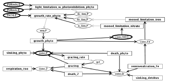
Figure 1: Graph of the process representation of the Ross Sea ecosystem model. Variables are represented as ovals and processes as rectangles. Arrows indicate direct causal influence between processes and entity variables. Light arrows indicate an algebraic relations, while dark arrows signify differential equation-based relationship. Observed and driving variables are highlighted with a bold outline.

Along with recovering the original model, the process modeling approach lets users explore alternative model structures with relative ease. Exhaustively searching the library, we would also find many subsets of the original model that may fit the observed data. Consider the alternative structure suggested by Tagliabue and Arrigo’s (2003) finding that zooplankton may not be a significant factor in the plankton dynamics of the Ross Sea. To explore this possibility, we could instantiate a model that excludes the zooplankton entity and its related processes. Within our framework, we would then compare the performance of this model to the original one to help determine which is most appropriate. If we wanted to expand the model so that it differentiates between P. antarctica and the diatom phytoplankton, we could simply instantiate the phytoplankton entity type twice (e.g., replace $P\{Phytoplankton\}$ in the entity declaration line with $phaeo\{Phytoplankton\}$ and $diatoms\{Phytoplankton\}$) and then instantiate the processes associated with phytoplankton a second time, assigning one set to each phytoplankton group. If the scientists do not believe the same processes impact the two groups, they can search through alternative process instantiations. Again, we can add new generic processes or alternative formulations of generic processes to the library and implement them with little difficulty. The ease with which users can develop and evaluate alternative model structures is one of the primary advantages of the process model formulation.

4 Related Research

The process modeling framework builds upon and relates to ideas already present in the literature. Here, we characterize the work’s relevance and novelty.

Modeling the processes that generate system dynamics is not a new idea in ecology. In their textbook, Jørgensen and Bendoricchio (2001) make a strong commitment to modeling specific processes. In Chapter 3, the authors describe several mathematical formulations of physical, chemical, and biological processes that commonly occur in ecological models. Gurney and Nisbet (1998) also discuss the importance of processes in modeling ecological dynamics, stating “formulation of a dynamic model always starts by identifying the fundamental processes in the system under investigation.” However, both texts switch to sets of equations after processes are considered during model formulation. An additional emphasis on processes in ecological modeling appears in the growing use of process-based models (e.g., Landsberg and Waring, 1997; Simioni et al., 2000; McMurtrie, 1985; Brugnach, 2005; Melillo et al., 1993; Reynolds and Ford, 1999; Galbraith et al., 1980). With an emphasis on processes, these models resemble those built with the approach described in this paper. Brugnach (2005) shows clearly that process-based models are conceptualized as a network of data flowing between processes that operate on the data. However, model actors or entities are not clearly delineated in this approach.

In an effort to create a general theory of modeling and simulation, Zeigler (1974) presents a framework that is very similar to the representation we describe. He describes models using three elements: components, descriptive variables, and component interactions. Components are the parts of the system from which the model is constructed. Variables (and parameters) characterize the properties of the individual components, and collectively portray the system’s behavior. Component interactions are the relationships linking components. From this description, it is seems that entities in our framework captures both Zeigler’s components and descriptive variables. Our processes are a subset of Zeigler’s component interactions. The difference between our representation and Zeigler’s approach stems from his desire to construct a general theory of modeling. In contrast, we focus on constructing continuous-time, simulation models of mechanisms.

Our conceptual framework is perhaps most similar to one described by Machamer et al. (2000) in their discussion of mechanisms in biology. They claim that mechanisms are composed of entities and activities. As in our framework, entities are the actors in a system, both creating and being affected by activities, which produce change in the system. Their activities seem equivalent to our processes, although the authors discuss and apply the framework to scientific reasoning in neurobiology and molecular biology. They do not show how it relates to the mathematical models that arise in ecology, and they do not develop their ideas into a clear working methodology.

As in the process modeling approach, some ecological research generates and tests alternative possibilities. At the broadest level, if we consider each candidate model structure as a hypothesis of the system’s structure and function or an alternative explanation for observed behavior, then searching the space of hypotheses is an extreme form of evaluating multiple alternative hypotheses (e.g., Loehle, 1987b; Carpenter et al., 1998; Hilborn and Mangel, 1997). More closely related is the work of Jost and Arditi (2001), who manually fit models with alternative formulations of the predation process to several predator–prey data sets. Their objective was to determine whether predation was best explained by predator density-dependent or -independent processes. Although they compared alternative processes, they view their modeling approach as a statistical fitting and selection of nonlinear models to population data, a methodology gaining prominence in population ecology (e.g., Jost and Arditi, 2000, 2001; Hilborn and Mangel, 1997; Carpenter et al., 1994). However, their approach lacks an explicit notion of modeling as search.

The most closely related research is the approach to model revision introduced by Reynolds and Ford (1999). They describe a multi-criteria assessment technique for evaluating process-based models that is used in an iterative modeling cycle to guide revision of both model structure and parameter selection. Like the modeling approach discussed in this paper, the goal is to discover better model formulations. Two important differences stem from the fact that their approach does not provide a way to specify domain theory a priori. First, their procedure only allows revision of an existing model; I t cannot guide search for the initial model. Second, the methodology detects and generally locates model deficiencies, but it cannot suggest specific model revisions to make. The scientist must manually revise the model and then reapply the multi-criteria assessment.

5 Directions for Future Work

As the Ross Sea model shows, the approach described in this paper can be an effective tool for constructing, organizing, and communicating complicated models. However, there remain several ways in which the approach can be advanced. In particular, we see three ways of extending our approach to improve its utility for modeling environmental phenomena.

The first extension involves implementing a hierarchical organization of both entities and processes. Part of the complexity of environmental systems is that their components operate and interact with each other at multiple scales of space and time. Hierarchical entities and processes are one way to capture this complexity that matches how biologist and ecologists tend to think about them (Ahl and Allen, 1996; Allen and Starr, 1982; O’Neill et al., 1986). For example, organisms are classified using a taxonomic hierarchy. The White-throated Sparrow (Zonotrichia albicollis) is in the family Emberizidae, which is in the class Aves of the Animal kingdom (National Geographic Society, 1999). Members of each taxonomic level share certain properties that are used to classify them. We may also use hierarchical entities to encode spatial phenomena. We envision using a set of entities to represent different physical locations, where each “spatial entity” contains relevant entities and processes for that space. For example, in a lake ecosystem model we might represent the areas above and below the thermocline as two distinct entities. Finally, hierarchical processes would let us explicitly represent exudation and nutrient uptake in the Ross Sea ecosystem model as subprocesses of growth. We have already begun work on developing ways to represent and use such hierarchical processes (Todorovski et al., 2005).

The second extension addresses the criteria for selecting models. Information about ecological systems is typically heterogeneous; ecologists generally know more about some parts of the system then others. For example, they may have continuous-time observations for some system variables but only know the appropriate ranges or general trajectory shapes for others. Scientists often evaluate the plausibility of simulation models using all of these criteria (e.g., Arrigo et al., 2003). At present, Prometheus only provides information about standard goodness-of-fit measures for the variables with continuous-time data. Although we may use this additional information to evaluate the models manually, we may also be able to encode the information and use it to guide automated search and selection of appropriate models.

Finally, this modeling methodology creates new possibilities for analyzing system behavior. Sensitivity analysis is commonly used in ecological modeling to determine the effect of varying one or more parameters on the model behavior. However, we expect that performing a process-level sensitivity analysis will lead to increased understanding of system dynamics because it will reveal which processes are primarily responsible for dynamics at a given time. This information will be useful for guiding additional experimental work, as well as assisting environmental assessment and management. Using the more common process-based ecological modeling approach, Brugnach (2005) provides an initial example of how such process sensitivity analysis might work.

6 Summary

In this paper, we described a novel method for representing and developing simulation models of complex ecological and environmental systems. The representation builds on a two-part ontology that includes entities and processes. With this formalism, we represent quantitative models in a way that approximates how scientists think about systems. We also develop reusable libraries of generic entities and processes based on existing ecological knowledge. We claim that these libraries link model development to existing theory, facilitate model evaluation, and expedite model construction.

Two features contribute to the novelty of our modeling approach. First, we view model construction as search through a space of possible models. Second, we instantiate model elements from generic components. The space of theoretically plausible models and the generic components are defined in libraries of domain specific entities and processes. We expect this approach to facilitate the construction of ecological models both for theoretical development and for environmental assessment and management.

7 Acknowledgements

This research was supported by NSF Grant No. IIS-0326059 and by NTT Communication Science Laboratories, Nippon Telegraph and Telephone Corporation.

References

- Abarca-Arenas and Ulanowicz (2002) Abarca-Arenas, L. G., Ulanowicz, R. E., 2002. The effects of taxonomic aggregation on network analysis. Ecological Modelling 149, 285–296.
- Abrams (1993) Abrams, P. A., 1993. Why predation rate should not be proportional to predator density. Ecology 74, 726–733.
- Abrams (2000) Abrams, P. A., 2000. The impact of habitat selection on the spatial heterogeneity of resources in varying environments. Ecology 81, 2902–2913.
- Ahl and Allen (1996) Ahl, V., Allen, T. F. H., 1996. Hierarchy Theory: A Vision, Vocabulary, and Epistemology. Columbia University Press, New York.
- Allen and Starr (1982) Allen, T. F. H., Starr, T. B., 1982. Hierarchy: Perspectives for Ecological Complexity. University of Chicago Press, Chicago.
- Arrigo and Tagliabue (2005) Arrigo, K. R., Tagliabue, A., 2005. Iron in the Ross Sea: 2. Impact of discrete iron addition strategies. Journal of Geophysical Research–Oceans 110, C03010.
- Arrigo et al. (2003) Arrigo, K. R., Worthen, D. L., Robinson, D. H., 2003. A coupled ocean–ecosystem model of the Ross Sea: 2. Iron regulation of phytoplankton taxonomic variability and primary production. Journal of Geophysical Research–Oceans 108, C73231.
- Asgharbeygi et al. (2006) Asgharbeygi, N., Bay, S., Langley, P., Arrigo, K., 2006. Inductive revision of quantitative process models. Ecological Modelling 194, 70–79.
- Beck (1987) Beck, M. B., 1987. Water-quality modeling: A review of the analysis of uncertainty. Water Resources Research 23, 1393–1442.
- Bossel (1992) Bossel, H., 1992. Real-structure process description as the basis of understanding ecosystems and their development. Ecological Modelling 63, 261–276.
- Brando et al. (2004) Brando, V. E., Ceccarelli, R., Libralato, S., Ravagnan, G., 2004. Assessment of environmental management effects in a shallow water basin using mass-balance models. Ecological Modelling 172, 213–232.
- Brugnach (2005) Brugnach, M., 2005. Process level sensitivity analysis for complex ecological models. Ecological Modelling 187, 99–120.
- Cale et al. (1989) Cale, W. G., Henebry, G. M., Yeakley, J. A., 1989. Inferring process from pattern in natural communities: Can we understand what we see? Bioscience 39, 600–605.
- Cale and Odell (1979) Cale, W. G., Odell, P. L., 1979. Concerning aggregation in ecosystem models. In: Halfon, E. (Ed.), Theoretical Systems Ecology. Academic Press, New York, pp. 55–77.
- Carpenter et al. (1998) Carpenter, S. R., Cole, J. T., Essington, T. E., Hodgson, J. R., Houser, J. N., Kitchell, J. F., Pace, M. L., 1998. Evaluating alternative explantations in ecosystem experiments. Ecosystems 1, 335–344.
- Carpenter et al. (1994) Carpenter, S. R., Cottingham, K. L., Stow, C. A., 1994. Fitting predator–prey models to time series with observation errors. Ecology 75, 1254–1264.
- Carpenter et al. (1985) Carpenter, S. R., Kitchell, J. F., Hodgson, J. R., 1985. Cascading trophic interactions and lake productivity: Fish predation and herbivory can regulate lake ecosystems. Bioscience 35, 634–639.
- Clark et al. (2001) Clark, J. S., Carpenter, S. R., Barber, M., Collins, S., Dobson, A., Foley, J. A., Lodge, D. M., Pascual, M., Pielke, R., Pizer, W., Pringle, C., Reid, W. V., Rose, K. A., Sala, O., Schlesinger, W. H., Wall, D. H., Wear, D., 2001. Ecological forecasts: An emerging imperative. Science 293, 657–660.
- Costanza and Ruth (1998) Costanza, R., Ruth, M., 1998. Using dynamic modeling to scope environmental problems and build consensus. Environmental Management 22, 183–195.
- Ford (2000) Ford, E. D., 2000. Scientific Method for Ecological Research. Cambridge University Press, Cambridge; New York.
- Galbraith et al. (1980) Galbraith, K. A., Arnold, G. W., Carbon, B. A., 1980. Dynamics of plant and animal production of a subterranean clover trifolium-subterraneum pasture grazed by sheep 2. Structure and validation of the pasture growth model. Agricultural Systems 6, 23–43.
- Gardner et al. (1982) Gardner, R. H., Cale, W. G., O’Neill, R. V., 1982. Robust analysis of aggregation error. Ecology 63, 1771–1779.
- George et al. (2003) George, D., Saito, K., Langley, P., Bay, S., Arrigo, K., 2003. Discovering ecosystem models from time-series data. Proceedings of the Sixth International Conference on Discovery Science, 141–152.
- Gold (1977) Gold, H. J., 1977. Mathematical Modeling of Biological Systems: An Introductory Guidebook. Wiley, New York.
- Grant et al. (1997) Grant, W. E., Pedersen, E. K., Marin, S. L., 1997. Ecology and Natural Resource Management: Systems Analysis and Simulation. John Wiley and Sons, Inc., New York.
- Gurney and Nisbet (1998) Gurney, W. S. C., Nisbet, R. M., 1998. Ecological Dynamics. Oxford University Press, New York.
- Hilborn and Mangel (1997) Hilborn, R., Mangel, M., 1997. The Ecological Detective: Confronting Models with Data. Princeton University Press, Princeton, N.J.
- Hornberger and Spear (1980) Hornberger, G. M., Spear, R. C., 1980. Eutrophication in Peel Inlet–1. The problem-defining behavior and a mathematical model for the phosphorus scenario. Water Research 14, 29–42.
- Jørgensen (1994) Jørgensen, S. E., 1994. Models as instruments for combination of ecological theory and environmental practice. Ecological Modelling 75-76, 5–20.
- Jørgensen (2002) Jørgensen, S. E., 2002. Integration of Ecosystem Theories: A Pattern, 3rd Ed. Kluwer Academic Publishers, Dordrecht.
- Jørgensen and Bendoricchio (2001) Jørgensen, S. E., Bendoricchio, G., 2001. Fundamentals of Ecological Modelling, 3rd Ed. Elsevier, New York.
- Jost and Arditi (2000) Jost, C., Arditi, R., 2000. Identifying predator–prey processes from time-series. Theoretical Population Biology 57, 325–337.
- Jost and Arditi (2001) Jost, C., Arditi, R., 2001. From pattern to process: Identifying predator–prey models from time-series data. Population Ecology 43, 229–243.
- Korfmacher (2001) Korfmacher, K. S., 2001. The politics of participation in watershed modeling. Environmental Management 27, 161–176.
- Landsberg and Waring (1997) Landsberg, J. J., Waring, R. H., 1997. A generalized model of forest productivity using simplified concepts of radiation-use efficiency carbon balance and partitioning. Forest Ecology Management 95, 209– 228.
- Langley (2000) Langley, P., 2000. The computational support of scientific discovery. International Journal of Human-Computer Studies 53, 393–410.
- Langley et al. (2003) Langley, P., George, D., Bay, S., Saito, K., 2003. Robust induction of process models from time-series data. Proceedings, Twentieth International Conference on Machine Learning 1, 432–439.
- Langley et al. (2002) Langley, P., Sánchez, J., Todorovski, L., Džeroski, S., 2002. Inducing process models from continuous data. Proceedings of the Nineteenth International Conference on Machine Learning, 347–354.
- Langley et al. (in press) Langley, P., Shiran, O., Shrager, J., Todorovski, L., Pohorille, A., in press. Constructing explanatory process models from biological data and knowledge. AI in Medicine.
- Langley et al. (1987) Langley, P., Simon, H. A., Bradshaw, G. L., Żytkow, J. M., 1987. Scientific Discovery: Computational Explorations of the Creative Processes. MIT Press, Cambridge, MA.
- Levins (1966) Levins, R., 1966. The strategy of model building in population biology. American Scientist 54, 421–431.
- Levins (1993) Levins, R., 1993. Formal analysis and the fluidity of science — a response. Quarterly Review of Biology 68, 547–555.
- Loehle (1987a) Loehle, C., 1987a. Errors of construction, evaluation, and inference: A classification of sources of error in ecological models. Ecological Modelling 36, 297–314.
- Loehle (1987b) Loehle, C., 1987b. Hypothesis testing in ecology: Psychological aspects and the importance of theory maturation. Quarterly Review of Biology 62, 397–409.
- Machamer et al. (2000) Machamer, P., Darden, L., Craver, C. F., 2000. Thinking about mechanisms. Philosophy of Science 67, 1–25.
- Maguire (2003) Maguire, L. A., 2003. Interplay of science and stakeholder values in Neuse River total maximum daily load process. Journal of Water Resources Planning and Management 129, 261–270.
- McMurtrie (1985) McMurtrie, R. E., 1985. Forest productivity in relation to carbon partitioning and nutrient cycling: A mathematical model. In: Cannell, M. G. R., Jackson, J. E. (Eds.), Attributes of Trees as Crop Plants. Institute of Terrestrial Ecology. Natural Environment Research Council, Abbots Ripton, Huntington, UK.
- Melillo et al. (1993) Melillo, J. M., McGuire, A. D., Kicklighter, D. W., Moore, B., Vorosmarty, C. J., Schloss, A. L., 1993. Global climate change and terrestrial net primary production. Nature 363, 234–239.
- National Geographic Society (1999) National Geographic Society, 1999. Field Guide to the Birds of North America, 3rd Ed. National Geographic, Washington, D.C.
- O’Neill et al. (1986) O’Neill, R. V., DeAngelis, D. L., Waide, J. B., Allen, T. F. H., 1986. A Hierarchical Concept of Ecosystems. Princeton University Press, Princeton, New Jersey.
- Oreskes (1998) Oreskes, N., 1998. Evaluation (not validation) of quantitative models. Environmental Health Perspectives 106, 1453–1460.
- Oreskes et al. (1994) Oreskes, N., Shraderfrechette, K., Belitz, K., 1994. Verification, validation, and confirmation of numerical-models in the earth-sciences. Science 263, 641–646.
- Orzack and Sober (1993) Orzack, S. H., Sober, E., 1993. A critical assessment of Levins’s the strategy of model-building in population biology (1966). Quarterly Review of Biology 68, 533–546.
- Osidele and Beck (2004) Osidele, O. O., Beck, M. B., 2004. Food web modelling for investigating ecosystem behaviour in large reservoirs of the south-eastern United States: Lessons from Lake Lanier, Georgia. Ecological Modelling 173, 129–158.
- Pulliam and Danielson (1991) Pulliam, H. R., Danielson, B. J., 1991. Sources, sinks, and habitat selection — a landscape perspective on population-dynamics. American Naturalist 137, S50–S66.
- Rastetter et al. (1992) Rastetter, E. B., King, A. W., Cosby, B. J., Hornberger, G. M., O’Neill, R. V., Hobbie, J. E., 1992. Aggregating fine-scale ecological knowledge to model coarser-scale attributes of ecosystems. Ecological Applications 2, 55–70.
- Reckhow (1994) Reckhow, K. H., 1994. Water quality simulation modeling and uncertainty analysis for risk assessment and decision making. Ecological Modelling 72, 1–20.
- Reynolds and Ford (1999) Reynolds, J. H., Ford, E. D., 1999. Multi-criteria assessment of ecological process models. Ecology 80, 538–553.
- Sage et al. (2003) Sage, R. W., Patten, B. C., Salmon, P. A., 2003. Institutionalized model-making and ecosystem-based management of exploited resource populations: A comparison with instrument flight. Ecological Modelling 170, 107–128.
- Saltelli et al. (2000) Saltelli, A., Chan, K., M., S. E. (Eds.), 2000. Sensitivity Analysis. John Wiley and Sons, Chichester, U.K.
- Sánchez and Langley (2003) Sánchez, J. N., Langley, P., 2003. An interactive environment for scientific model construction. Proceedings of the Second International Conference on Knowledge Capture, 138–145.
- Simioni et al. (2000) Simioni, G., Le Roux, X., Gignoux, J., Sinoquet, H., 2000. Treegrass: A 3-D, process-based model for simulating plant interactions in tree–grass ecosystems. Ecological Modelling 131, 47–63.
- Spear and Hornberger (1980) Spear, R. C., Hornberger, G. M., 1980. Eutrophication in Peel Inlet–2. Identification of critical uncertainties via generalized sensitivity analysis. Water Research 14, 43–49.
- Tagliabue and Arrigo (2003) Tagliabue, A., Arrigo, K. R., 2003. Anomalously low zooplankton abundance in the Ross Sea: An alternative explanation. Limnology and Oceanography 48, 686–699.
- Tagliabue and Arrigo (2005) Tagliabue, A., Arrigo, K. R., 2005. Iron in the Ross Sea: 1. Impact on CO2 fluxes via variation in phytoplankton functional group and non-Redfield stoichiometry. Journal of Geophysical Research–Oceans 110, C03009.
- Todorovski et al. (2005) Todorovski, L., Bridewell, W., Shiran, O., Langley, P., 2005. Inducing hierarchical process models in dynamic domains. Proceedings of the Twentieth National Conference on Artificial Intelligence, 892–897.
- Underwood (1997) Underwood, A. J., 1997. Experiments in Ecology: Their Logical Design and Interpretation Using Analysis of Variance. Cambridge University Press, Cambridge; New York.
- Whipple et al. (2005) Whipple, S. J., Patten, B. C., Verity, P. G., 2005. Life cycle of the marine alga Phaeocystis: A conceptual model to summarize literature and guide research. Journal of Marine Systems 57, 83–110.
- Worthen and Arrigo (2004) Worthen, D. L., Arrigo, K. R., 2004. A coupled ocean–ecosystem model of the Ross Sea. Part 1: Interannual variability of primary production and phytoplankton community structure. In: DiTullio, G. R., Dunbar, R. B. (Eds.), Biogeochemistry of the Ross Sea. Vol. 78 of Antarctic Research Series. American Geophysical Union, Washington, DC.
- Zeigler (1974) Zeigler, B. P., 1974. Theory of Modelling and Simulation, 2nd Ed. Robert E. Krieger Publishing Company, Malabar, Florida.