Episodic synchronization in dynamically driven neurons

Abstract

We examine the response of type II excitable neurons to trains of synaptic pulses, as a function of the pulse frequency and amplitude. We show that the resonant behavior characteristic of type II excitability, already described for harmonic inputs, is also present for pulsed inputs. With this in mind, we study the response of neurons to pulsed input trains whose frequency varies continuously in time, and observe that the receiving neuron synchronizes episodically to the input pulses, whenever the pulse frequency lies within the neuron’s locking range. We propose this behavior as a mechanism of rate-code detection in neuronal populations. The results are obtained both in numerical simulations of the Morris-Lecar model and in an electronic implementation of the FitzHugh-Nagumo system, evidencing the robustness of the phenomenon.

I Introduction

Neurons exhibit all-or-none responses to external input signals. The main function of this thresholding behavior is to process information in a way that is efficient and robust to noise lindner04 . Input signals received by most non-sensory neurons take the form of pulse trains, coming from the spiking activity of neighboring neurons. Therefore, in order to understand the mechanisms of information processing in neural systems, it is very important to characterize in detail the response of neurons to pulse trains. Furthermore, realistic pulse trains are intrinsically dynamical, with an instantaneous firing frequency that varies continuously in time. It is therefore necessary to assess the influence of this non-stationarity in the neuronal response. This paper addresses these questions.

Most studies of driven neurons have been restricted so far to harmonic driving signals lee99 ; yu01 ; parmananda02 ; laing03 ; sthilaire04 . Many of these works have shown that for certain types of neurons, i.e. those exhibiting what is called type II excitability, a resonant behavior arises with respect to the external driving frequency. Excitability in those neurons is usually associated with an Andronov-Hopf bifurcation, which leads to the existence of subthreshold oscillations in the excitable regime. When the frequency of these oscillations equals that of the harmonic driving, a resonance arises.

It is to be expected that a similar resonant behavior exists for pulsed inputs. In that case, the same pulse train impinging on two different neurons could elicit a response on only one of them, i.e. on the one that is tuned to resonate with the incoming pulse frequency. This behavior has indeed been observed experimentally in a rat’s neocortical pyramidal neuron that innervates another pyramidal neuron and an interneuron; a bursting input from the innervating neuron produced an action potential in the interneuron but not in the second pyramidal neuron markram98 . This behavior was interpreted in terms of a differential frequency-dependent facilitation and depression, respectively, and as such was studied by Izhikevich and co-workers izhikevich02 ; izhikevich03 . Here we propose a simpler mechanism for this phenomenon, relying only on the resonant behavior of the processing neuron. This mechanism could provide a means for distinguishing between firing rates, whose controlled variation lies at the heart of the rate coding approach to information processing by neurons.

Our results show that type II excitable neurons exhibit a resonant response with respect to the frequency of input pulse trains. This behavior leads to episodic synchronization between the neuron’s output and an input with dynamically varying firing rate. Episodic synchronization has previously been reported in coupled lasers with intrinsic dynamics buldu06 . Here we extend that property to externally driven excitable systems. Two types of systems have been investigated: a Morris-Lecar model (Sec. II) and an electronic implementation of the FitzHugh-Nagumo model (Sec. III).

II Morris-Lecar model

II.1 Model description

We consider neurons whose dynamical behavior is described by the Morris-Lecar model morris81 ,

$$\frac{dV}{dt} = \frac{1}{C_{m}}(I_{\rm app}-I_{\rm ion}-I_{\rm syn})+D\xi(t)$$ (1)

$$\frac{dW}{dt} = \phi\Lambda(V)[W_{\infty}(V)-W]$$ (2)

where $V$ and $W$ represent the membrane potential and the fraction of open potasium channels, respectively. $C_{m}$ is the membrane capacitance per unit area and $\phi$ is the decay rate of $W$. The neuron is affected by several currents, including an external current $I_{\rm app}$, a synaptic current $I_{\rm syn}$, and an ionic current given by

$$I_{\rm ion}=g_{Ca}M_{\infty}(V)(V-V^{0}_{Ca})+$$

$$\qquad\qquad\qquad g_{K}W(V-V^{0}_{K})+g_{L}(V-V^{0}_{L})\,.$$ (3)

In this expression, $g_{a}$ ($a=Ca,K,L$) are the conductances and $V^{0}_{a}$ the resting potentials of the calcium, potassium and leaking channels, respectively. We define the following functions of the membrane potential:

$$M_{\infty}(V)=\frac{1}{2}\left[1+\tanh\left(\frac{V-V_{M1}}{V_{M2}}\right)\right]$$ (4)

$$W_{\infty}(V)=\frac{1}{2}\left[1+\tanh\left(\frac{V-V_{W1}}{V_{W2}}\right)\right]$$ (5)

$$\Lambda(V)=\cosh\left(\frac{V-V_{W1}}{2V_{W2}}\right)\,,$$ (6)

where $V_{M1}$, $V_{M2}$, $V_{W1}$ and $V_{W2}$ are constants to be specified later. The last term in Eq. (1) is a white Gaussian noise term of zero mean and amplitude $D$.

In the absence of noise, an isolated Morris-Lecar neuron shows a bifurcation to a limit cycle for increasing applied current $I_{\rm app}$ sthilaire04 . Depending on the parameters, this bifurcation can be of the saddle-node or the subcritical Hopf types, corresponding to either type I or type II excitability, respectively. The specific values of the parameters used are shown in table 1 tsumoto06 . For these parameters, the threshold values of the applied current under constant stimulation are $39.7$ mA for type I and $46.8$ mA for type II.

In this paper we analyze the behavior of a neuron driven by a synaptic current. To that end, we use the simplified model of chemical synapse proposed in Ref. destexhe , according to which the synaptic current is given by

$$I_{\rm syn}=g_{\rm syn}r(t)(V-E_{s}),$$ (7)

where $g_{\rm syn}$ is the conductance of the synaptic channel, $r(t)$ represents the fraction of bound receptors, and $E_{s}$ is a parameter whose value determines the type of synapse: if $E_{s}$ is larger than the rest potential the synapse is excitatory, if smaller it is inhibitory; here we consider an excitatory synapse with $E_{s}=0$ mV. The fraction of bound receptors, $r(t)$, follows the equation

$$\frac{dr}{dt}=\alpha[T](1-r)-\beta r\,,$$ (8)

where $[T]=T_{max}\theta(T_{0}+\tau_{\rm syn}-t)\theta(t-T_{0})$ is the concentration of neurotransmitter released into the synaptic cleft by the presynaptic neuron, whose dynamics is also given by Eqs. (1)-(2) with no synaptic input. $\alpha$ and $\beta$ are rise and decay time constants, respectively, and $T_{0}$ is the time at which the presynaptic neuron fires, which happens whenever the presynaptic membrane potential exceeds a predetermined threshold value, in our case chosen to be $10$ mV. This thresholding mechanism lies at the origin of the nonlinear character of the synaptic coupling. The time during which the synaptic connection is active is roughly given by $\tau_{\rm syn}$. The values of the coupling parameters that we use destexhe are specified in Table 1. The equations were integrated using the Heun method nises , which is a second order Runge-Kutta algorithm for stochastic equations.

Parameter	Morris-Lecar TII (TI)
$C_{m}$	$5\,\mu\mathrm{F/cm}^{2}$
$g_{K}$	$8\,\mu\mathrm{S/cm}^{2}$
$g_{L}$	$2\,\mu\mathrm{S/cm}^{2}$
$g_{Ca}$	$4.0\,\mu\mathrm{S/cm}^{2}$
$V_{K}$	$-80\,\mathrm{mV}$
$V_{L}$	$-60\,\mathrm{mV}$
$V_{Ca}$	$120\,\mathrm{mV}$
$V_{M1}$	$-1.2\,\mathrm{mV}$
$V_{M2}$	$18\,\mathrm{mV}$
$V_{W1}$	$2\,\mathrm{mV}$ ($12\,\mathrm{mV}$)
$V_{W2}$	$17.4\,\mathrm{mV}$
$\phi$	$1/15\,\mathrm{s}^{-1}$

Parameter	Synapse
$\alpha$	$2.0\,\mathrm{ms}^{-1}\mathrm{mM}^{-1}$
$\beta$	$1.0\,\mathrm{ms}^{-1}$
$T_{max}$	$1.0\,\mathrm{mM}$
$g_{\rm syn}$	(specified in each case)
$\tau_{\rm syn}$	$1.5\,\mathrm{ms}$
$E_{s}$	$0\,\mathrm{mV}$

Table 1: Parameters values of the Morris-Lecar and synapse models used in this work.

II.2 Response diagram of a periodically driven driven neuron

First we analyze how a Morris-Lecar neuron responds to periodic inputs of varying frequencies. Specifically, we ask how large the signal needs to be in order to elicit spikes in the receiving neuron. It is also important to characterize the frequency of spiking in terms of frequency of the input. As mentioned in the introduction, this question has already been addressed, in the case of harmonic inputs, for different neuronal models, including the Morris-Lecar model chinosML . We will now compare these results with those obtained for a pulsed input. For the Morris-Lecar model, one can expect a completely different behavior between the type I and the type II cases, given that the bifurcation to a limit cycle is a saddle-node bifurcation in the former case and a Hopf bifurcation (with the well known eigenfrequency associated to the spiral fixed point) in the latter.

We first consider an isolated neuron without synaptic inputs ($I_{\rm syn}=0$), but subject to a harmonic modulation of the applied current $I_{\rm app}$ with the form,

$$I_{\rm app}=I_{0}+A\cos(2\pi f_{\rm in}t)\,.$$ (9)

In order to quantify the response of the neuron to this harmonic input, we plot in Fig. 1 (in color scale) the ratio between the output and the input frequencies, $f_{\rm out}/f_{\rm in}$, as a function of the amplitude $A$ and frequency $f_{\rm in}$ of the applied current (9). The figure compares the resulting response diagrams of type I and type II neurons. To obtain these plots, $A$ is varied for fixed $f$, while using as initial condition for a given $A$ the final state of the previous $A$ value. In the upper panels $A$ increases, thus showing the stability of the rest state, while in the lower panels $A$ decreases, this indicating the stability of the limit cycle. The figure shows that type II neurons have a region of bistability, where the fixed point and the limit cycle coexist. In contrast, for type I neurons the two plots are basically the same, indicating and absence of bistability.

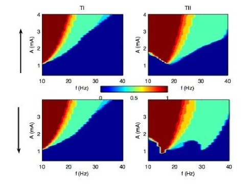
Figure 1: Response diagram of Morris Lecar neurons for a harmonic input: $f_{\rm out}/f_{\rm in}$ is plotted (color-coded) as a function of the amplitude and frequency of the applied current. Left plots: type I neuron (with $I_{0}=39$ mA), right plots: type II neuron (with $I_{0}=46$ mA). The response is measured for increasing $A$ in the upper plots, and for decreasing $A$ in the lower plots.

There is another qualitative difference between types I and II that can be observed in Fig. 1. In the type I neuron, the critical modulation amplitude for spiking increases monotonically with the frequency of the stimulus. On the other hand, in the type II neuron the critical amplitude exhibits a minimum for a given nonzero frequency, in our case around $20$ Hz. This behavior can be understood as resulting from the subthreshold damped oscillations characteristic of type II excitability sthilaire04 .

We now characterize the response of a neuron to an input train of periodic synaptic pulses of varying frequencies and amplitudes. To that end, we drive the neuron with a synaptic current with the form

$$I_{\rm syn}=A\,r(t,f_{\rm in})(V(t)-E_{s})\,.$$ (10)

In this model, the frequency is given by the dynamics of $r(t,f_{\rm in})$, described in Eq. (8), assuming that the presynaptic firings occur periodically with frequency $f_{\rm in}$. In this way, we can quantify the response of the neuron in terms of the efficiency in responding to a periodic synaptic input with a given frequency and amplitude, as shown in the harmonic case.

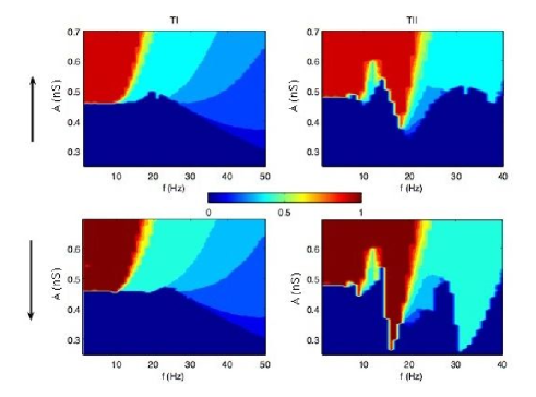
Figure 2: Response diagrams of Morris Lecar neurons to a periodic synaptic (pulsed) input: $f_{\rm out}/f_{\rm in}$ is plotted (in color scale) as a function of the amplitude and the frequency of the synaptic current. Left plots: type I neuron (with $I_{\rm app}=39$ mA), right plots: type II neuron (with $I_{\rm app}=46$ mA). The response is measured for increasing $A$ in the upper plots, and for decreasing $A$ in the lower plots.

Figure 2 shows the corresponding response diagrams, i.e. $f_{\rm out}/f_{\rm in}$ as a function of $A$ and $f_{\rm in}$, for both excitability types and for increasing (top) and decreasing (bottom) $A$. The behavior shows features common to the harmonic case, such as the existence of the same resonant frequency in type II for both kinds of inputs. But there are also very interesting differences between them, specially in the high and zero frequency limits.

The main difference between the harmonic and pulsed input cases is the approach to the DC threshold current ($39.7$ mA for type I and $46.8$ mA for type II). While in the former case this happens for frequencies approaching zero (type I) or resonance (type II), for pulsed inputs it happens for high frequencies, i.e. when the signal period is of the order of the pulse width. This is the reason for the appearance of a spiking region at high frequencies for pulsed inputs, which is absent in the harmonic case DC . Also, in the low-frequency limit one can observe, for pulsed inputs, a constant value of the critical amplitude. This is related with the fact that, when the input period is high enough with respect to the pulse width, the system response is essentially independent of the period.

II.3 The dynamical case: Variation of the input frequency

In the previous section, we have characterized the behavior of a neuron subject to a pulsed synaptic current of fixed frequency. Our results show that type II neurons exhibit a resonant behavior, defined by the existence of an optimal frequency for which the critical amplitude for spiking is minimal. The question now is, what happens if the frequency of the input train varies dynamically, which is a more realistic situation for a non-sensory neuron.

To answer this question, we made simulations with two Morris-Lecar neurons coupled unidirectionally through a chemical synapse. The input neuron operates in the limit cycle regime and is considered to be type I, so that we can control its spiking frequency by varying its applied current $I_{\rm app}$ sthilaire04 . This neuron is synaptically coupled to a type II neuron operating in an excitable regime, with a coupling strength $g_{\rm syn}$ such that the receiving neuron only fires in a given range of frequencies (i.e. the coupling is such that the amplitude of the input pulses lies below the critical amplitude at zero frequency but above its minimum at resonance; this corresponds e.g. to a horizontal line at around 0.4 mV in the right plots of Fig. 2).

Figure 3 shows what happens when the firing frequency of the input neuron first increases and then decreases in the range 13-28 Hz. The plot compares the instantaneous firing frequency of both neurons, relating them with the boundaries of the locking range of the second neuron, indicated by horizontal dashed lines; the 1:1 locking region is specifically shown.

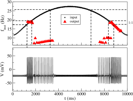
Figure 3: Upper plot: instantaneous frequency versus time of the input neuron (black stars) and of the receiving neuron (red triangles). The three horizontal dashed lines indicate the boundaries of the locking region for the selected synaptic strength ($g_{\rm syn}=0.43$ nS); the 1:1 region is specifically shown, and labeled at the right. Lower plot: time series of the receiving neuron.

It can be seen that as the input frequency increases (first half of the plot), the receiving neuron starts spiking with approximately 1:1 frequency ratio when the input frequency falls within the corresponding locking range, the ratio decreasing when the input frequency exceeds $\sim$20 Hz. Spiking persists while the input frequency remains in the wider (not 1:1) locking range, and is maintained even for a while after the input finally exits the locking region. A similar behavior is observed for decreasing frequencies, but the “inertia” observed at the exit of the locking region is larger than for increasing frequencies. The time series of the receiving neuron is shown in the lower plot; the episodes of synchronization with the input signal are clearly observed.

In order to understand the dynamic driving effects reported above, and particularly the locking asymmetry observed between an increase and a decrease in the input firing frequency, we now study the neuron response to a controlled variation of the frequency for different variation rates. To that end, we consider a synaptic input whose frequency is uniformly changing from one cycle to the next at a rate $f^{\prime}=\Delta f/\Delta t$, and measure the response of the neuron in terms of its instantaneous output frequency $f_{\rm out}$. Figure 4 shows the response diagram for a fixed synaptic strength and different frequency variation rates, for both increasing and decreasing input frequencies $f_{\rm in}$.

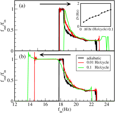
Figure 4: Response of a type II neuron to a controlled variation of the input frequency, for two different rates of this variation, $f^{\prime}=\Delta f/\Delta t$, for $g_{\rm syn}=0.38$ nS, compared with the adiabatic response (which is a horizontal cut of the response diagram at $A=0.38$ nS).

The figure shows that the slower the variation rate, the closer the response is to an adiabatic passage, as expected. Additionally, the results indicate that the persistence of the output neuron in the firing state (even when the input signal has left the locking region) is much larger when the frequency decreases than when it increases. This is consistent with the asymmetric response exhibited in Fig. 3, and can be expected to arise from the asymmetric shape of the response function $f_{\rm out}/f_{\rm in}$, which is equal to 1 for small frequencies and moderately smaller than 1 for large frequencies. Evidently the neuron prefers to respond in a 1:1 regime, which produces a larger persistence for decreasing frequencies.

To further quantify the approach to the adiabatic response in terms of the rate of change in the input frequency, we can define a distance ${\cal D}$ to this adiabatic response as the absolute value of the difference between the area of the neuron’s response diagram at a given rate $f^{\prime}$, as plotted in Fig. 4, and the area of the adiabatic response:

$${\cal D}=\int_{f_{\rm min}}^{f_{\rm max}}\left[\left(\frac{f_{\rm in}}{f_{\rm out}}\right)_{f^{\prime}}-\left(\frac{f_{\rm in}}{f_{\rm out}}\right)_{\rm adiab}\right]df_{\rm in}\,.$$ (11)

This measure is plotted in the inset of Fig. 4 as a function of the rate of change in the input frequency. The plot shows that the distance increases as the frequency changes more rapidly, as expected.

The dynamical response described in the previous paragraphs leads to episodic synchronization when the input pulse train exhibits a varying firing rate. This situation is shown in Fig. 5, in which an input pulse train whose firing rate takes the form, by way of example, of an Ornstein-Uhlenbeck noise with amplitude $A_{\rm ou}=0.1$ mA and correlation time $\tau_{\rm ou}=1$ s in the $\sim 20-36$ Hz range. The response of the second neuron for $g_{\rm syn}=0.38$ nS is displayed in the bottom plot, and exhibits clear episodes of synchronization with the input signal, whenever the firing rate of the later falls (approximately) within the locking range of the neuron for the coupling strength chosen (represented by horizontal dashed lines in the figure). In that way the receiving neuron acts as a bandpass filter for input pulse trains.

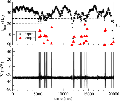
Figure 5: Upper panel: Instantaneous frequency of the synaptic input (black stars) and of the output neuron (red triangles) as a function of time. The horizontal dashed lines delimit the region of locking according to the adiabatic calculations of Fig. 2 for the synaptic strength used ($g_{\rm syn}=0.38$ nS). Lower panel: time series of the input signal.

III FitzHugh-Nagumo circuit

In order to show that the behavior reported in the previous Section is generic and robust, we have reproduced the results with an electronic neuron, specifically with an electronic implementation of the FitzHugh-Nagumo (FHN) model nagumo64 . The circuit has been previously described in tor03 , where synchronization between two FHN neurons was studied. A detailed description of the circuit can be found at circuit . In our particular setup, a FHN neuron is excited by a pulsed input of variable frequency.

Following the procedure of Sec. II, we first determine the response of the electronic neuron to a train of periodic pulsed inputs of fixed frequency. The pulses have the form of square pulses of $10$ ms width. Figure 6 shows the corresponding response diagram, obtained by increasing the amplitude of the input pulses until the neuron starts firing. Similar results (not shown here) are obtained with pulses of different width.

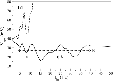
Figure 6: Response diagram of an electronic FHN neuron for a periodic input of pulses with $10$ ms width. The limit of the region of 1:1 resonance is marked with a dashed line.

At first glance, we can observe a resonance minimum around $f_{\rm in}=15$ Hz, which confirms that the FHN neuron is of type II. Two local minima are also observed around $f_{\rm in}=7.5$ Hz and $f_{\rm in}=31$ Hz. It is worth noting that despite the spike threshold is low, moderately large values of the input voltage are required to induce spiking at the input frequency (see region 1:1 in Fig. 6).

We have thus a type II electronic neuron that exhibits a resonance at a frequency close to $15$ Hz. Following again the approach of Sec. II, we now subject the circuit to pulse trains with time-varying frequency. Specifically, the pulse frequency is made to depend linearly with time (with both positive and negative slope). Similar results (not shown here) are obtained with sinusoidal variations. The neuron response to this dynamical input is shown in Figs. 7 and 8, where two different input voltages, corresponding to the values denoted as A and B in Fig. 6, have been applied.

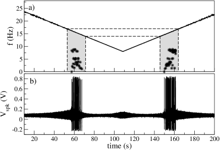
Figure 7: Response of a FHN electronic neuron to a pulsed input of variable frequency. The input voltage corresponds to the value marked by A in Fig. 6. Plot (a) shows the instantaneous frequency of the input pulses (solid line) and of the neuron’s output (stars). The shaded region corresponds to the frequency ranges for which locking should occur. Plot (b) displays the time evolution of the membrane voltage of the electronic neuron, which corresponds with the voltage U2 at condenser C1, in the circuit given in circuit .

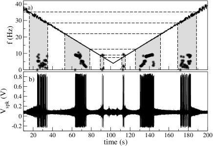
Figure 8: Response of a FHN electronic neuron to a pulsed input of variable frequency. The input voltage corresponds to the value marked by B in Fig. 6. Figure layout is as described in the caption of Fig. 7.

In the case of Fig. 7, the input signal scans the region marked with $A$ in Fig. 6. The upper plot shows the instantaneous frequency of the input train (solid line) and of the FHN neuron (stars). Figure 7(b) plots the neuron’s output. The results show that the neuron pulses when the input frequency lies within the resonance regions given in Fig. 6, and highlighted in gray in Fig. 7(a). This behavior is an agreement with the observations made in the Morris-Lecar model. The fact that no inertia effects are seen when the input frequency sweeps past the resonance region is due to the frequency variation rate being very slow with respect to the characteristic time scales of the system (adiabatic limit).

Figure 8 shows the system’s behavior for a different value of the input voltage (marked as B in Fig. 6), for which the input frequency encounters three resonance regions as it varies. Accordingly, the electronic neuron fires whenever the input frequency lies inside any these regions, exhibiting clear episodes of synchronization. In other words, the neuron acts as a band-pass filter, with a frequency range that depends on the input voltage level according to its response diagram.

IV Discussion

Neurons are information-processing devices. The nature of coding in neuronal systems is still an open question. One of the most favored views in the field is that of rate coding, where the intensity of a signal is encoded in the firing rate. Neuronal systems must therefore be able to distinguish between firing rates. We have proposed a way to accomplish that, through the resonant behavior exhibited by type II neurons. A population of neurons with different tuning characteristics, and therefore distinct locking ranges, should be able to distinguish between different incoming pulse frequencies by activating selectively different subpopulations that respond selectively to different frequencies.

We have systematically analyzed the response of type I and II neurons to pulsed driving, compared it with the standard case of sinusoidal driving, and observed the resonant behavior of type II neurons. This phenomenology leads to episodic synchronization between the input and the output of the neuron, when the input consists of a train of pulses with dynamically varying frequency. The phenomenon has been reported both in numerical simulations of the Morris-Lecar model, and in an experimental implementation of the FitzHugh-Nagumo circuit. We expect this type of behavior to underlie information processing in rate coding and decoding neuronal populations in more complex brain networks.

- (1) B. Lindner, J. García-Ojalvo, A. Neiman, and L. Schimansky-Geier, Phys. Rep. 392, 321 (2004).
- (2) S.-G. Lee and S. Kim, Phys. Rev. E 60, 826 (1999).
- (3) Y. Yu, F. Liu, and W. Wang, Biol. Cybern. 84, 227 (2001).
- (4) P. Parmananda, C.H. Mena, and G. Baier, Phys. Rev. E 66, 047202 (2002).
- (5) C.R. Laing and A. Longtin, Phys. Rev. E 67, 051928 (2003).
- (6) M. St-Hilaire and A. Longtin, J. Comp. Neurosc., 16, 299-313, (2004).
- (7) H. Markram, Y. Wang, and M. Tsodiks, Proc. Natl. Acad. Sci. USA 95, 5323 (1998).
- (8) E.M. Izhikevich, Biosystems 67, 95 (2002).
- (9) E.M. Izhikevich, N.S. Desai, E.C. Walcott, and F.C. Hoppensteadt, Trends Neurosci. 26, 161 (2003).
- (10) J.M. Buldú, T. Heil, I. Fischer, M.C. Torrent, and J. Garcia-Ojalvo. Phys. Rev. Lett. 96, 024102 (2006).
- (11) C. Morris and H. Lecar, Biophys. J. 35, 193 (1981).
- (12) K. Tsumoto, H. Kitajima, T. Yoshinaga, K. Ahiara, and H. Kawakami, Neurocomp. 69, 293 (2006).
- (13) A. Destexhe, Z. F. Mainen, and T. J. Sejnowski, Neural Comp. 6, 14 (1994).
- (14) J. García-Ojalvo and J. M. Sancho, Noise in Spatially Extended Systems (Springer, New York, 1999).
- (15) J. Xie, J.-X. Xu, Y.-M. Kang, S.-J. Hu, and Y.-B. Duan, Chin. Phys. 13, vol. 9, 1396 (2004).
- (16) In top left panel of Fig. 2, the spiking region stretches down below nS, a lower value than expected. This happens because the amplitude of the synaptic pulses is larger than , due to modulation by the term shown in Eq. (10).
- (17) J. Nagumo, S. Arimoto, and S. Yoshizawa, Proc. IRE 50, 2061 (1964).
- (18) R. Toral, C. Masoller, C.R. Mirasso, M. Ciszak and O. Calvo, Physica A 325, 192 (2003).
- (19) http://www-fen.upc.es/donll/info/FHNcircuit.pdf.