Dynamics of Semiflexible Polymers in a Flow Field

Abstract

We present a novel method to investigate the dynamics of a single semiflexible polymer, subject to anisotropic friction in a viscous fluid. In contrast to previous approaches, we do not rely on a discrete bead-rod model, but introduce a suitable normal mode decomposition of a continuous space curve. By means of a perturbation expansion for stiff filaments we derive a closed set of coupled Langevin equations in mode space for the nonlinear dynamics in two dimensions, taking into account exactly the local constraint of inextensibility. The stochastic differential equations obtained this way are solved numerically, with parameters adjusted to describe the motion of actin filaments. As an example, we show results for the tumbling motion in shear flow.

I Introduction

In the course of evolution, nature found a both amazingly simple and robust way to sustain the mechanical stability of biological cells, while at the same time providing them with extraordinary dynamic capabilities, like growing, moving, and dividing. The basic structure elements making this possible are semiflexible polymers, in the cytoskeleton present in form of F-actin, intermediate filaments and microtubuli. Two characteristic properties distinguish them from most of the other natural and synthetic polymers: They possess a certain stiffness which energetically suppresses bending, and they are to a high degree inextensible, i.e., their backbone cannot be stretched or compressed. Moreover, electric charge and polarity effects as well as the ability to assemble and disassemble are essential for the dynamics of the whole cytoskeleton network.

In the last 15 years enormous progress has been made in experimental observation and theoretical description of these physical aspects. To give some examples, fluorescence video microscopy of labeled filaments has allowed for the detailed study of statistic properties of F-actin Käs et al. (1996), DNA Maier and Rädler (1999), and microtubules Pampaloni et al. (2006). Quantities like the end-to-end distance Wilhelm and Frey (1996) and force-extension relations Kroy and Frey (1995) have been calculated and verified experimentally Bustamante et al. (2003); Le Goff et al. (2002a), the latter being accessible by means of optical and magnetical tweezers. Furthermore, fluorescence correlation spectroscopy Lumma et al. (2003); Winkler et al. (2006); Shusterman et al. (2004) and light scattering Kroy and Frey (1997) have been used to obtain, e.g., the mean square displacement and dynamic structure factor.

In this paper we concentrate on the theoretical description of the dynamics of a single semiflexible polymer. This is the relevant model not only in the dilute limit, but also essential for the understanding of the medium and high frequency response of networks of semiflexible filaments Gardel et al. (2004). Concerning the theory, the textbook models of Rouse and Zimm Doi and Edwards (1986) have to be extended, since they apply to Gaussian chains only and thus fail to incorporate the effects of semiflexibility. A systematic analysis of the dynamics was limited in this field to the linear regime until recently, when the dynamic propagation and relaxation of tension could be elucidated Bohbot-Raviv et al. (2004); Hallatschek et al. (2004), and a comprehensive, unified theory worked out Hallatschek et al. (2005). The numerical approach usually adopted for polymeric systems is to construct a polymer from a finite number of beads, each of which is connected with two neighbors by a stiff rod or spring Bird et al. (1987). Our goal is to set up a different method more suited to the subtleties of semiflexibility, such that the numerical description of these filaments becomes tractable when they are subjected to fluid flow. The purpose of this work is twofold: First, we want to establish a new method that covers the above-mentioned goals, and second, the results we present in applying this technique are directly relevant to experiments with polymers in a shear flow.

Many authors have addressed systems with semiflexible polymers by means of different bead–rod/spring based techniques Ermak and McCammon (1978); Fixman (1978); Grassia and Hinch (1996); Morse (2004); Hofmann et al. (2000). However, maintaining the mechanical constraint of a constant bond length becomes complicated with increasing resolution, since it couples the motion of all beads. The controversial question arises whether this requirement has to be implemented as a literally rigid constraint or by an infinitely stiff potential, since these two cases differ in their statistical mechanics van Kampen and Lodder (1984). One often chooses to address an infinitely stiff bead-spring chain by means of a rigidly constrained system, which is more feasible concerning computational time. Then, an additional pseudo-potential has to be applied to guarantee the correct equilibrium Boltzmann distribution Hinch (1993); Pasquali and Morse (2002). Moreover, timescales present major limitations when solving stiff systems numerically Everaers et al. (1999). The characteristic relaxation time of a bending mode imposed on the filament is inversely proportional to the fourth power of the corresponding wavenumber. The largest wavenumber that can be resolved by discretized models is proportional to the number of beads. Hence the time step one has to choose is inversely proportional to the quartic number of monomers, for the shortest wavelength undulations to be sampled correctly. At the same time, the longest mode needs to have enough time to relax to equilibrium, and since these two times differ by the fourth power of the resolution of the spatial discretization, the necessary computational time can become prohibitively long.

As a consequence, the numerical approach has been limited, when semiflexible systems with constraints were to be investigated. Some dynamic properties could be grasped by a suitable combination of multiple short runs Everaers et al. (1999), but this is not possible when further external timescales enter, which do not match the intrinsic limitations. For instance, this is the case when the polymer is subject to a fluid flow. Corresponding simulations have been reported with a quite small resolution of nine beads Montesi et al. (2005). On the other hand, experiments of this type have already been carried out for DNA Perkins et al. (1997); Smith et al. (1999); Teixeira et al. (2005); Schroeder et al. (2005a); Gerashchenko and Steinberg (2006), and simulations have been presented to examine their findings Hur and Shaqfeh (2000); Schroeder et al. (2005b); Puliafito and Turitsyn (2005). Indeed, the latter have always been done with models that allow for a finite or even infinite extensibility of the chains. This might be a suitable approach for coil–like DNA molecules, but it would miss important physics, if applied to stiffer filaments like F-actin or (pre–)stretched DNA Obermayer et al. (2006).

Recently, a new idea has been presented Wiggins et al. (2003) for an alternative approach that avoids these difficulties for two-dimensional systems. This concept starts from a continuous model for the semiflexible polymer and uses a suitable normal mode analysis. Some of these ideas have been utilized before to describe the deterministic Becker and Shelley (2001), linear behaviour of semiflexible filaments in a viscous solution Wiggins (1998). However, the extension to the nonlinear case at finite temperature has proven to be subtle, and it is the goal of this work to consistently establish the approach and explore some of the possibilities it can offer.

II Method

In our model, a semiflexible polymer is represented by a space curve $\vec{r}(s,t)$, parameterised by the arclength $s$ (Fig. 1). The minimal model for the description of a semiflexible polymer in this representation is the wormlike chain Kratky and Porod (1949); Saitô et al. (1967), valid when the detailed properties on the atomic and monomeric scale are not important anymore Doi and Edwards (1986). Then, the hamiltonian for the elastic energy is given by the integral of the squared curvature $c(s,t)$, multiplied with the bending modulus $\kappa$,

$$\mathcal{H}_{\text{el}}=\frac{\kappa}{2}\int_{0}^{L}\!ds\,c^{2}.$$ (1)

The bending modulus can be expressed in terms of the persistence length $\ell_{p}$, the characteristic length for the exponential decay of the tangent autocorrelation (Landau and Lifschitz, 1987, §127):

$$\kappa=k_{B}T\ell_{p}(\mathrm{dim}-1)/2,$$ (2)

where “dim” denotes the dimension of the embedding space. For synthetic polymers, the persistence length is typically of the order of the polymer’s diameter, $\ell_{p}\approx a$. The tangential correlations thus decay very fast, hence these polymers are called flexible. Semiflexible are polymers with $\ell_{p}\gg a$, which is the case for the biopolymers inside the cell. Depending on the ratio of contour length and persistence length we can distinguish different regimes: In case of DNA one usually deals with the flexible limit, $L\gg\ell_{p}$; in this work however we are exploring the stiff regime, where $\ell_{p}\geq L$. The latter matches in nature, e.g., to the properties of F-actin and microtubuli.

Figure 1: Sketch of a polymer of length $L$, represented by a continuous space curve $\vec{r}(s,t)$. An example is shown for the local unit tangent vector $\hat{t}(s,t)$, as well as the end-to-end distance vector $\vec{R}$.

Due to low Reynolds numbers, the motion of $\mu$m-sized objects like biopolymers in solution is overdamped, i.e., friction exceeds inertia by several orders of magnitude Frey and Kroy (2005). As a consequence, inertia terms can safely be neglected, and the equations of motion are of first order in time. The stochastic dynamics of a polymer in a quiescent solvent can thus be described by the Langevin equation Doi and Edwards (1986); Kroy and Frey (2000)

$$\frac{\partial}{\partial t}\vec{r}(s,t)=\int_{0}^{L}\!ds^{\prime}\,\mathbf{H}[\Delta\vec{r}\,]\left\{-\frac{\delta\mathcal{H}[\vec{r}(s^{\prime\prime},t)]}{\delta\vec{r}(s^{\prime},t)}+\vec{\xi}(s^{\prime},t)\right\}.$$ (3)

Here $\mathbf{H}[\Delta\vec{r}\,]$ is the mobility tensor, with $\Delta\vec{r}\,\equiv\vec{r}(s,t)-\vec{r}(s^{\prime},t)$, and $\vec{\xi}$ the noise, which we assume to be Gaussian distributed with mean zero. The energetic part of the Hamiltonian $\mathcal{H}[\vec{r}\,]$ is given by $\mathcal{H}_{\text{el}}$, and we will discuss necessary additions below.

Concerning hydrodynamics, we adopt the free draining approximation, i.e., neglect all nonlocal interactions. This approximation can be justified by evaluating the Fourier transformation of the Green’s function of a hydrodynamic force field (Oseen tensor), which gives only a very weak, i.e. logarithmic, mode dependence of the mobility Frey and Nelson (1991). The underlying physical rationale is the mostly straight conformation of a stiff filament. For the same reason, excluded volume effects can safely be neglected. We implement the local friction of the polymer by using the anisotropic mobility of a stiff rod, which differs by a factor of two for the motion parallel and perpendicular to its tangent vector $\hat{t}=\partial_{s}\vec{r}$. Hence $\mathbf{H}[\Delta\vec{r}\,]\to\boldsymbol{\mathcal{P}}(r(s,t))\delta(s-s^{\prime})$, with the local mobility Doi and Edwards (1986); Batchelor (1970)

$$\boldsymbol{\mathcal{P}}=\mu_{\perp}\hat{n}\otimes\hat{n}+\mu_{\parallel}\,\hat{t}\otimes\hat{t}\,.$$ (4)

Here, $\hat{n}$ denotes the unit normal vector. The tangent and normal vector are related by the Frenet-Serret-equations, which in two dimensions read $\partial_{s}{\hat{t}}=c\hat{n}$, $\partial_{s}{\hat{n}}=-c\hat{t}$. The friction coefficients (per length) are obtained from the solvent viscosity $\eta$ and polymer diameter $a$ by $\mu_{\perp}=\frac{1}{2}\mu_{\parallel}=\ln(L/a)/2\pi\eta$.

Due to the presumed Gaussian nature of the noise we only need to specify the second moment of $\vec{\xi}$. By relating Eq. (3) to the appropriate Smoluchowski equation Gardiner (2004) and requiring a Boltzmann distribution in equilibrium we obtain

$$\langle\vec{\xi}(s,t)\otimes\vec{\xi}(s^{\prime},t^{\prime})\rangle=2k_{B}T\boldsymbol{\mathcal{P}}^{-1}\delta(s-s^{\prime})\delta(t-t^{\prime}).$$ (5)

Based on physical considerations given in appendix A we will interpret the noise according to Ito van Kampen (2001). In fact, some of the algebra necessary in the following relies on this interpretation.

A further important ingredient to the wormlike chain model is the inextensibility of the filament: We assume the local length to be constant by imposing the constraint $\partial_{s}\vec{r}\,^{2}\equiv\hat{t}\,^{2}=1$. To satisfy it, we introduce a Lagrange multiplier function $\Lambda(s,t)$ such that the full Hamiltonian reads Goldstein and Langer (1995)

$$\mathcal{H}=\mathcal{H}_{\text{el}}-\frac{1}{2}\int_{0}^{L}\!ds\,\Lambda(s,t)[\partial_{s}\vec{r}(s,t)]^{2}.$$ (6)

Although the constraint is identically satisfied in the arclength parameterization, we do need a Lagrange multiplier function here to make the variation of the coordinates in Eq. (3) independent of each other . In the following, we will be able to solve the equations of motion perturbatively for the Lagrange multiplier $\Lambda(s,t)$, hence the validity of the inextensibility constraint is guaranteed locally for all times. Physically, $\Lambda(s,t)$ corresponds to the tension acting against forces that would elongate or compress the filament’s backbone.

In evaluating the functional derivative of Eq. (6) we obtain from Eq. (3) the nonlinear equation of motion

$$\dot{\vec{r}}-\boldsymbol{\Gamma}\cdot\vec{r}=\boldsymbol{\mathcal{P}}\left\{-\kappa\vec{r}\,^{\prime\prime\prime\prime}-{(\Lambda\vec{r}\,^{\prime})}^{\prime}+\vec{\xi}\right\}.$$ (7)

On the left hand side we have subtracted the incompressible, homogeneous flow $\vec{u}=\boldsymbol{\Gamma}\cdot\vec{r}$ to account for the influence of an externally driven flow field. In Eq. (7) and the following, a prime indicates a derivative with respect to the arclength.

When constrained systems similar to Eq. (7) are approximated by discrete bead–rod models, one has to introduce a pseudo-potential (also called metric force) for the system to evolve into the correct equilibrium state Fixman (1978); Hinch (1993); Montesi et al. (2005). In contrast, we use a spectral approach, in which the arclength dependence is continuous (before explicitly evaluated on a computer, of course), but we truncate the expansion in terms of a finite number of wavelengths. Evaluating the metric determinant by means of the recursion relation proposed in Ref. Fixman (1974) leads to contributions proportional to powers of the spatial resolution. Thus in case of a continuous representation, we do not need to bother corrections of this kind.

To grasp the essential physics we will from now on consider the two-dimensional motion of a filament in a three-dimensional embedding fluid. This is actually a standard situation for experiments Maier and Rädler (1999); Teixeira et al. (2005), since the interesting dynamics is often restricted to two dimensions, while still allowing for a three-dimensional transfer of momentum to the environment. Note that this is distinct from systems where the hydrodynamics is confined to two dimensions. Thus in the following, the analysis will be presented for $\text{dim}=2$, cf. Eq. (2). The tangent and normal vectors then are given by (Fig. 1) $\hat{t}=(\cos\theta,\sin\theta)$, and $\hat{n}=(-\sin\theta,\cos\theta)$. To transform the equation of motion to variables which are scalar, we differentiate Eq. (7) with respect to the arclength and project the result onto the normal and tangent vector, respectively. Using the Frenet-Serret-Equations, we arrive at

$$\begin{split}\dot{\theta}&=\hat{n}\cdot\boldsymbol{\Gamma}\cdot\hat{t}+\mu_{\perp}\left\{-\kappa\left[c^{\prime\prime\prime}-(d+1)\left(c^{3}\right)^{\prime}\right]\right.\\ &\hskip 25.83325pt\left.-(d+1)\Lambda^{\prime}c-\Lambda c^{\prime}+\left[\hat{n}\partial_{s}+(d-1)c\hat{t}\right]\cdot\vec{\xi}\right\},\end{split}$$ (8)

$$\begin{split}0&=\hat{t}\cdot\boldsymbol{\Gamma}\cdot\hat{t}+\mu_{\perp}\left\{-\kappa\left[c^{4}-3d(cc^{\prime})^{\prime}-cc^{\prime\prime}\right]\right.\\ &\hskip 43.05542pt\left.+c^{2}\Lambda-d\Lambda^{\prime\prime}+\left[d\,\hat{t}\partial_{s}+(d-1)c\hat{n}\right]\cdot\vec{\xi}\right\}.\end{split}$$ (9)

These equations describe the motion of a semiflexible filament in its center of mass inertia frame, since the information on the absolute coordinate gets lost in evaluating the additional derivative of Eq. (7). The constant $d$ gives the ratio of parallel and perpendicular friction, $\mu_{\perp}=\mu_{\parallel}/d$. Slender-body hydrodynamics is described by the anisotropic case ($d=2$), physically corresponding to the difference in drag between normal and tangential motion of a slender body in Stokes flow. The simpler isotropic equations are obtained with $d=1$.

II.1 Normal Mode Analysis

The leading contribution governing the elastic dynamics of Eq. (8) is the second term on the right hand side, $-\kappa\partial_{s}^{3}c(s,t)=-\kappa\partial_{s}^{4}\theta(s,t)$. For a suitable normal mode decomposition of the equations (8) and (9) we thus may use the eigenfunctions of the biharmonic operator $\partial_{s}^{4}$. In this paper, we consider free boundary conditions $\vec{r}\,^{\prime\prime}(0)=\vec{r}\,^{\prime\prime}(L)=0$, $\vec{r}\,^{\prime\prime\prime}(0)=\vec{r}\,^{\prime\prime\prime}(L)=0$ Landau and Lifschitz (1991); Wiggins et al. (1998), corresponding to the situation of a filament fluctuating freely in flow. In angular coordinates this translate into

$$\theta^{\prime}(0)=\theta^{\prime}(L)=0\text{, and }\theta^{\prime\prime}(0)=\theta^{\prime\prime}(L)=0.$$ (10)

Furthermore, the tension has to vanish at the boundaries, $\Lambda(0)=\Lambda(L)=0$.

The biharmonic operator is not Hermitian with respect to a single set of eigenfunctions obeying (10); however, it is Hermitian with respect to a biorthogonal set of functions, where the first set $w^{\alpha}(s)$ obeys the boundary conditions of Eqs. (10), and the second set $w_{\alpha}(s)$ satisfies

$$w_{\alpha}(0)=w_{\alpha}(L)=0\text{, and }w_{\alpha}^{\prime\prime\prime}(0)=w_{\alpha}^{\prime\prime\prime}(L)=0.$$ (11)

These functions are solutions of the eigenvalue problems $\partial_{s}^{4}w^{\alpha}={k_{\alpha}^{4}}/{L^{4}}\,w^{\alpha}$, $\partial_{s}^{4}w_{\alpha}={k_{\alpha}^{4}}/{L^{4}}\,w_{\alpha}$, respectively, with identical eigenvalues $k_{\alpha}^{4}$, to be found from the solvability condition $\cos k_{\alpha}\cosh k_{\alpha}=1$. The general solutions $w^{\alpha}(s)$, $w_{\alpha}(s)$ are linear combinations of trigonometric and hyperbolic functions Landau and Lifschitz (1991), and a polynomial of third order for the zeroth eigenvalue $k_{0}=0$. They are explicitly given in App. B. Some nice experimental snapshots of the mode dynamics of F-actin can be found in Ref. Vonna et al. (2005).

The completeness of these two sets of eigenfunctions has not been shown yet. Neither a variational approach Courant and Hilbert (1967) nor a comparison with a complete basis Brauer (1965) seem to work in our case. However, we do not regard this as a major issue, since the failure is only due to our specific nonstandard set of boundary conditions—for other boundary conditions completeness can be shown Courant and Hilbert (1967). Furthermore, in order to implement the spectral approach, we will have to truncate all mode expansions, anyway.

We make use of the two sets of eigenfunctions to obtain normal mode expansions of the angle and tension (latin indices always start from 1, greek ones from 0):

$$\theta(s,t) =\theta_{0}(t)+\epsilon\sum_{j=1}^{\infty}\theta_{j}(t)w^{j}(s),$$ (12)

$$\Lambda(s,t) =\sum_{\nu=0}^{\infty}\Lambda^{\nu}(t)w_{\nu}(s).$$ (13)

In the first line we have separately written the zeroth mode $\theta_{0}(t)$, since it is independent of the arclength; it describes the motion of a stiff rod. The higher modes include undulations with successively smaller wavelength. The perturbation parameter $\epsilon$ will be defined by equipartition, as illustrated below. Equivalently, the zeroth tension mode $\Lambda^{0}(t)$ gives the tension distribution in a straight rod. By using the spectral expansion of the tension in the second line we assigned two additional boundary conditions to the tension [rightmost part of Eq. (11)]. We do not expect this vanishing cubic contribution to be a noticeable restriction to the tension at the edges. However, there is no simple physical interpretation to it.

As a first application of the mode expansions we insert Eq. (12) into the wormlike chain Hamiltonian (1), which in two dimensions can be written as

$$\mathcal{H}_{\text{el}}=\frac{\kappa}{2}\int_{0}^{L}\!ds\,(\partial_{s}\theta)^{2}.$$

By means of the equipartition theorem and Eq. (2) we get an expression for the mean size of the mode amplitudes (cf. App. B), dependent only on the relative persistence length:

$$\epsilon\sqrt{\langle\theta_{j}^{2}\rangle}=\sqrt{2\frac{L}{\ell_{p}}}\frac{1}{k_{j}}\,.$$ (14)

This suggests to define a flexibility parameter $\epsilon=\sqrt{L/\ell_{p}}$, which is small for stiff filaments. In the following section we will use $\epsilon$ to set up a perturbation expansion for the equations of motion. By definition Eq. (12), all angular modes $\theta_{\beta}$ are of order 1 with respect to this expansion.

II.2 Perturbation Expansion

The temperature $T$ enters the equation of motion in two ways: First, in the amplitude of the noise, Eq. (5), and second, in the expression for the bending stiffness, Eq. (2). A perturbation theory with respect to a single independent parameter $\epsilon$ will thus in general lead to different results, depending on the choice of the dependent parameter, $\kappa$ or $T$. However, a difference only appears in the expressions of cubic order in $\epsilon$. Since we aim to a solution in second order, this is of no concern for us. For concreteness, we choose the example of a constant curvature. Then, $\epsilon$ enters the equations only via the temperature in the noise correlator. We make all variables dimensionless by $t/B\to t$, $B=L^{4}/\kappa\mu_{\perp}$, $\vec{\xi}L^{3}/\epsilon\kappa\to\vec{\xi}$, $\Lambda L^{2}/\kappa\to\Lambda$, $\mu_{\perp}\boldsymbol{\mathcal{P}}^{-1}\to\boldsymbol{\mathcal{P}}^{-1}$, insert the expansions (12), (13) into the equations of motion and project them on mode $w_{\beta}$. The projection, if not evaluated, is abbreviated by

$$[\ldots]_{\beta}=\int_{0}^{L}\!ds\,w_{\beta}\ldots.$$

We furthermore introduce for the flow dependent terms

$$\dot{\gamma}g_{\beta}^{\parallel}=[\hat{t}\cdot\boldsymbol{\Gamma}\cdot\hat{t}\,]_{\beta}/L,\qquad\dot{\gamma}g_{\beta}^{\perp}=[\hat{n}\cdot\boldsymbol{\Gamma}\cdot\hat{t}\,]_{\beta}/L,$$

where $\dot{\gamma}$ is the strength of the flow in units of inverse seconds. $g_{\beta}$ are dimensionless, $\theta$-dependent functions that have to be expanded to the appropriate order. In these terms we obtain the following equations of motion:

$$\begin{split}\epsilon\,\partial_{t}\theta_{j}&=-\epsilon k_{j}^{4}\theta_{j}-\epsilon\!\!\sum_{\nu=0,i=1}\!\!\!\Lambda^{\nu}\theta_{i}\Xi^{i}_{j\nu}+\epsilon\eta_{j}^{\perp}\\ &\phantom{=}\,\,+B\dot{\gamma}g_{j}^{\perp}+\mathcal{O}(\epsilon^{3}),\end{split}$$ (15a)

$$\partial_{t}\theta_{0} =-\epsilon\!\!\sum_{\nu=0,i=1}\!\!\!\Lambda^{\nu}\theta_{i}\Xi^{i}_{0\nu}+\epsilon\eta_{0}^{\perp}+B\dot{\gamma}g_{0}^{\perp}+\mathcal{O}(\epsilon^{3}),$$ (15b)

$$0 =d\tilde{k}_{\beta}^{2}\Lambda^{\beta}+\epsilon\eta_{\beta}^{\parallel}+B\dot{\gamma}g_{\beta}^{\parallel}+\mathcal{O}(\epsilon^{2}).$$ (15c)

Here, a threefold overlap integral of eigenfunctions is abbreviated by

$$\Xi^{\alpha}_{\beta\nu}=\frac{1}{2}\left[(d+1)\int_{0}^{L}\!ds\,w^{\alpha}\left(\tilde{k}_{\nu}^{2}w^{\nu}w_{\beta}-\tilde{k}_{\beta}^{2}w^{\beta}w_{\nu}\right)\right.\\ \left.+(d-1)k_{\alpha}^{2}\int_{0}^{L}\!ds\,w_{\alpha}w_{\beta}w_{\nu}\right],$$ (16)

and the projected noise is expressed as

$$\begin{split}\eta_{\beta}^{\perp}&=\left[\left(\hat{n}\partial_{s}+(d-1)(\partial_{s}\theta)\hat{t}\,\right)\cdot\vec{\xi}\,\right]_{\beta},\\ \eta_{\beta}^{\parallel}&=\left[\left(d\,\hat{t}\partial_{s}+(d-1)(\partial_{s}\theta)\hat{n}\right)\cdot\vec{\xi}\,\right]_{\beta}.\end{split}$$ (17)

Note its dependence on $\epsilon$, via $\theta$ and via the unit vectors $\hat{t}$, $\hat{n}$. Furthermore we would like to mention that $g_{j}^{\perp}$ has no contribution to zeroth order in $\epsilon$, thus all terms of Eq. (15a) are at least linear in $\epsilon$. A linear stability analysis of the bending modes described by Eq. (15a) is obtained by expanding $g_{j}^{\perp}$ Wiggins et al. (2003). Finally, the dimensionless noise has the second moment

$$\langle\vec{\xi}(s,t)\otimes\vec{\xi}(s^{\prime},t^{\prime})\rangle=4\boldsymbol{\mathcal{P}}^{-1}\delta(s-s^{\prime})\delta(t-t^{\prime}).$$

Since the tension contribution to Eqs. (15a) and (15b) is always of first order in $\epsilon$, it is sufficient to expand it to one order less than the angular equations. For this reason Eq. (15c) is an algebraic equation. To obtain the given expression we have furthermore taken advantage of the eigenfunction’s property $w_{\alpha}^{\prime\prime}=-{\tilde{k}_{\alpha}^{2}}w^{\alpha}$ (see App. B). The tension modes $\Lambda^{\beta}$ can thus be inserted directly into the angular equations.

Concerning the noise, one obvious method to simplify Eqs. (17) would be to evaluate the projection integrals and find an expression for the correlation of the integrated noise. However, there are some complications in our case. It turns out that the correlation of the integrated noise is neither diagonal with respect to the mode projection (subscript $\beta$) nor with respect to the direction of the vector projection (superscripts $\perp$, $\parallel$). Furthermore, the order of the nondiagonal corrections is such that they have to be accounted for in an expansion up to order $\epsilon^{2}$. Thus a computational solution would have to include a numerical diagonalization of the conformation dependent noise in each step. To avoid this we diagonalize the inverse mobility matrix $\boldsymbol{\mathcal{P}}^{-1}$ analytically and calculate the arclength integrals in each time step by numerical means. As a drawback this includes the necessity of a fast random number generator, but still the implementation seems to us to be easier and faster.

The eigensystem of $\boldsymbol{\mathcal{P}}^{-1}=\hat{n}\otimes\hat{n}+\hat{t}\otimes\hat{t}/d$ can immediately be read off, and the corresponding transformation matrix $\mathbf{S}$ is used to rotate the noise locally, $\vec{\tilde{\xi}}:=\mathbf{S}\cdot\vec{\xi}$. For the calculation of the second moment of the rotated noise we necessarily need it to be of Ito type, since the matrix $\mathbf{S}$ is nonanticipating only in this case. We obtain

$$\left\langle\vec{\tilde{\xi}}(t,s)\otimes\vec{\tilde{\xi}}(t,s)\right\rangle=4\boldsymbol{\mathcal{P}}_{D}^{-1}\delta(t-t^{\prime})\delta(s-s^{\prime}),$$ (18)

where the diagonalized mobility matrix

$$\boldsymbol{\mathcal{P}}_{D}^{-1}=\mathbf{S}\cdot\boldsymbol{\mathcal{P}}^{-1}\cdot\mathbf{S}=\begin{pmatrix}1&0\\ 0&1/d\end{pmatrix}.$$

The new stochastic variable $\vec{\tilde{\xi}}$ simplifies the stochastic integrals (17) of the equations of motion:

$$\eta_{\beta}^{\perp} =\int_{0}^{1}\!ds\left(d\,{w}_{\beta}(\partial_{s}\theta)\tilde{\xi}_{2}-{w}_{\beta}^{\prime}\tilde{\xi}_{1}\right),$$ (19)

$$\eta_{\beta}^{\parallel} =-d\int_{0}^{1}\!ds\,{w}_{\beta}^{\prime}\tilde{\xi}_{2}+\mathcal{O}(\epsilon).$$ (20)

Using this in Eqs. (15) allows us to conveniently solve the coupled stochastic differential equations by numerical integration Kloeden and Platen (1995). The final equations without flow are a coupled set of linear equations (although of quadratic order in $\epsilon$) with multiplicative noise. Nevertheless, they cannot be solved analytically, due to the complicated structure of the coefficients.

III Results

III.1 Verification Without Flow Field

Figure 2: Mean squared amplitudes of normal modes for different persistence length. Open circles are numerical results, “+” interconnected by lines are given by Eq. (14). Significant deviations between both are visible only for $\epsilon=\sqrt{L/\ell_{p}}=1$. They are of order $\epsilon^{3}$, terms neglected in the perturbative solution Eq. (15a) (cf. also Fig. 3).

We have computed equilibrium averages of the squared mode amplitudes to compare them with the equipartition result, Eq. (14). This is to check the validity of the approximations we made in the previous section and of the numerical solution technique. For the first eleven modes shown in Fig. 2, the agreement is excellent in case of $\ell_{p}/L\geq 9$, i.e. $\epsilon\leq 1/3$. Slight deviations due to the limited validity of the $\epsilon$-expansion become visible at $\epsilon=1/3$; in case of $\epsilon=1$, results differ by about 14%. To analyze these errors in more detail, we have plotted the relative differences of analytical and numerical values for the mean square mode amplitudes versus $\epsilon^{-1}$ in Fig. 3. These relative errors decrease like $\epsilon^{2}$, as shown by the grey bar. This is consistent with our second order perturbation expansion, since the first terms we neglected are of third order, thus their contribution to the relative error is proportional to $\epsilon^{2}$.

In addition to that, Fig. 3 shows the relative errors of the mean end-to-end distance $R$ of the polymer. The corresponding exact result is $\langle R^{2}\rangle=L^{2}f_{D}(L/\ell_{p})$, with $f_{D}(x)=2(e^{-x}-1+x)/x^{2}$ Kratky and Porod (1949); Saitô et al. (1967). The deviations again decrease as expected proportional to $\epsilon^{2}$.

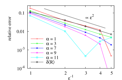
Figure 3: (Color online) Relative errors of some mean square mode amplitudes $\epsilon\sqrt{\langle\theta_{\alpha}^{2}\rangle}$ (colored) and mean end-to-end distance (black circles) versus inverse expansion parameter $\epsilon$. Lines are shown to guide the eye. As expected from the order of the expansion of the equations of motion, the relative error vanishes proportional to $\epsilon^{-2}$, thus the absolute error is $\propto\epsilon^{-3}$.

To validate dynamic properties, we compare the scaling behaviour of fluctuations of the mean square end-to-end distance (MSD) $\Delta_{R}(t)=\langle[R(t)-R(0)]^{2}\rangle$ with the analytically known and experimentally verified Granek (1997); Le Goff et al. (2002a) behaviour: For short times, $\Delta_{R}(t)$ grows subdiffusively like $t^{3/4}$, for long times it approaches the equilibrium value of $\Delta_{R}(t\to\infty)=2(L/\ell_{p})^{2}/45$. Our numerical results in Fig. 4 reproduce this pattern in excellent quality; effects of the perturbation expansion can only be seen in slight deviations from the expected plateau value at long times. Comparing Fig. 4 to corresponding experimental results (Fig. 3 of Ref. Le Goff et al. (2002a)) even shows a similar downturn for times $t/\tau_{1}<10^{-3}$. In case of Ref. Le Goff et al. (2002a) this is due to insufficient statistics at small times because of a limited observation period. In our case, the finite number of modes accounted for causes a slight suppression of fluctuations at these short times.

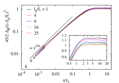
Figure 4: (Color online) Time dependence of the mean square displacement $\Delta_{R}(t)$ of the end-to-end distance. The calculations are done in 12-dimensional mode space. Symbols are replaced by lines were they would become very dense. The rescaled data for different persistence length collapses onto one master curve, which behaves $\propto t^{3/4}$ for short times. $\tau_{1}$ is the relaxation time of the longest mode, $\tau_{1}=k_{1}^{-4}$, in our units (cf. Eq. (15a), and Ref. Le Goff et al. (2002a)). The inset shows a magnification of the long-time behaviour. The stiffer the filament, the closer the numerical results are to the correct equilibrium value 1.

To summarize this part, we find that our method reproduces all tested equilibrium and dynamic observables very well within the accuracy expected from the perturbation expansion. In principle, one could think of even enhancing the accuracy of the equations. However, in spite of the simplicity of the equipartition expression, such a correction by means of an additional drift term is quite involved. This is caused by the strongly coupled nature of the equations, coming from the Lagrangian constraint and the noise projection. We dismissed such additions for this work, since the deviations are of minor importance for the applications we have in mind.

In the following section we will turn to an example of a nonequilibrium system that can nicely be worked out by means of the technique presented above. We always present results for filaments with persistence length $\ell_{p}/L\geq 4$, thus the systems show the correct equilibrium behaviour, as demonstrated by now.

III.2 Motion in Shear Flow

A shear flow is a laminar flow with a velocity field as depicted in Fig. 5. In terms of the velocity gradient matrix $\boldsymbol{\Gamma}$ this reads $\boldsymbol{\Gamma}=\dot{\gamma}\big{(}\begin{smallmatrix}0&1\\ 0&0\end{smallmatrix}\big{)}$, with respect to the coordinate axes of Fig. 1.

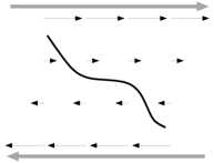
Figure 5: Sketch of a filament in shear flow. The two grey arrows indicate walls moving with constant speed, black arrows the velocity of the fluid. At the fluid–wall interface, the fluid is transported with the velocity of the wall, due to no-slip boundary conditions.

To gain some understanding of the basics we briefly discuss the case of a stiff rod exposed to shear. By re-implementing dimensionalized quantities in Eq. (15b) and afterwards taking the limit $\epsilon\to 0$ we obtain the equation of motion (cf. Ref. Puliafito and Turitsyn (2005))

$$\partial_{t}\theta_{0}(t)=-\dot{\gamma}\sin^{2}\theta_{0}(t)+\sqrt{D}\eta(t).$$ (21)

Here, the noise is $\delta$-correlated in time, and the diffusion constant $D=2\mu_{r}k_{B}T/L$, with the rotational mobility of a rod $\mu_{r}=\mu_{\perp}12/L^{2}$ Doi and Edwards (1986). In the deterministic case, i.e. $\eta\equiv 0$, Eq. (21) can be solved easily and results in a single rotation of the rod, which reaches the stall line at $\theta=0$ for long times like $t^{-1}$. In terms of stability analysis the deterministic dynamics corresponds to a flow on a circle with a half stable fixed point at $\theta=0$. When noise is present, $\eta$ is the control parameter of a saddle node bifurcation at $\eta=0$ Strogatz (2000). The effect of this is that the stochastic forces drive the rod across the stall line after some time, such that a new rotational cycle begins. Driven by the shear and the noise, the rod will now rotate again and again, such that one can e.g. measure the rotational times to characterize the stochastic process.

For finite $\epsilon$, we have the additional influence of the bending modes. Apart from shear-induced bending this can also change the behaviour close to the stagnation line, since filaments with curved conformations might wiggle easier across this threshold.

In Fig. 6 we show a sample trajectory of a filament with relative stiffness $\ell_{p}/L=6.5$. Here the rotations appear as a flip of the angular mode $\theta_{0}$ from $-\pi/2$ to $+\pi/2$. These flips are usually accompanied by a peak in the first mode $\theta_{1}$, indicating a sudden bending event triggered by the rotation. Furthermore, the end-to-end distance often shows a short dip corresponding to this intermediate bending.

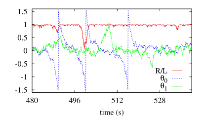
Figure 6: (Color online) Sample trajectories of the end-to-end distance $R$ and the first two angular modes, for a flow of strength $\dot{\gamma}=1.03$/s

Extensive experimental Smith et al. (1999); Schroeder et al. (2005a); Teixeira et al. (2005); Gerashchenko and Steinberg (2006), numerical Hur and Shaqfeh (2000); Montesi et al. (2005); Schroeder et al. (2005b); Puliafito and Turitsyn (2005), and some theoretical work Chertkov et al. (2005); Puliafito and Turitsyn (2005) has been presented to characterize the motion of DNA in shear flow. However, the relative persistence length $\epsilon^{-2}$ of DNA is typically about two to three orders of magnitude smaller than that of F-actin, as already denoted in the beginning of Sec. II. Consequently, the physics of these two kinds of semiflexible polymers will be quite different. When rotating in shear, for example, DNA more or less crawls along itself Schroeder et al. (2005a), whereas F-actin shows a clear stretch-out in our computations even at intermediate conformations, i.e., when the end-to-end distance is oriented perpendicular to the flow direction. Due to the different physics, the numerical methods used for DNA in the references above are not applicable in case of stiffer filaments like F-actin. In contrast to those techniques, our method always guarantees the local inextensibility of the filament.

A useful observable to get insight into the periodic and stochastic behaviour is the power spectral density (PSD) $P(f)$, the Fourier transformation of the autocorrelation function of an observable $x$:

$$P(f):=\mathcal{FT}\{\langle x(t)x(0)\rangle\}.$$

In Fig. 7 we show the PSD of the end-to-end distance $R$ of a filament with persistence length $\ell_{p}/L=6.5$, both with shear and without. The strength of the flow is $\dot{\gamma}=1.03/$s or $\mathrm{Wi}=0.55$, where $\mathrm{Wi}=\dot{\gamma}\tau_{c}$ is the dimensionless Weissenberg number, the product of flow rate and characteristic relaxation time $\tau_{c}$ of the system. For $\tau_{c}$ one may choose the mean exponential decay rate of the autocorrelation function of the end-to-end distance. In terms of the dimensionless formulation chosen in Sec. II.2, the bending stiffness $\kappa$ is constant, and only temperature varies when changing the stiffness parameter $\epsilon$. Thus in this formulation the relaxation rate is identical for all $\ell_{p}$. Our data result in a mean of $\tau_{c}=0.53\pm 0.02$ s, so flow rates $\dot{\gamma}$ have to be multiplied by this factor to obtain them in Wi-units.

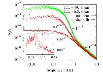
Figure 7: (Color online) Power spectral densities $P(f)$ of the end-to-end distance without flow, and with a shear of strength $\dot{\gamma}=1.03$ ($\mathrm{Wi}=0.55$). Green ‘x’: $\ell_{p}/L=49$, red ‘+’: $\ell_{p}/L=6.5$. The smooth black curve is a fit of the result in quiescent solvent with the appropriate Lorentzian Gittes and MacKintosh (1998), used for the plot of the relative PSD in Fig. 9. With shear, a bump between 0.05 and 0.09 Hz shows the characteristic time of rotation of the filament. A different scaling regime appears for frequencies smaller than 1 Hz, with an exponent depending on properties of the filament. PSD-data for $\ell_{p}/L=49$ have been multiplied by a factor 60 for the purpose of an easier visualization. Calculated with 10 ($\ell_{p}/L=6.5)$ and 8 ($\ell_{p}/L=49$) modes resolution. Inset: Nonlogarithmic version of the region around the bump for $\ell_{p}/L=6.5$, with estimated error bars. The number of data points has been reduced by averaging.

Without shear, the PSD shows a characteristic Lorentz-like behaviour, where the only timescale in the system separates the long time plateau from the short time decay. In case of the end-to-end distance $R$, the short time regime obeys the power law $P(f)\propto f^{-7/4}$ Gittes and MacKintosh (1998), which immediately follows from the mean square displacement $\propto t^{3/4}$. With shear, there is first of all a pronounced increase in correlations at small frequencies, indicating stronger long-time correlations due to periodic tumbling events. A shallow bump appears in the region between 0.05 and 0.09 Hz, indicating a typical frequency of rotation for the given flow strength. This bump is visible more clearly in Fig. 9, where we show the ratio of the PSDs with and without flow.

Coming back to Fig. 7, we identify an additional timescale in the decay for frequencies below 1 Hz, separating the high frequency power law $f^{-7/4}$ from a regime with an exponent with a larger absolute value. This intermediate sharp decay arises due to a subtle interplay between thermal fluctuations and frictional driving of the shear flow Hur and Shaqfeh (2000); Schroeder et al. (2005b). However, the power law of this decay is not generic—it depends on $\ell_{p}$ in a nontrivial manner. The detailed study of this phenomenon is deferred to a later publication.

In the experiments with DNA cited above, the end-to-end distance itself could not be measured due to the limited optical resolution; instead, the molecular extension was recorded, as measured by the mean projected extension in flow direction. However, it is reported that this observable does not show a typical frequency for a deterministic cycle associated with the tumbling motion in flow, in contrast to our results for the end-to-end distance of F-actin. We conjecture that this relatively weak effect might also be connected to the inextensibility of the filament.

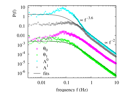
Figure 8: (Color online) Power spectral density of tension modes $\Lambda^{0}$, $\Lambda^{1}$, and angular modes $\theta_{0}$, $\theta_{1}$. Symbols give results with a shear flow of strength $\dot{\gamma}=1.03/s$ ($\mathrm{Wi}=0.55$). The light line (green online) shows the behaviour of $\theta_{1}$ without flow, smooth black curves are fitted Lorentzians, as explained in the text. A peak in $\theta_{0}$ and $\Lambda^{0}$ around 0.5 Hz is a sign of the tumbling time of the filament. Concerning $\theta_{1}$, shear still increases correlations at low frequencies.

Fig. 8 shows PSDs of the first two modes for the angle and tension. In the absence of flow, the stiff filament mode $\theta_{0}$ is to first order given by the rotational diffusion of a stiff rod. This leads to a $f^{-2}$ decay in the PSD with nonperiodic boundary conditions (not shown), which still gives the high frequency regime of the results in shear. The bumps of the PSDs of $R$ and $\theta_{0}$ are located at about the same frequency—in this regard it is interesting to note that the end-to-end distance is independent of $\theta_{0}$.

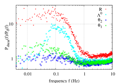
Figure 9: (Color online) Ratio of power spectral density $P(f)$ with shear flow to that without flow, for the data of Figs. 7 and 8. Correlations of $R$ are increased by a factor of more than 10 at frequencies of 0.3 Hz and below, with a peak between 0.05 and 0.09 Hz. Similarly, correlations of the first angular mode $\theta_{1}$ are pronounced by a factor of 2 below 0.1 Hz, and slightly decreased around 1 Hz. This is a signature of the semiflexible nature of the polymers under investigation, since it refers to the buckling events occurring periodically during their rotation in shear. Concerning the second angular mode $\theta_{2}$ (not shown in Fig. 8), there is still a change from decreased to increased correlations visible when going from $f=1$ Hz to 0.1 Hz and below. The tension mode $\Lambda^{0}$ shows a strong tenfold peak at 0.1 Hz when compared to a Lorentzian which has been fitted to the generic short- and long-time behaviour.

In a quiescent solvent, Eqs. (15) give Ornstein-Uhlenbeck behaviour for the higher angular modes $\theta_{i}$, with small deviations due to the coupling of the equations and the multiplicative noise. In Fig. 8 we only show the first mode $\theta_{1}$, where the case without flow has been fitted to a Lorentzian, whose coefficients differ from the Ornstein-Uhlenbeck process by at most some percent. The differences between observables recorded with and without flow are better visible in Fig. 9, where we identify an increase below 0.3 Hz and a slight decrease for higher frequencies. The increase of the plateau for $\theta_{1}$ is a characteristic of filaments with a relative persistence length of the order one: Stiffer filaments do not buckle at all during a rotation, and floppier ones show a different behaviour for strong flows (crawling near the stall line), or thermally fluctuate so heavily that a buckling due to shear cannot be identified. The next mode $\theta_{2}$ still shows a similar behaviour, but in an already much weaker manner.

The tension modes finally only show noise fluctuations around zero when no flow is present (not shown), which is obvious from Eq. (15c). In shear flow the power spectrum changes towards a behaviour as characteristic to Lorentzian curves for low and high frequencies. This is caused by the fact that there is a strong linear coupling between each tension mode $\Lambda^{\beta}$ and its corresponding angular mode $\theta_{\beta}$, visible by expanding the flow dependent part of Eq. (15c). The intermediate frequency region of the PSDs of the tension modes clearly shows signs of driving by shear: A bump, indicating a typical correlation time, followed by a sharp decay. These properties are even more pronounced in the tension modes, when comparing to the angular mode with the same index, respectively. In case of $\Lambda^{0}$ we identify a strong peak at the very same position of maximum height already mentioned for the PSDs of $\theta_{0}$ and $R$, and a sharper power law decay $f^{-3.6}$ towards higher frequencies. We conclude from this that the periodicity of the tumbling events can be found directly in the autocorrelation of the tension modes. This is very reasonable, since it follows that a rotation in shear triggers specific frictional forces acting on the backbone of the polymer, which have to be withstand by the constraining forces. In Fig. 9 we show the PSD of $\Lambda^{0}$ relative to a Lorentzian fitted to the generic short- and long-time behaviour to demonstrate the flow specific peak.

III.3 Statistics of Tumbling in Shear

A further point of interest is the mean time it takes the polymer to rotate. Experiments with DNA report a power law increase of the tumbling frequency with shear strength proportional to $\mathrm{Wi}^{0.67}$, confirmed by appropriate simulations and scaling analysis Schroeder et al. (2005a). Furthermore, analytic results for Brownian rods in strong shear consistently give $\mathrm{Wi}^{2/3}$ Puliafito and Turitsyn (2005).

Fig. 10 shows our results for the mean rotating frequency of filaments with various persistence lengths. We defined a flip to be a single half turn of an angle $\pi$. As a check of consistency, the frequency of rotation of a filament corresponding to Figs. 7 and 8 is $0.066\pm 0.002$ Hz, which lies very well within the observed peak width of these figures.

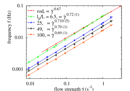
Figure 10: (Color online) Tumbling frequency of semiflexible polymers with different persistence length versus strength of shear flow. The change of the power law form $\dot{\gamma}^{0.72}$ at $\ell_{p}/L=6.5$ towards $\dot{\gamma}^{2/3}$ for a stiff rod indicates a crossover behaviour between rods and flexible polymers. The amplitude shift appears due to the parameterization we have chosen (cf. Sec. II.2) and has not been removed for reasons of readability.

The maximum flow strength for which we can obtain results numerically is limited by the $\epsilon$-expansion we have exploited in Sec. II.2. Since this expansion requires a small curvature, it breaks down when a powerful flow strongly bends the filament. For comparison we also plotted numerical results for a rotating stiff rod, which obeys the expected $\dot{\gamma}^{2/3}$ power law. The exponent shows a slight crossover behaviour in the semiflexible regime, in deviation from both the stiff and the flexible limit: As an example, the rotational frequency of a filament with persistence length $\ell_{p}/L=6.5$ scales like $\dot{\gamma}^{0.72\pm 0.01}$. The data of Fig. 10 furthermore demonstrate that the exponent becomes closer to 2/3 the stiffer the filament, as expected from the stiff rod limit. Note that this relatively weak crossover effect does not vanish $\propto\epsilon^{3}$, and thus seems not to be caused by deviations due to the perturbation expansion.

IV Conclusion

We have presented a newly developed method for describing the dynamics of single semiflexible filaments in a viscous solution, subject to external flow fields. Due to the mainly elongated conformations, hydrodynamic backflow effects are marginal and thus the dynamics can be formulated in the free draining approximation. In contrast to previous approaches based on bead-rod/spring models in real space we have adopted a spectral method of the equations of motion. A further simplification can be achieved upon using an angular representation of the polymer conformations. This has the advantage that there is no approximation in the bending energy. All of the above allows us to give an efficient computational approach for calculating Brownian trajectories for the polymers, and to include nonlinear effects of the environment without inherent limitations.

The computational time necessary for these numerical solutions is proportional to the fourth power of the mode number, and linear in the spatial resolution of the noise along the space curve. The main advantages regarding numerics are, compared to bead–rod models, first, mode dynamics offers a natural approach to the long-time dynamics, since the high wavenumber fluctuations are increasingly irrelevant (cf. Fig. 2). Second, the additional time necessary to satisfy the local constraint of constant length is very small. One reason for this is that no pseudo–potentials have to be calculated. Finally, one could even enhance the speed by adapting time and spatial resolution appropriately to each individual mode, a technique we did not apply, yet. In summary, we are able to monitor conformational properties very precisely, while taking account to all modes that give essential contributions to the dynamics of stiff semiflexible filaments.

Conceptually, our approach should be understood as being complementary to bead-rod and bead-spring models. In some cases the latter are advantageous, e.g. when dealing with dense solutions of flexible polymers, such that excluded volume effects are important.

Quantitative tests of the numerical solution show that the method correctly describes the fluctuations of semiflexible filaments in a quiescent solvent. We have demonstrated that our technique is capable of describing the long time dynamics in a sheared environment within reasonable computational time. For the first time we have calculated power spectral densities and mean rotational frequencies of F-actin in shear, taking into account exactly the local inextensibility constraint. The results have enabled us to point on two crossover phenomena still to be described in more detail. For the future, extensions of the method should be possible to include e.g. charge effects or different boundary conditions. A more challenging task is to extend the analysis to 3D.

An experimental test of the behaviour of Actin filaments in shear or elongational flow has not been reported, to our knowledge. However, the setup used for sheared DNA Smith et al. (1999); Schroeder et al. (2005a) might also work for F-actin, and elongational flows are constructed easily by means of microfluidic techniques Köster et al. (2005). Thus experiments could in principle be possible without too much technical effort.

Appendix A The Stochastic Integration

Stochastic equations are of Stratonovich type when the white noise they imply constitutes an approximation to a noise with finite correlation time. This seems to apply to us, since physically realistic random forces are never completely uncorrelated. However, this is not the only criterion for the decision, we also have to grasp correctly the physical relationship between the stochastic variable $\vec{r}$ and the noise $\vec{\xi}$ present in our specific system van Kampen (2001). The term we have to decide about is the mobility $\boldsymbol{\mathcal{P}}$, since it multiplies the noise in Eq. (7). Its physical meaning is to separate locally the velocity of the filament into a component parallel to its local tangent and another perpendicular to it. This separation will always refer to the current conformation and velocity of the space curve at that very moment of time; it will be unaffected by any stochastic forces in the future. This amounts to the definition of a nonanticipating function Gardiner (2004), and is equivalent to the demand to interpret the noise according to Ito.

Appendix B Eigenfunctions

The normalized biharmonic eigenfunctions obeying the boundary conditions of Eqs. (10) and (11) are

$$w^{0} =1\,,$$ (22)

$$\begin{split}w^{i}&=\frac{\cos k_{i}-\cosh k_{i}}{\sin k_{i}-\sinh k_{i}}\left(\cos\frac{k_{i}}{L}s+\cosh\frac{k_{i}}{L}s\right)\\ &\phantom{=}\;+\sin\frac{k_{i}}{L}s-\sinh\frac{k_{i}}{L}s\>,\end{split}$$ (23)

$$w_{0} =6\frac{s}{L}\left(1-\frac{s}{L}\right)\,,$$ (24)

$$\begin{split}w_{i}&=\frac{\cos k_{i}-\cosh k_{i}}{\sin k_{i}-\sinh k_{i}}\left(\cos\frac{k_{i}}{L}s-\cosh\frac{k_{i}}{L}s\right)\\ &\phantom{=}\;+\sin\frac{k_{i}}{L}s+\sinh\frac{k_{i}}{L}s\,.\end{split}$$ (25)

They are biorthonormal,

$$\int_{0}^{L}\!ds\,w^{\alpha}w_{\beta}=L\delta^{\alpha}_{\beta}.$$ (26)

A useful property of these eigenfunctions is

$${w^{\alpha}}^{\prime\prime}=-{k_{\alpha}^{2}}/{L^{2}}\,w_{\alpha},\qquad w_{\alpha}^{\prime\prime}=-{\tilde{k}_{\alpha}^{2}}/{L^{2}}\,w^{\alpha}.$$

Here, $\tilde{k}_{0}^{2}\equiv 12$, and $\tilde{k}_{i}\equiv k_{i}$.

References

- Käs et al. (1996) J. Käs, H. Strey, J. Tang, D. Finger, R. Ezzell, E. Sackmann, and P. Janmey, Biophys. J. 70, 609 (1996).
- Maier and Rädler (1999) B. Maier and J. O. Rädler, Phys. Rev. Lett. 82, 1911 (1999).
- Pampaloni et al. (2006) F. Pampaloni, G. Lattanzi, A. Jonáš, T. Surrey, E. Frey, and E.-L. Florin (2006), eprint q-bio/0503037.
- Wilhelm and Frey (1996) J. Wilhelm and E. Frey, Phys. Rev. Lett. 77, 2581 (1996).
- Kroy and Frey (1995) K. Kroy and E. Frey, Phys. Rev. Lett. 77, 306 (1995).
- Bustamante et al. (2003) C. Bustamante, Z. Bryant, and S. Smith, Nature 421, 423 (2003).
- Le Goff et al. (2002a) L. Le Goff, O. Hallatschek, E. Frey, and F. Amblard, Phys. Rev. Lett. 89, 258101 (2002a).
- Lumma et al. (2003) D. Lumma, S. Keller, T. Vilgis, and J. O. Rädler, Phys. Rev. Lett. 90, 218301 (2003).
- Shusterman et al. (2004) R. Shusterman, S. Alon, T. Gavrinyov, and O. Krichevsky, Phys. Rev. Lett. 92, 048303 (2004).
- Winkler et al. (2006) R. G. Winkler, S. Keller, and J. O. Rädler, Phys. Rev. E 73, 041919 (2006).
- Kroy and Frey (1997) K. Kroy and E. Frey, Phys. Rev. E 55, 3092 (1997).
- Gardel et al. (2004) M. L. Gardel, J. H. Shin, F. C. MacKintosh, L. Mahadevan, P. A. Matsudaira, and D. A. Weitz, Phys. Rev. Lett. 93, 188102 (2004).
- Doi and Edwards (1986) M. Doi and S. F. Edwards, The Theory of Polymer Dynamics (Oxford University Press, Oxford, 1986).
- Bohbot-Raviv et al. (2004) Y. Bohbot-Raviv, W. Z. Zhao, M. Feingold, C. H. Wiggins, and R. Granek, Phys. Rev. Lett. 92, 098101 (2004).
- Hallatschek et al. (2004) O. Hallatschek, E. Frey, and K. Kroy, Phys. Rev. E 70, 031802 (2004).
- Hallatschek et al. (2005) O. Hallatschek, E. Frey, and K. Kroy, Phys. Rev. Lett. 94, 077804 (2005).
- Bird et al. (1987) B. Bird, C. Curtiss, R. Armstrong, and O. Hassager, Dynamics of Polymeric Liquids, vol. 2 (John Wiley & Sons, New York, 1987).
- Ermak and McCammon (1978) D. Ermak and J. McCammon, J. Chem. Phys. 69, 1352 (1978).
- Fixman (1978) M. Fixman, J. Chem. Phys. 69, 1527 (1978).
- Grassia and Hinch (1996) P. Grassia and E. J. Hinch, J. Fluid Mech. 308, 255 (1996).
- Morse (2004) D. C. Morse, Adv. Chem. Phys. 128, 65 (2004).
- Hofmann et al. (2000) T. Hofmann, R. G. Winkler, and P. Reineker, Phys. Rev. E 61, 2840 (2000).
- van Kampen and Lodder (1984) N. G. van Kampen and J. J. Lodder, Am. J. of Phys. 52, 419 (1984).
- Hinch (1993) E. J. Hinch, J. Fluid Mech. 271, 219 (1993).
- Pasquali and Morse (2002) M. Pasquali and D. C. Morse, J. Chem. Phys. 116, 1834 (2002).
- Everaers et al. (1999) R. Everaers, F. Jülicher, A. Ajdari, and A. C. Maggs, Phys. Rev. Lett. 82, 3717 (1999).
- Montesi et al. (2005) A. Montesi, D. C. Morse, and M. Pasquali, J. Chem. Phys. 122, 084903 (2005).
- Perkins et al. (1997) T. Perkins, D. Smith, and S. Chu, Science 276, 2016 (1997).
- Smith et al. (1999) D. Smith, H. Babcock, and S. Chu, Science 283, 1724 (1999).
- Teixeira et al. (2005) R. Teixeira, H. Babcock, E. Shaqfeh, and S. Chu, Macromol. 38, 581 (2005).
- Schroeder et al. (2005a) C. M. Schroeder, R. E. Teixeira, E. S. G. Shaqfeh, and S. Chu, Phys. Rev. Lett. 95, 018301 (2005a).
- Gerashchenko and Steinberg (2006) S. Gerashchenko and V. Steinberg, Phys. Rev. Lett. 96 (2006).
- Hur and Shaqfeh (2000) J. Hur and E. S. Shaqfeh, J. Rheol. 44, 713 (2000).
- Schroeder et al. (2005b) C. Schroeder, R. Teixeira, E. Shaqfeh, and S. Chu, Macromol. 38, 1967 (2005b).
- Puliafito and Turitsyn (2005) A. Puliafito and K. Turitsyn, Physica D 211, 9 (2005).
- Obermayer et al. (2006) B. Obermayer, O. Hallatschek, E. Frey, and K. Kroy (2006), eprint cond-mat/0603556.
- Wiggins et al. (2003) C. H. Wiggins, A. Montesi, and M. Pasquali (2003), eprint cond-mat/0307551.
- Becker and Shelley (2001) L. E. Becker and M. J. Shelley, Phys. Rev. Lett. 87, 198301 (2001).
- Wiggins (1998) C. H. Wiggins, Ph.D. thesis, Princeton University, New Jersey (1998).
- Kratky and Porod (1949) O. Kratky and G. Porod, Rec. Trav. Chim. 68, 1106 (1949).
- Saitô et al. (1967) N. Saitô, K. Takahashi, and Y. Yunoki, J. Phys. Soc. Jpn. 22, 219 (1967).
- Landau and Lifschitz (1987) L. D. Landau and E. M. Lifschitz, Lehrbuch der theoretischen Physik, Band V, Statistische Physik (Teil I) (Akademie Verlag, Berlin, 1987).
- Frey and Kroy (2005) E. Frey and K. Kroy, Ann. Phys. (Leipzig) 14, 20 (2005).
- Kroy and Frey (2000) K. Kroy and E. Frey, Scattering in Polymeric and Colloidal Systems (Gordon and Breach, 2000), chap. 5: Dynamic Scattering from Semiflexible Polymers, Edited by Wyn Brown and Kell Mortensen.
- Frey and Nelson (1991) E. Frey and D. R. Nelson, Journal de Physik I (France) 1, 1715 (1991).
- Batchelor (1970) G. K. Batchelor, J. Fluid Mech. 44, 419 (1970).
- Gardiner (2004) C. W. Gardiner, Handbook of Stochastic Methods (Springer, Berlin, 2004).
- van Kampen (2001) N. G. van Kampen, Stochastic Processes in Physics and Chemistry (Elsevier Science, Amsterdam, 2001).
- Goldstein and Langer (1995) R. E. Goldstein and S. A. Langer, Phys. Rev. Lett. 75, 1094 (1995).
- Fixman (1974) M. Fixman, Proc. Natl. Acad. Sci. 71, 3050 (1974).
- Landau and Lifschitz (1991) L. D. Landau and E. M. Lifschitz, Lehrbuch der theoretischen Physik, Band VII, Elastizitätstheorie (Akademie Verlag, Berlin, 1991).
- Wiggins et al. (1998) C. H. Wiggins, D. Riveline, A. Ott, and R. E. Goldstein, Biophys. J. 74, 1043 (1998).
- Vonna et al. (2005) L. Vonna, L. Limozin, A. Roth, and E. Sackmann, Langmuir 21, 9635 (2005).
- Courant and Hilbert (1967) R. Courant and D. Hilbert, Methoden der Mathematischen Physik I (Springer, Berlin, 1967), 3rd ed.
- Brauer (1965) F. Brauer, Michigan Math. J. 12, 127 (1965).
- Kloeden and Platen (1995) P. Kloeden and E. Platen, Numerical Solution of Stochastic Differential Equations (Springer, Berlin, 1995).
- Granek (1997) R. Granek, J. Phys. II France 7, 1761 (1997).
- Strogatz (2000) S. H. Strogatz, Nonlinear Dynamics and Chaos (Westview Press, Cambridge, MA, 2000).
- Chertkov et al. (2005) M. Chertkov, I. Kolokolov, V. Lebedev, and K. Turitsyn, J. Fluid Mech. 531, 251 (2005).
- Gittes and MacKintosh (1998) F. Gittes and F. C. MacKintosh, Phys. Rev. E 58, R1241 (1998); D. C. Morse, Phys. Rev. E 58, R1237 (1998).
- Köster et al. (2005) S. Köster, D. Steinhauser, and T. Pfohl, J. Phys. Cond. Mat. 17, S4091 (2005).
- Le Goff et al. (2002b) L. Le Goff, F. Amblard, and E. M. Furst, Phys. Rev. Lett. 88, 018101 (2002b).