Complex Qualitative Models in Biology: a new approach

¹ Projet Symbiose. Institut de Recherche en Informatique et Systèmes Aléatoires, IRISA-CNRS 6074-Université de Rennes 1, Campus de Beaulieu, 35042 Rennes Cedex, France

² Institut de Recherche Mathématique de Rennes, UMR-CNRS 6625, Université de Rennes 1, Campus de Beaulieu, 35042 Rennes Cedex, France

³ UMR Génétique animale, Agrocampus Rennes-INRA, 65 rue de Saint-Brieuc, CS 84215 Rennes, France

Abstract.

We advocate the use of qualitative models in the analysis of large biological systems. We show how qualitative models are linked to theoretical differential models and practical graphical models of biological networks. A new technique for analyzing qualitative models is introduced, which is based on an efficient representation of qualitative systems. As shown through several applications, this representation is a relevant tool for the understanding and testing of large and complex biological networks.

1 Introduction

Understanding the behavior of a biological system from the interplay of its molecular components is a particularly difficult task. A model-based approach proposes a framework to express some hypotheses about a system and make some predictions out of it, in order to compare with experimental observations. Traditional approaches (see [6] for an interesting review) include ordinary differential equations or stochastic processes. While they are powerful tools to acquire a fine grained knowledge of the system at hand, these frameworks need accurate experimental data on chemical reactions kinetics, which are scarcely available. Furthermore, they also are computationally demanding and their practical use is restricted to a limited number of variables.

As an answer to these issues, many approaches were proposed, that abstract from quantitative details of the system. Among others, let us stress the work done on gene regulation dynamics [7], hybrid systems [10] or discrete event systems [4], [3]. The goal of such qualitative frameworks is to enable system-level analysis of a biological phenomenon. This appears as a relevant answer to recent technical breakthrough in experimental biology:

• microarrays, mass spectrometry, protein chips currently allow to measure thousands of variables simultaneously,

• obtained measurements are rather noisy, and may not be quantitatively reliable.

Microarrays for instance, are used for comparing the activity of genes between two experimental settings. A microarray experiment gives differential measure between two experimental settings. It delivers informations on the relative activity of each gene represented on the array. Despite many attempts made to quantified the output of microarrays, the essential output of the technique says, for example, that a gene G is more active in situation A than in situation B.

In this paper, we use a framework developed in [25] for the comparison of two experimental conditions, in order to derive qualitative constraints on the possible variations of the variables. Our main contribution is the use of an efficient representation for the set of solutions of a qualitative system. This representation allows to solve systems with hundreds of variables. Moreover, this representation opens the way to finer analysis of qualitative systems. This new approach is illustrated by solving three important problems:

• checking the accordance of a qualitative system with qualitative experimental data.

• minimally correcting corrupted data in discordance with a model

• helping in the design of experiments

Our main focus here is to show how to use large qualitative models and qualitative interpretations of experimental data. In this respect our work could be used as an extension to what was proposed in [23], where basically the authors propose to analyze pangenomic gene expression arrays in E.coli, using simple qualitative rules.

In the first section we establish links between differential, graphical and qualitative models.

2 Mathematical modeling

In this section we show how qualitative models can be linked to more traditional differential models. Differential models are central to the theory of metabolic control [9, 11]. They also have been applied to various aspects of gene networks dynamics. The purpose of this section is to lay down a set of qualitative equations describing steady states shifts of differential models. For the sake of completeness, we rederive in a simpler case results that have been established in greater generality in [25, 22].

2.1 Modeling assumptions

Let us consider a network of interacting cellular constituents, numbered from 1 to $n$. These constituents may be proteins, RNA transcripts or metabolites for instance. The state vector $X$ denotes the concentration of each constituent.

Differential dynamics

$X$ is assumed to evolve according to the following differential equation:

$$\frac{dX}{dt}=F(X)$$

where $F$ is an (unknown) nonlinear, differentiable function. A steady state $X_{eq}$ of the system is a solution of the algebraic equation:

$$F(X_{eq})=0.$$

Steady states are asymptotically stable if they attract all nearby trajectories. A steady state is non-degenerated if the Jacobian calculated in that steady state is non-vanishing. According to the Grobman-Hartman theorem, a sufficient condition to have nondegenerated asymptotically stable steady states is $Re(\lambda_{i})<-C,C>0,i=1,\ldots,n$, where $\lambda_{i}$ are the eigenvalues of the Jacobian matrix calculated at the steady state.

Experiment modeling

Typical two state experiments such as differential microarrays are modeled as steady state shifts. We suppose that under a change of the control parameters in the experiment, the system goes from one non-degenerated stable steady state to another one. The output of the two state experiment can be expressed in terms of concentration variations for a subset of products, between the two states. We suppose that the signs of these variations were proven to be statistically significant.

Interaction graph

The only knowledge we require about the function $F$ concerns the signs of the derivatives $\frac{\partial F_{i}}{\partial X_{j}}$. These are interpreted as the action of the product $j$ on the product $i$. It is an activation if the sign is +, an inhibition if the sign is −. A null value means no action.

An interaction graph $G(V,E)$ is derived from the Jacobian matrix of $F$:

• with nodes $V=\{1,\dots,n\}$ corresponding to products

• and (oriented) edges $E=\{(j,i)|\frac{\partial F_{i}}{\partial X_{j}}\neq 0\}$. Edges are labeled by $s(j,i)=\operatorname{sgn}(\frac{\partial F_{i}}{\partial X_{j}})$.

The set of predecessors of a node $i$ in $G$ is denoted $\operatorname{pred}(i)$. The interaction graph is actually built from informations gathered in the literature. In consequence in some places it may be incomplete (some interactions may be missing), in others it may be redundant (some interactions may appear several times as direct and indirect interactions). It is an important issue that neither incompleteness nor redundancy do not introduce inconsistencies and this will be addressed in section 5.

Negative diagonal in the Jacobian matrix

For any product $i$, we exclude the possibility of vanishing diagonal elements of the Jacobian $\frac{\partial F_{i}}{\partial X_{i}}$. This can be justified by taking into account degradation and dilution (cell growth) processes that can be represented as negative self-loops in the interaction graph, that is for all $i$, $(i,i)\in E$ and $s(i,i)=\mbox{\textminus}$.

Discussion

In our mathematical modeling we suppose that the system starts and ends in non-degenerated stable steady states. Of course this is not always the case for several reasons: the waiting time to reach steady state is too big; one can end up in a limit cycle and oscillate instead of reaching a steady state. All these possibilities should be considered with caution. Actually this hypothesis might be difficult to check from the two states only. Complementary strategies such as time series analysis could be employed in order to assess the possibility of limit cycle oscillations.

Positive self-regulation is also possible but introduces a supplementary complication. In this case for certain values of the concentrations degradation exactly compensates the positive self-regulation and the diagonal elements of the Jacobian vanish (this is a consequence of the intermediate value theorem). We can avoid dealing with this situation by considering that the positive self-regulation does not act directly and that it involves intermediate species. This is a realistic assumption because a molecule never really acts directly on itself (transcripts can be auto-regulated but only via protein products). Thus, all nodes can keep their negative self-loops and all diagonal elements of the Jacobian can be considered to be non-vanishing. Although the positive regulation may imply vanishing higher order minors of the Jacobian, this will not affect our local qualitative equations.

2.2 Quantitative variation of one variable

We focus here on the variation of the concentration of a single chemical species represented by a component $X_{i}$ of the vector $X$. Since we have adopted a static point of view, we are only interested in the variation of $X_{i}$ between two non-degenerated stable steady states $X_{eq}^{1}$ and $X_{eq}^{2}$ independently of the trajectory of the dynamical system between the two states.

Let us denote by $\hat{X}_{i}$ the vector of dimension $n_{i}$ obtained by keeping from $X$ all coordinates $j$ that are predecessors of $i$ in the interaction graph. Then, under some additional assumptions described and discussed in [22], we have the following result:

Theorem 2.1

The variation of the concentration of species $i$ between two non-degenerated steady states $X_{eq}^{1}$ and $X_{eq}^{2}$ is given by

$$X_{eq_{i}}^{1}-X_{eq_{i}}^{2}=\int_{S}-\left(\frac{\partial F_{i}}{\partial X_{i}}\right)^{-1}\sum_{k\in\operatorname{pred}(i)}\frac{\partial F_{i}}{\partial X_{k}}dX_{k}$$ (1)

where $S$ is the segment linking $\hat{X}^{1}_{eq_{i}}$ to $\hat{X}^{2}_{eq_{i}}$.

Full proof is given in [22]. The above formula is a quantitative relation between the variation of concentrations and the derivatives $\frac{\partial F_{i}}{\partial X_{j}}$. Now our next move will be to introduce a qualitative abstraction of this relation.

2.3 Qualitative equations

We propose here to study Eq. 1 in sign algebra. By sign algebra, we mean the set $\{\mbox{+},\mbox{\textminus},\mbox{?}\}$, where ? represents undetermined sign. This set is provided with the natural commutative operations:

$$\begin{array}[c]{llllll}\mbox{+}+\mbox{\textminus}=\mbox{?}&\mbox{+}+\mbox{+}=\mbox{+}&\mbox{\textminus}+\mbox{\textminus}=\mbox{\textminus}&\mbox{+}\times\mbox{\textminus}=\mbox{\textminus}&\mbox{+}\times\mbox{+}=\mbox{+}&\mbox{\textminus}\times\mbox{\textminus}=\mbox{+}\\ \mbox{?}+\mbox{\textminus}=\mbox{?}&\mbox{?}+\mbox{+}=\mbox{?}&\mbox{?}+\mbox{?}=\mbox{?}&\mbox{?}\times\mbox{\textminus}=\mbox{?}&\mbox{?}\times\mbox{+}=\mbox{?}&\mbox{?}\times\mbox{?}=\mbox{?}\\ \end{array}$$

Equality in sign algebra $\approx$ is defined as follows:

$$\begin{array}[]{c|c|c|c}\approx&\mbox{+}&\mbox{\textminus}&\mbox{?}\\ \hline\cr\mbox{+}&T&F&T\\ \hline\cr\mbox{\textminus}&F&T&T\\ \hline\cr\mbox{?}&T&T&T\\ \end{array}$$

Importantly, qualitative equality is not an equivalence relation, since it is not transitive. This implies that computations in qualitative algebra must be carried with care. At least two major properties should be emphasized:

• if a term of a sum is indeterminate (?) then the whole sum is indeterminate.

• if one hand of a qualitative equality is indeterminate, then the equality is satisfied whatever the value of the other hand is.

A qualitative system is a set of algebraic equations with variables in $\{\mbox{+},\mbox{\textminus},\mbox{?}\}$. A solution of this system is a valuation of the unknowns which satisfies each equation, and such that no variable is instantiated to ?. This last requirement is important since otherwise any system would have trivial solutions (like all variables to ?).

Theorem 2.2

Under the assumptions and notations of Theorem 2.1, if the sign of $\frac{\partial F_{i}}{\partial X_{j}}$ is constant, then the following relation holds in sign algebra:

$$s(\Delta X_{i})\approx\sum_{k\in pred(i)}s(k,i)s(\Delta X_{k})$$ (2)

where $s(\Delta X_{k})$ denotes the sign of $X_{eq_{k}}^{1}-X_{eq_{k}}^{2}$.

By writing Eq. 2 for all nodes in the graph, we obtain a system of equations on signs of variations, later referred to as qualitative system associated to the interaction graph $G$. This will be used extensively in the next sections.

2.4 Link between qualitative and quantitative

The qualitative system obtained from Eq.2 is a consequence of the quantitative relations that result from Theorem 2.1. So the sign function maps a quantitative variation between two equilibrium points onto a qualitative solution of Eq.2. The converse is not true in general. For a given solution $S$ of the qualitative system, there might be no equilibrium change $\Delta X$ in the differential quantitative model, s.t. each real-valued component of $\Delta X$ has the sign given by $S$.

However, some components of the solution vectors are uniquely determined by the qualitative system. They take the same sign value in every solution vector. For such so-called hard components, the sign of any quantitative solution (if it exists) is completely determined by the qualitative system.

We will use the previous properties to check the coherence between models and experimental data. By experimental data we mean the sign of the observed variation in concentration for some nodes. In particular, if the qualitative system associated to an interaction graph $G$ has no solution given some experimental observations, then no function $F$ satisfying the sign conditions on the derivatives can describe the observed equilibrium shift, meaning that either the model is wrong, either some data are corrupted. In the next section, we introduce a simplified model related to lipid metabolism, and illustrate the above described formalism.

3 Toy example: regulation of the synthesis of fatty acids

In order to illustrate our approach, we use a toy example describing a simplified model of genetic regulation of fatty acid synthesis in liver. The corresponding interaction graph is shown in Fig. 1.

Two ways of production of fatty acids coexist in liver. Saturated and mono-unsaturated fatty acids are produced from citrates thanks to a metabolic pathway composed of four enzymes, namely ACL (ATP citrate liase), ACC (acetyl-Coenzyme A carboxylase), FAS (fatty acid synthase) and SCD1 (Stearoyl-CoA desaturase 1). Polyunsaturated fatty acids (PUFA) such as arachidonic acid and docosahexaenoic acid are synthesized from essential fatty acids provided by nutrition; D5D (Delta-5 Desaturase) and D6D (Delta-6 Desaturase) catalyze the key steps of the synthesis of PUFA.

PUFA plays pivotal roles in many biological functions; among them, they regulate the expression of genes that impact on lipid, carbohydrate, and protein metabolism. The effects of PUFA are mediated either directly through their specific binding to various nuclear receptors (PPAR$\alpha$ – peroxisome proliferator activated receptors, LXR$\alpha$ – Liver-X-Receptor $\alpha$, HNF-4$\alpha$) leading to changes in the trans-activating activity of these transcription factors; or indirectly as the result of changes in the abundance of regulatory transcription factors (SREBP-1c – sterol regulatory element binding-protein–, ChREBP, etc.) [13].

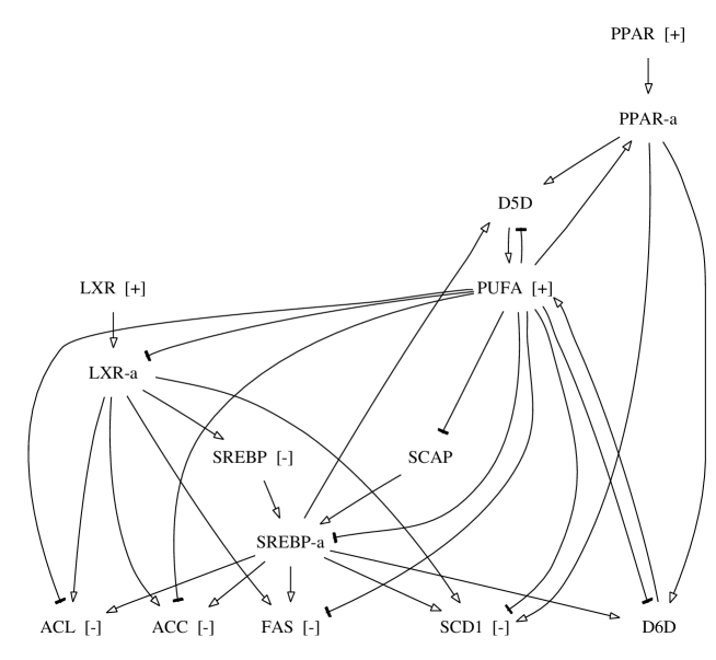
Figure 1: Interaction graph for the toy model. Self-regulation loops on nodes are omitted for sake of clarity. Observed variations are depicted next to each vertex, when available.

Variables in the model

We consider in our model nuclear receptors PPAR$\alpha$, LXR$\alpha$, SREBP-1c (denoted by PPAR, LXR, SREBP respectively in the model), as they are synthesized from the corresponding genes and the trans-activating active forms of these transcription factors, that is, LXR-a (denoting a complex LXR$\alpha$:RXR$\alpha$), PPAR-a (denoting a complex PPAR$\alpha$:RXR$\alpha$) and SREBP-a (denoting the cleaved form of SREBP-1c. We also consider SCAP – (SREBP cleavage activating protein), a key enzyme involved in the cleavage of SREBP-1c, that interacts with another family of proteins called INSIG (showing the complexity of molecular mechanism).

We also include in the model “final” products, that is, enzymes ACL, ACC, FAS, SCD1 (implied in the fatty acid synthesis from citrate), D5D, D6D (implied in PUFA synthesis) as well as PUFA themselves.

Interactions in the model

Relations between the variables are the following. SREBP-a is an activator of the transcription of ACL, ACC, FAS, SCD1, D5D and D6D [20, 13]. LXR-a is a direct activator of the transcription of SREBP and FAS, it also indirectly activates ACL, ACC and SCD1 [26]. Notice that these indirect actions are kept in the model because we don’t know whether they are only SREBP-mediated.

PUFA activates the formation of PPAR-a from PPAR, and inhibits the formation of LXR-a from LXR as well as the formation of SREBP-a (by inducing the degradation of mRNA and inhibiting the cleavage) [13]. SCAP represents the activators of the formation of SREBP-a from SREBP, and is inhibited by PUFA.

PPAR directly activates the production of SCD1, D5D, D6D [19, 27, 18]. The dual regulation of SCD1, D5D and D6D by SREBP and PPAR is paradoxical because SREBP transactivates genes for fatty acid synthesis in liver, while PPAR induces enzymes for fatty acid oxidation.
Hence, the induction of D5D and D6D gene by PPAR appears to be a compensatory response to the increased PUFA demand caused by induction of fatty acid oxidation.

Fasting-refeeding protocols

The fasting-refeeding protocols represent a favorable condition for studying lipogenesis regulation; we suppose that during an experimentation, animals (as rodents or chicken) were kept in a fasted state during several hours. Then, hepatic mRNA of LXR, SREBP, PPAR, ACL, FAS, ACC and SCD1 are quantified by DNA microarray analysis. Biochemical measures also provide the variation of PUFA.

A compilation of recent literature on lipogenesis regulation provides hypothetical results of such protocols: SREBP, ACL, ACC, FAS and SCD1 decline in liver during the fasted state [17]. This is expected because fasting results in an inhibition of fatty acid synthesis and an activation of the fatty acid oxidation. For the same reason, PPAR is increased in order to trigger oxidation. However, Tobin et al ([28]) showed that fasting rats for 24h increased the hepatic LXR mRNA, although LXR positively regulates fatty acid synthesis in its activated form. Finally, PUFA levels can be considered to be increased in liver following starvation because of the important lipolysis from adipose tissue as shown by Lee et al in mice after 72h fasting ([15]).

Qualitative system derived from the graph

As explained in the previous section, we derive a qualitative system from the interaction graph shown in Fig. 1. For ease of presentation, we denote by A the sign of variation for species A.

System 1

(1)  PPAR-a  = PPAR + PUFA
(2)  LXR-a   = -PUFA + LXR
(3)  SREBP   = LXR-a
(4)  SREBP-a = SREBP + SCAP -PUFA
(5)  ACL     = LXR-a + SREBP-a - PUFA
(6)  ACC     = LXR-a + SREBP-a - PUFA
(7)  FAS     = LXR-a + SREBP-a - PUFA
(8)  SCD1    = LXR-a  + SREBP-a - PUFA + PPAR-a
(9)  SCAP    = -PUFA
(10) D5D     = PPAR-a + SREBP-a - PUFA
(11) D6D     = PPAR-a + SREBP-a - PUFA

Observations 1

  PPAR    = +
  PUFA    = +
  LXR     = +
  SREBP   = -
  ACL     = -
  ACC     = -
  FAS     = -
  SCD1    = -

In the next section, we propose an efficient representation for such qualitative systems.

4 Analysis of qualitative equations: a new approach

4.1 Resolution of qualitative systems

The resolution of (even linear) qualitative systems is a NP-complete problem (see for instance [29, 8]). One can show this by reducing the satisfiability problem for a finite set of clauses to the resolution of a qualitative system in polynomial time.

Let us consider a collection $C=\{c_{1},\ldots,c_{n}\}$ of clauses on a finite set $V$ of variables. Let $\{\mbox{+},\mbox{\textminus},\mbox{?}\}$ a sign qualitative algebra. In order to reduce the satisfiability problem to the resolution of a qualitative system, let us code $true$ into $+$ and $false$ into $-$. If $c$ is a clause, let us denote by $\bar{c}$ the encoding of $c$ in a qualitative algebra formula. The following encoding scheme provides a polynomial procedure to code a clause into a qualitative formula. :

$$\begin{array}[]{ccc}\mbox{clause}&&\mbox{sign algebra}\\ \hline\cr a\in V&\rightarrow&\bar{a}\\ c_{1}\vee c_{2}&\rightarrow&\bar{c_{1}}+\bar{c_{2}}\\ \lnot c&\rightarrow&-\bar{c}\end{array}$$

The satisfiability problem for the set of clauses $C$ is then reduced to finding a solution of the qualitative system:

$$\{\bar{c_{i}}\approx\mbox{+}\ /\ i=1,\ldots,n\}$$

So a NP-complete problem can be reduced to the resolution of a qualitative system in polynomial time (with respect to the size of the problem). This shows that solving qualitative systems is a NP-complete problem. For example, the only pair of values which are not solution of $-\bar{a}+\bar{b}\ \approx\ +$ are $(+,-)$. This corresponds to the only pair $(true,false)$ that does not satisfy $\lnot a\vee b$.

Several heuristics were proposed for the resolution of qualitative systems. For linear systems, set of rules have been designed [8]. This set is complete: it allows to find every solution. It is also sound: every solution found by applying these rules is correct. The rules are based on an adaptation of Gaussian elimination. However only heuristics exist for choosing the equation and the rule to apply on it. In case of a dead-end, when no more rule can apply, it is necessary to backtrack to the last decision made. As a result programs implementing qualitative resolution are not very efficient in general and only problems of small size can be resolved in reasonable time. For that reason we propose an alternate way to solve qualitative systems (linear or not).

4.2 Qualitative equation coding

Our method is based on a coding of qualitative equations as algebraic equations over Galois fields ${\mathbb{Z}}/p{\mathbb{Z}}$ where $p$ is a prime number greater than 2. The elements of these fields are the classes modulo $p$ of the integers. If $\bar{x}$ denotes the class of the integer $x$ modulo $p$, a sum and a product are defined on ${\mathbb{Z}}/p{\mathbb{Z}}$ as follows:

$$\bar{x}+\bar{y}=\overline{x+y}\qquad\bar{x}\times\bar{y}=\overline{x\times y}$$

Galois fields have two basic properties which we use extensively:

• Every function $f:({\mathbb{Z}}/p{\mathbb{Z}})^{n}\rightarrow{\mathbb{Z}}/p{\mathbb{Z}}$ with $n$ arguments ${\mathbb{Z}}/p{\mathbb{Z}}$ is a polynomial function

• if $\oplus$ denotes the operation $f\oplus g=f^{(p-1)}+g^{(p-1)}$, then every equation system $p_{1}(X)=0,\ldots,p_{k}(X)=0$ has the same solutions than the unique equation $p_{1}\oplus p_{2}\oplus\ldots\oplus p_{k}(X)=0$.

The following table specifies how the sign algebra $\{\mbox{+},\mbox{\textminus},\mbox{?}\}$ is mapped onto the Galois field with three elements ${\mathbb{Z}}/3{\mathbb{Z}}$ is used for that coding.

$$\begin{array}[]{ccc}\mbox{sign algebra}&&\mathbb{Z}/3{\mathbb{Z}}\\ \hline\cr\mbox{+}&\rightarrow&1\\ \mbox{\textminus}&\rightarrow&-1\\ \mbox{?}&\rightarrow&0\\ \end{array}\qquad\qquad\qquad\begin{array}[]{ccc}\mbox{sign algebra}&&\mathbb{Z}/3{\mathbb{Z}}\\ \hline\cr e_{1}+e_{2}&\rightarrow&-\overline{e_{1}}.\overline{e_{2}}.(\overline{e_{1}}+\overline{e_{2}})\\ e_{1}\times e_{2}&\rightarrow&\overline{e_{1}}.\overline{e_{2}}\\ e_{1}\approx e_{2}&\rightarrow&\overline{e_{1}}.\overline{e_{2}}.(\overline{e_{1}}-\overline{e_{2}})\end{array}$$

Finally a qualitative system $\{e_{1},\dots,e_{n}\}$ is coded as the polynomial $\overline{e_{1}}\oplus\dots\oplus\overline{e_{n}}$. A similar coding for the qualitative algebra $\{\mbox{+},\mbox{\textminus},\mbox{0},\mbox{?}\}$ uses the Galois field ${\mathbb{Z}}/5{\mathbb{Z}}$ and will not be presented here.

With this coding, every qualitative system has a solution if and only if the corresponding polynomial has a solution without null component. Null solutions are excluded since ? solutions are excluded for qualitative systems. In general we will have to add polynomial equations $X^{2}=1$ to insure this.

4.3 An efficient representation of polynomial functions

Recall that our purpose is to efficiently solve a NP-complete problem. There is no hope to find a representation of polynomial functions allowing to solve polynomial systems of equations in polynomial time. The coding of a qualitative system as a polynomial equation is obviously polynomial in the size of the system (number of variables plus number of equations). So finding the solution of a polynomial system of equations is itself a NP-complete problem. It is more or less the SAT problem.

Nevertheless, there exists a representation of polynomial functions on Galois fields which gives, in practice, good performances for polynomials with hundreds of variables. This kind of representation was first used for logical functions which may be considered as polynomial functions over the field ${\mathbb{Z}}/2{\mathbb{Z}}$. This representation is known as BDD (Binary Decision Diagrams) and is widely used in checking logical circuits [2] and in model checkers as nu-SMV [5].

We present here this representation for the field ${\mathbb{Z}}/3{\mathbb{Z}}$. Generalizations to other Galois fields could be treated as well. The starting point is a generalization of Shannon decomposition for logical functions:

$$p(X_{1},X)=(1-X_{1}^{2})p_{[X_{1}=0]}(X)+X_{1}(-X_{1}-X_{1}^{2})p_{[X_{1}=1]}(X)+X_{1}(X_{1}-X_{1}^{2})p_{[X_{1}=2]}(X)$$

where $p$ is a polynomial function with $n$ variables. This decomposition leads to a tree representation of the polynomial function: the variable $X_{1}$ is the root and has three children. Each of these is obtained by instantiating $X_{1}$ to -1, 0 or 1 in $p(X_{1},X)$. This representation is exponential ($3^{n}$) as each non constant node has 3 children. It also depends on a chosen order on the variables.

Then a key observation (see [2]), is that several subtrees are identical. They have the same variable as root variable and isomorphic children. If we decide to represent only once each type of tree, then the tree representation is transformed into a direct acyclic graph. With this representation there is no more redundancy among subtrees. The result may be a dramatic decrease in the size of the representation of a polynomial function.

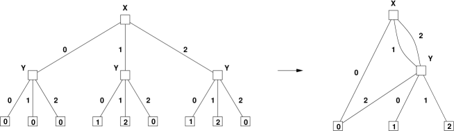
Figure 2: From tree representation to direct acyclic graph for $X^{2}(Y+1)$. The tree has 13 nodes while the DAG representing the same function has 5 nodes.

A property of the Shannon like decomposition is that many operations on polynomial functions are recursive with respect to this decomposition. More precisely let

$$p^{i}(X_{1},X)=(1-X_{1}^{2})p^{i}_{0}(X)+X_{1}(-X_{1}-X_{1}^{2})p^{i}_{1}(X)+X_{1}(X_{1}-X_{1}^{2})p^{i}_{2}(X)$$

$i=1,2$ be two polynomial functions with $p_{\alpha}(X)=p_{[X_{1}=\alpha]}(X)\ ,\ \alpha=0,1,2$. Then for binary operations $\Delta$ on polynomial functions,

$$p^{1}\Delta p^{2}=(1-X_{1}^{2})(p^{1}_{0}\Delta p^{2}_{0})+X_{1}(-X_{1}-X_{1}^{2})(p^{1}_{1}\Delta p^{2}_{1})+X_{1}(X_{1}-X_{1}^{2})(p^{1}_{2}\Delta p^{2}_{2})$$

This kind of recursive formula leads to an exponential complexity of any computation. Again, it is possible to take advantage of the redundancy by using a cache to remember each operation. This technique is known as memoisation in formal calculus. A 40% cache hit rate is commonly observed.

More complex operations on polynomial functions are also implemented with a recursive scheme and memoisation. Let us just mention quantifier elimination as among the most useful for our purpose.

This representation of polynomial functions on Galois fields has also several drawbacks:

• the memory size heavily depends on the order of variables. The libraries implementing formal computations always have reordering algorithms.

• for each order, there exists polynomial functions which are exponential in memory size.

Nevertheless, in practice, this representation has proved to be very efficient for polynomial functions with several hundred of variables. The computations performed on our toy model and on another real size one used a program named SIGALI which is devoted to polynomial functions on ${\mathbb{Z}}/3{\mathbb{Z}}$ representation. Several algorithms were added to this program in order to answer questions of biological interest.

5 Qualitative models and experimental data

In this section, we show how to compute some properties of a qualitative system, and eventually get some insights on the biological model it represents. The algorithms we derive heavily rely on the representation introduced above. Hence, not only they can deal in practice with computationally hard problems efficiently, but also they are expressed in a rather simple and generic fashion.

Let $M$ be a qualitative model represented by its associated interaction graph $G(V,E)$. Recall that $V$ is the set of variables. Let $V_{O}$ be the set of observed variables, and $o_{i}\in\{\mbox{+},\mbox{\textminus}\}$ for $i\in V_{O}$ the experimental observations. As explained in the previous section, the qualitative system derived from $M$ can be coded as a polynomial function $P_{M}(X_{1},\ldots,X_{n})$. Roots of $P_{M}$ correspond to solutions of the qualitative system.

5.1 Satisfiability of the qualitative system

A property of the coding described above, is that the system has no solution iff $P_{M}$ is equal to the constant polynomial $1$. Alternatively if $P_{M}=0$, the qualitative equations do not constraint the variables at all.

Now if some observations $o_{i}$ for $i\in V_{O}$ are available, checking their consistency with the model $M$ boils down to instantiating $X_{i}=o_{i}$ in $P_{M}(X_{1},\ldots,X_{n})$, for all $i\in V_{O}$, and testing whether the resulting polynomial is different from 1.

We computed the polynomial $P_{L}$ associated to our toy example (see section 3) and it has roots. Recall that it does not guarantee the existence of some (quantitative) differential model conforming to the interaction graph depicted in Fig. 1. Satisfiability of the qualitative system is only a necessary condition for the model to be correct.

The polynomial obtained by instantiating observations into $P_{L}$ is different from 1, meaning that our model does not contradict generally observed variations during fasting.

Large size models might advantageously be reduced using standard graph techniques. First we look for connected components in the interaction graph. A graph with several connected components represents a coherent qualitative model iff each component is coherent. Second, a node without successor except itself appears only in its associated equation. If this node is not observed, its associated qualitative equation adds no constraint on the other nodes. So, at least for satisfiability checking, this node can be suppressed and its qualitative equation removed from the system. This procedure is applied iteratively, until no node can be deleted. The resulting graph leads to a new qualitative system which is satisfiable iff the initial system is satisfiable.

5.2 Correcting data or model

If the qualitative system, given some experimental observations, is found to have no solution, it is of interest to propose some correction of the data and/or the model. By correction, we mean inverting the sign of an observed variable or the sign of an edge of the interaction graph. In the general case, there are several possibilities to make the system satisfiable, and we need some criterion to choose among them. We applied a parsimony principle: a correction of the data should imply a minimal number of sign inversions.

In the following, we show how to compute all minimal corrections for the data. Given $(o_{i})_{i\in V_{O}}$ a vector of experimental observations which is not compatible with the model, we compute all $(o^{\prime}_{i})_{i\in V_{O}}$ vectors which are compatible with the data and such that the Hamming distance between $o$ and $o^{\prime}$ is minimal. By Hamming distance, we mean the number of differences between $o$ and $o^{\prime}$. The set of such $o^{\prime}$ vectors might be very large; but again, by encoding it as the set of roots of a polynomial function, we obtain a compact representation.

This procedure can be extended in a straightforward manner to corrections of edges sign in the interaction graph. This is done by considering these signs as variables of the model. For ease of presentation, we only detail data correction.

Input:

  $P$, a polynomial function on variables $V$

  $i\in V$

Output:

  $C$, a polynomial function encoding all minimal corrections

  $d$, minimal number of corrections

if $P$ is constant then if $P$ = 0 then Result: $C=0$, $d=0$

else Result: $C=1$, $d=\infty$

end else let $P_{0}$, $P_{1}$, $P_{2}$ be the Shannon decomposition of $P$ with respect to variable $X_{i}$,

and $(C_{j},d_{j})$ the result obtained by recursively applying the algorithm on $P_{j}$ and $i+1$ for $j\in\{0,1,2\}$ let $d^{\prime}_{j}=\left\{\begin{array}[]{ll}d_{j}+1&\mbox{if }i\in V_{O}\mbox{ and }o_{i}\neq j\\ d_{j}&\mbox{otherwise}\end{array}\right.$ and $C^{\prime}_{j}=\left\{\begin{array}[]{ll}(X_{i}-j)\oplus C_{j}&\mbox{if }i\in V_{O}\\ C_{j}&\mbox{otherwise}\end{array}\right.$

Result: $d=\min\ d^{\prime}_{j}$, $C=\displaystyle\prod_{j,\ d^{\prime}_{j}=d}C^{\prime}_{j}$

end

Algorithm 1 Algorithm for experimental data correction.

Let us illustrate this algorithm on our toy example: during fasting experiments, synthesis of fatty acids tends to be inhibited, while oxidation, which produces ATP, is activated. In particular ACC, ACL, FAS and SCD1 are implied in the same pathway to produce saturated and monounsaturated fatty acids. Expectedly, they are known to decline together at fasting. Suppose we introduce some wrong observation, say for instance an increase of ACL, while keeping all other observations given above. The polynomial obtained from $P_{L}$ including these new observations is equal to 1, and hence has no solution. Applying algorithm 1, we recover this error. Now if we wrongly change two values, say ACL and ACC to 1, the algorithm proposes a different correction, namely to change the observed value of SREBP to 1, which is more parsimonious.

5.3 Experiment design

It is often the case that not all variables in the system under study can be observed. Biochemical measurements of metabolites can be costly and/or time consuming. By experiment design, we mean here the choice of the variables to observe so that an experiment might be informative.

Let $P_{M}(X_{O},X_{U})$ be the polynomial function coding for the qualitative system $M$. $X_{O}$ (resp. $X_{U}$) denotes the state vector of observed (resp. unobserved) variables. The polynomial function representing the admissible values of the observed variables is obtained by elimination of the quantifier in $\exists X_{U}\ P_{M}(X_{O},X_{U})$. Let $P_{M}^{O}(X_{O})$ denote the resulting polynomial function.

For some choice of observed variables, it might well be that $P_{M}^{O}$ is null, which basically means that the experiment is totally useless. Remark that no improvement can be found by taking a subset of $X_{O}$ The solution is either to add new observed variables or to chose a completely different set of observed variables.

In order to assess the relevance of a given experiment (namely of a given observed subset), we suggest to compute the following ratio: number of consistent valuations for observed variables versus the total number of valuations of observed variables. A very stringent experiment has a low ratio. An experiment having a ratio value of one is useless.

Again this computation is carried out in a recursive fashion. Let $P$ be a polynomial function representing the set of admissible observed values. Let $Rat(p)$ the percentage of solutions of $P(X)=0$ in the space $({\mathbb{Z}}/p{\mathbb{Z}})^{n}$, where $n$ is the number of variables $X$. If $P$ is constant then $Rat(P)=1$ (resp. $Rat(P)=0$) if $P=0$ (resp. $P\neq 0$). Else, let $P_{1}$, $P_{2}$, $P_{3}$ be a Shannon like decomposition of $P(X)$ with respect to some variable of $P$. Then it is easy to prove:

$$Rat(P)\ =\ (Rat(P_{0})+Rat(P_{1})+Rat(P_{2}))/3$$

The relevance of this approach was assessed on our toy example: for each subset $O$ of variables in the model, containing at most four variables, we computed $Rat(P_{L}^{O})$. Expectedly, the lowest ratios (i.e. the most stringent experiments) were achieved observing four variables: either {SCAP, PUFA, PPAR-a, PPAR}, or {SREBP, SCAP, PUFA, LXR-a}, or {SREBP, PPAR-a, PPAR, LXR-a}.

Interestingly, the procedure captures what might be though of as control variables, like PUFA/SCAP, SREBP/LXR-a and PPAR/PPAR-a. The first two pairs control the activation of fatty acids synthesis; the third one controls fatty acid oxidation.

Indeed one can go even further: if we isolate some kind of control variables, we are naturally interested in knowing how they constrain other variables. Achieving this amounts to computing the set of variables which value is constant for all solutions of the system (the so called hard components). Recall that these hard components of qualitative solutions are also important with respect to the hypothetical differential model which is abstracted in the qualitative one. Indeed, all solutions of the quantitative equation for equilibrium change have the same sign pattern on the hard components. Algorithm 2 describes a recursive procedure which finds the set of hard components, together with their value.

Input: $P$, a polynomial function on variables $V$

Output:

  the set $W\subset V\times\{0,1,2\}$ of hard components, together with their values

  a boolean $b$ which is true if $P$ has at least one root

if $P$ is constant then if $P$ = 0 then return $(\emptyset,\mbox{true})$ else return $(\emptyset,\mbox{false})$ end else let $P_{0}$, $P_{1}$, $P_{2}$ be the Shannon decomposition of $P$ with respect to variable $X_{i}$,

and $(W_{j},b_{j})$ the result obtained by recursively applying the algorithm on $P_{j}$ for $j\in\{0,1,2\}$ let $W=\{(v,v^{\prime})|v\in V,\ v^{\prime}\in\{0,1,2\},\ \forall j\ b_{j}\Rightarrow(v,v^{\prime})\in W_{j}\}$

if there exists a unique $j_{0}$ s.t. $b_{j_{0}}$ is true then add $(i,j_{0})$ to $W$ end return $(W,b_{0}\vee b_{1}\vee b_{2})$ end

Algorithm 2 Determination of hard components

Let us set some of our previously found control variables of the toy example, to a given value, say PUFA to 1, and LXR to -1. Then applying the algorithm 2, the corresponding polynomial has the following hard components:

ACL     = -1             FAS   = -1
ACC     = -1             LXR-a = -1
SCAP    = -1             SREBP = -1
SREBP-a = -1             PPAR  = -1
PPAR-a  = -1

which expectedly corresponds to the inhibition of fatty acids synthesis.

5.4 Real size system

We have used our new technique to check the consistency of a database of molecular interactions involved in the genetic regulation of fatty acid synthesis. In the database, interactions were classified as behavioral or biochemical.

• a behavioral interaction describes the effects of a variation of a product concentration. It is either direct or indirect (unknown mechanism).

• a biochemical interaction may be a gene transcription, a reaction catalyzed by an enzyme … Such molecular interactions can be found in existing databases. They need a behavioral interpretation.

All the behavioral interactions were manually extracted from a selection of scientific papers. Biochemical interactions were extracted from public databases available on the Web (Bind [1], IntAct [12], Amaze [16], KEGG [21] or TransPath [24]). A biochemical interaction may be linked to a behavioral interpretation in the database.

The database is used to generate the interaction graph. While behavioral interactions directly correspond to edges in the graph, biochemical interactions are given a simplified interpretation. Roughly, any increase of a reaction input induces an increase of the outputs.

The interaction graph which is built from the database contains more than 600 vertices and more than 1400 edges. It is clear that even though, the obtained graph is not a comprehensive model of genetic regulation of fatty acid synthesis in liver. Anyway our aim is to see how far this model can account for experimental observations, and propose some corrections when it cannot.

We used our technique to check the coherence of the whole model. After reducing the graph with standard graph techniques as described in section 5.1, we found that the model was incoherent. The reduced graph has about 150 nodes. We developed a heuristic to isolate minimal incoherent sub-systems. It turned out that all the contradictions we detected resulted from arguable interpretations of the literature.

6 Conclusion

In this paper we proposed a qualitative approach for the analysis of large biological systems. We rely on a framework more thoroughly described in [25], which is meant to model the comparison between two experimental conditions as a steady state shift. This approach fits well with state of the art biological measurement techniques, which provide rather noisy data for a large amount of targets. It is also well suited to the use of biological knowledge, which is most of the time descriptive and qualitative.

This qualitative approach is all the more attractive that we can rely on new analysis methods for qualitative systems. This new technique is also introduced in this paper and is original in qualitative modeling. It relies on a representation of qualitative constraints by decision diagrams. Not only this has a major impact on the scalability of qualitative reasoning, but it also permits to derive many algorithms in a quite generic fashion.

We plan to validate our approach on pathways which are published for yeast and E.Coli. Not only this pathways are of significant size but microarray data for this species are publicly available. Concerning the scalability of the methods, qualitative systems with up to 200 variables are handled within a few minutes.

On the theoretical side, we study applications of our algebraic techniques to network reconstruction, as proposed in [30]. The problem is to infer direct actions between products, based on large scale perturbation data, in order to obtain the most parsimonious interaction graph. Our approach could lead to a reformulation of this problem in terms of polynomial operations. Indeed, finding a minimal regulation network from a minimal polynomial representation has already been described in [14], though it was applied to a rather different type of network. A similar approach tailored to the framework described in this paper could eventually lead to original and practical algorithms for network reconstruction.

Acknowledgment

This research was supported by ACI IMPBio, a French Ministry for Research program on interdisciplinarity.

References

- [1] GD Bader, D Betel, and CW Hogue. Bind: the biomolecular interaction network database. Nucleic Acids Res., 31(1):248–50, 2003.
- [2] R.E Bryan. Graph-based algorithm for boolean function manipulation. IEEE Transactions on Computers, 8:677–691, August 1986.
- [3] Chaouiya C, Remy E, Ruet P, and Thieffry D. Qualitative modelling of genetic networks: From logical regulatory graphs to standard petri nets. Lecture Notes in Computer Science, 3099:137–156, 2004.
- [4] N. Chabrier-Rivier, M.Chiaverini, V. Danos, F. Fages, and V. Schächter. Modeling and querying biomolecular interaction networks. Theoretical Computer Science, 325(1):25–44, 2004.
- [5] E. Clarke, O. Grumberg, and D. Long. Verification tools for finite-state concurrent systems. in: A decade of concurrency - reflections and perspectives. Lecture Notes in Computer Science, 803, 1994.
- [6] H. de Jong. Modeling and simulation of genetic regulatory systems: A literature review. Journal of Computational Biology, 9(1):69–105, 2002.
- [7] H. de Jong, J.-L. Gouzé, C. Hernandez, M. Page, T. Sari, and J. Geiselmann. Qualitative simulation of genetic regulatory networks using piecewise-linear models. Bulletin of Mathematical Biology, 66(2):301–340, 2004.
- [8] J.L. Dormoy. Controlling qualitative resolution. In Proceedings of the seventh National Conference on Artificial Intelligence, AAAI88’, Saint-Paul, Minn., 1988.
- [9] David Fell. Understanding the Control of Metabolism. Portland Press, London, 1997.
- [10] Ronojoy Ghosh and Claire Tomlin. Symbolic reachable set computation of piecewise affine hybrid automata and its application to biological modelling: Delta-notch protein signalling. Systems Biology, 1(1):170–183, 2004.
- [11] Reinhart Heinrich and Stefan Schuster. The Regulation of Cellular Systems. Chapman and Hall, New York, 1996.
- [12] H. Hermjakob, L. Montecchi-Palazzi, C. Lewington, S. Mudali, and al. Intact – an open source molecular interaction database\̇lx@bibnewblockNucleic Acids Research, 32:D452–D455, 2004.
- [13] DB Jump. Fatty acid regulation of gene transcription. Crit. Rev. Clin. Lab. Sci., 41(1):41–78, 2004.
- [14] R. Laubenbacher and B. Stigler. A computational algebra approach to the reverse engineering of gene regulatory networks. J. Theor. Biol., 229:523–537, 2004.
- [15] SS Lee, WY Chan, CK Lo, and alt. Requirement of pparalpha in maintaining phospholipid and triacylglycerol homeostasis during energy deprivation. J Lipid Res., 45(11):2025–37, 2004.
- [16] C. Lemer, E. Antezana, F. Couche, and alt. The amaze lightbench: a web interface to a relational database of cellular processes. Nucleic Acids Res., 32:D443–D448, 2004.
- [17] G Liang, J Yang, JD Horton, RE Hammer, and alt. Diminished hepatic response to fasting/refeeding and liver x receptor agonists in mice with selective deficiency of sterol regulatory element-binding protein-1c. J Biol Chem, 277(15):9520–8, Jan 2002.
- [18] T Matsuzaka, H Shimano, N Yahagi, and alt. Dual regulation of mouse delta(5)- and delta(6)-desaturase gene expression by srebp-1 and pparalpha. J Lipid Res., 43(1):107–14, 2002.
- [19] CW Miller and JM Ntambi. Peroxisome proliferators induce mouse liver stearoyl-coa desaturase 1 gene expression. Proc Natl Acad Sci U S A., 93(18):9443–8, 1996.
- [20] TY Nara, WS He, C Tang, SD Clarke, and MT Nakamura. The e-box like sterol regulatory element mediates the suppression of human delta-6 desaturase gene by highly unsaturated fatty acids. Biochem. Biophys. Res. Commun., 296(1):111–7, 2002.
- [21] H. Ogata, S. Goto, K. Sato, W. Fujibuchi, and al. Kegg: Kyoto encyclopedia of genes and genomes. Nucleic Acids Research, 27:29–34, 1999.
- [22] O. Radulescu, S. Lagarrigue, A. Siegel, M. Le Borgne, and P. Veber. Topology and linear response of interaction networks in molecular biology. submitted to Royal Society Interface.
- [23] Gutierrez-Rios RM, Rosenblueth DA, Loza JA, Huerta AM, Glasner JD, Blattner FR, and Collado-Vides J. Regulatory network of escherichia coli: consistency between literature knowledge and microarray profiles. Genome Res., 13(11):2435–43, 2003.
- [24] F. Schacherer, C. Choi, U. Gotze, M. Krull, S. Pistor, and E. Wingender. The TRANSPATH signal transduction database: a knowledge base on signal transduction networks. Bioinformatics, 17(11):1053–1057, 2001.
- [25] A. Siegel, O. Radulescu, M. Le Borgne, P. Veber, J. Ouy, and S. Lagarrigue. Qualitative analysis of the relation between dna microarray data and behavioral models of regulation networks. Biosystems, submitted 2005.
- [26] KR Steffensen and JA. Gustafsson. Putative metabolic effects of the liver x receptor (lxr). Diabetes, 53(Supp 1):36–52, Feb 2004.
- [27] C Tang, HP Cho, MT Nakamura, and SD Clarke. Regulation of human delta-6 desaturase gene transcription: identification of a functional direct repeat-1 element. J Lipid Res, 44(4):686–95, 2003.
- [28] KA Tobin, HH Steineger, S Alberti, O Spydevold, and alt. Cross-talk between fatty acid and cholesterol metabolism mediated by liver x receptor-alpha. Mol Endocrinol, 14(5):741–52, May 2000.
- [29] L. Travé-Massuyès and P. Dague, editors. Modèles et raisonnements qualitatifs. Hermes sciences, 2003.
- [30] A. Wagner. Reconstructing pathways in large genetic networks from genetic perturbations. Journal of Computational Biology, 11:53–60, 2004.