A composite model for DNA torsion dynamics

Abstract

DNA torsion dynamics is essential in the transcription process; a simple model for it, in reasonable agreement with experimental observations, has been proposed by Yakushevich (Y) and developed by several authors; in this, the DNA subunits made of a nucleoside and the attached nitrogen bases are described by a single degree of freedom. In this paper we propose and investigate, both analytically and numerically, a “composite” version of the Y model, in which the nucleoside and the base are described by separate degrees of freedom. The model proposed here contains as a particular case the Y model and shares with it many features and results, but represents an improvement from both the conceptual and the phenomenological point of view. It provides a more realistic description of DNA and possibly a justification for the use of models which consider the DNA chain as uniform. It shows that the existence of solitons is a generic feature of the underlying nonlinear dynamics and is to a large extent independent of the detailed modelling of DNA. The model we consider supports solitonic solutions, qualitatively and quantitatively very similar to the Y solitons, in a fully realistic range of all the physical parameters characterizing the DNA.

I Introduction

The possibility that nonlinear excitations – in particular, kink solitons or breathers – in DNA chains play a functional role has attracted the attention of biophysicists as well as nonlinear scientists since the pioneering paper of Englander et al. Eng , and the works by Davydov on solitons in biological systems Dav .

A number of mechanical models of the DNA double chain have been proposed over the years, focusing on different aspects of the DNA molecule and on different biological, physical and chemical processes in which DNA is involved.

Here we will not discuss these, but just refer the reader to the discussions of such attempts given in the book by Yakushevich YakuBook and in the review paper by Peyrard PeyNLN (see also the conference PeyHouches ), also for what concerns earlier attempts which constituted the basis on which the models considered below were first formulated. Similarly, we will not describe the structure and functioning of DNA, but just refer e.g. to CD ; FK2 ; Sae . See also PeyHouches ; Pushchino for the role of Nonlinear Dynamics modelling in the understanding of DNA, and Lavery ; Strick for DNA single-molecule experiments (these were initiated about fifteen years ago SFB , but their range and precision has dramatically increased in recent years; the formation of bubbles in a double-stranded DNA has been observed in Lib ).

In recent years, two models have been extensively studied in the Nonlinear Physics literature; these are the model by Peyrard and Bishop PB (and the extensions of this formulated by Dauxois DauPLA and later on by Barbi, Cocco, Peyrard and Ruffo BCP ; BCPR ; see also Cocco and Monasson CM . More recent advances are discussed in PeyNLN and BLPT ; CuS ; TPM ) and the one by Yakushevich YakPLA ; we will refer to these as the PB and the Y models respectively.

Original versions of these models are discussed in GRPD ; they are put in perspective within a “hierarchy” of DNA models in YakPRE . An attempt to blend together the two is given in YakSBP ; see also Joy . Interplay between radial and torsional degrees of freedom is considered more organically in BCP ; BCPR .

The PB model is primarily concerned with DNA denaturation, and describes degrees of freedom related to “straight” (or “radial”) separation of the two helices which are wound together in the DNA double helical molecule. On the other hand, the Y model – on which we focus in this note – is primarily concerned with rotational and torsional degrees of freedom of the DNA molecule, which play a central role in the process of DNA transcription .

In this model, one studies a system of nonlinear equations which in the continuum limit reduce to a double sine-Gordon type equation; the relevant nonlinear oscillations are kink solitons – which are solitons in both dynamical and topological sense – which describe the unwinding of the double helix in the transcription region. The latter is a “bubble” of about 20 bases, to which RNA Polymerase (RNAP) binds in order to read the base sequence and produce the RNA Messenger; the RNAP travels along the DNA double chain, and so does the unwound region. The proposal of Englander et al. Eng was that if the nonlinear excitations are not created or forced by the RNAP but are anyway present due to the nonlinear dynamics of the DNA double helix itself, a number of questions – in particular, concerning energy flows – receive a simple explanation.

The Y model has been studied in a number of paper, in particular for what concerns its solitonic solutions; here we will quote in particular GaePLA1 ; GaePLA2 ; Gonz ; YakSBP ; YakPhD ; YakPRE . It has been shown that it gives a correct prediction of quantities related to small amplitude dynamics, such as the frequency of small torsional oscillations; as well as of quantities related to fully nonlinear dynamics, such as the size of solitonic excitations describing transcription bubbles GRPD ; YakuBook . Moreover, in its “helicoidal” version, it provides a scenario for the formation of nonlinear excitation out of linear normal modes lying at the bottom of the dispersion relation branches GRPD . On the other hand, if we try to fit the observed speed of waves along the chain YakuBook , this is possible only upon assuming unphysical values for the coupling constants YakPRE .

The Y model is also a very simple one, and adopts the same kind of simplification as in the PB model. In particular, two quite strong features of the models are:

• (a) there is a single (angular) degree of freedom for each nucleotide;

• $(b)$ all bases are considered as identical.

These were in a sense at the basis of the success of the model, in that thanks to these features the model can be solved exactly and one can check that predictions allowed by the model correspond to the real world situations for certain specific quantities. But the features mentioned above are of course not in agreement with the real situation.

Indeed, it is well known that bases are quite different from each other, and in particular purines are much bigger than pirimidines; hence feature (b) – albeit necessary for an analytical treatment of the model – is definitely unrealistic. Moreover, it is quite justified to consider several groups of atoms within a single nucleotide (the phosphodiester chain, the sugar ring, and the nitrogen base) as substantially rigid subunits; but these – in particular the sugar ring – have some degree of flexibility, and what’s more they have a considerable freedom of displacement – in particular for what concerns torsional and rotational movements – with respect to each other. Thus, even in a simple modelling, feature (a) is not justified per se, and it seems quite appropriate to consider several subunits within each nucleotide. In this sense, we will speak of a composite Yakushevich (Y) model. Needless to say, if such a more detailed modelling would produce results very near to those of the simple Y model, this should be seen as a confirmation that the latter correctly captures the relevant features of DNA torsional dynamics – hence justify a posteriori feature (a) of the Y model.

In this work we propose and study a composite Y model (in the sense mentioned above), in which we describe with two independent angular degrees of freedom, the nucleoside (i.e. the segment of the sugar-phosphate backbone pertaining to the nucleotide) and the nitrogen base in each nucleotide.

The purpose of our study of such a model is to shed light on the following points.

• (A) We want to take care (to some extent) of correcting feature (a) above and thus investigating – by comparing results – how justified is the original Y modelling in terms of one degree of freedom per nucleotide.

• (B) We aim at opening the way to correct – or justify – feature (b) of the Y model. Indeed, in our model we will consider separately the part of the nucleotide which precisely replicates identical in each nucleotide (the unit of the sugar-phosphate backbone), and the part which varies from one nucleotide to the other (the bases). We will then be able to study the different role of the two.

• (C) We want to check the dependence of the solitonic solution of the model both from the geometry and from the value of the physical parameters chosen. In particular, we would like to understand how far the existence of solitons is a generic feature of DNA and if a more realistic choice of the model geometry is consistent with phenomenologically acceptable values of the physical parameters.

It will turn out that the Y model, which can be considered as a particular case of our model, captures the essential features of DNA nonlinear dynamics. The more realistic geometry of the model we use in this paper enables a drastic improvement of the descriptive power of our model at both the conceptual and the phenomenological level: on the one hand the composite Y model keeps almost all the relevant features of the Y model, but on the other hand it allows for more realistic choice of the physical parameters.

It will turn out that the different degrees of freedom we use play a fundamentally different role in the description of DNA nonlinear dynamics. The backbone degrees of freedom are “topological” and play to some extent a “master” role, while those associated to the base are “nontopological” and are (in fluid dynamics language) “slaved” to former ones. This opens an interesting possibility, i.e. to consider a more realistic model, in which differences among bases are properly considered, as a perturbation of our idealized uniform model. As the essential features of the fully nonlinear dynamics are related only to backbone degrees of freedom, we expect that such a perturbation – albeit with relevant difference in the quantitative values of some parameters entering in the model (the base dynamical and geometrical parameters) – will show the same kind of nonlinear dynamics as our uniform model studied here.

The paper is organized as follows. In Sect. II we will briefly review some basic know facts about the DNA structure and modelling. In Sects. III and IV we will set up our model, describe the interaction and write down the equations of motions that govern its dynamics. The physical parameters characterizing our model are discussed in Sect. V. In Sect. VI we discuss the linear approximation of our dynamical system, in particular its dispersion relations. In Sect. VII we will set up the framework for the investigation of the nonlinear dynamics and the topological excitations of our model. In sect. VIII, we will show how the Y model and Y solitons emerge as a particular case of our composite Y model and its solitons. Sect. IX we investigate and derive numerically the solitonic solutions of our model. Finally in Sect. X we summarize our work and present our conclusions.

II DNA structure and modelling

DNA is a gigantic polymer, made of two helices wound together; the helices have a directionality and the two helices making a DNA molecule run in opposite direction. We will refer for definiteness to the standard conformation of the molecule (B-DNA); in this the pitch of the helix corresponds to ten base pairs, and the distance along the axis of the helix between successive base pairs is $\delta=3.4~{}\AA$.

The general structure of each helix can be described as follows. The helix is made of a sugar-phosphate backbone, to which bases are attached. The backbone has a regular structure consisting of repeated identical units (nucleosides); bases are attached to a specific site on each nucleoside and are of four possible types. These are either purines, which are adenine (A) or guanine (G), or pyrimidines, which are cytosine (C) or thymin (T) in DNA. It should be noted that the bases are rather rigid structures, and have an essentially planar configuration. A unit of each helix is called a nucleotide; this is the complex of a nucleoside and the attached base.

The winding together of the two helices makes that to each base site on the one helix corresponds a base site on the other helix. Bases at corresponding sites form a base pair; each base has only a possible partner in a base pair; bases in a pair are linked together via hydrogen bonds (two for A-T pairs, three for G-C pairs). The base pairs can be “opened” quite easily, the dissociation energy for each H-bond being of the order of 0.04 eV, hence $\Delta E\simeq 0.1$ eV per base pair. Opening is instrumental to a number of processes undergone by DNA, among which notably transcription, denaturation and replication.

The backbone structure (see Fig.1) is made of a phosphodiester chain and a sugar ring. To one of the $C$ atoms of the sugar ring is attached a base; this is one of the four possible bases $A,C,G,T$, whose sequence represents the information content of DNA and is different for different species, and to some extent for each individual. Thus, each helix is made of a succession of identical nucleosides, and attached bases which can be different at each site. Bases at corresponding sites on the two helices form a base pair, and these can be only of two types, G-C and A-T.

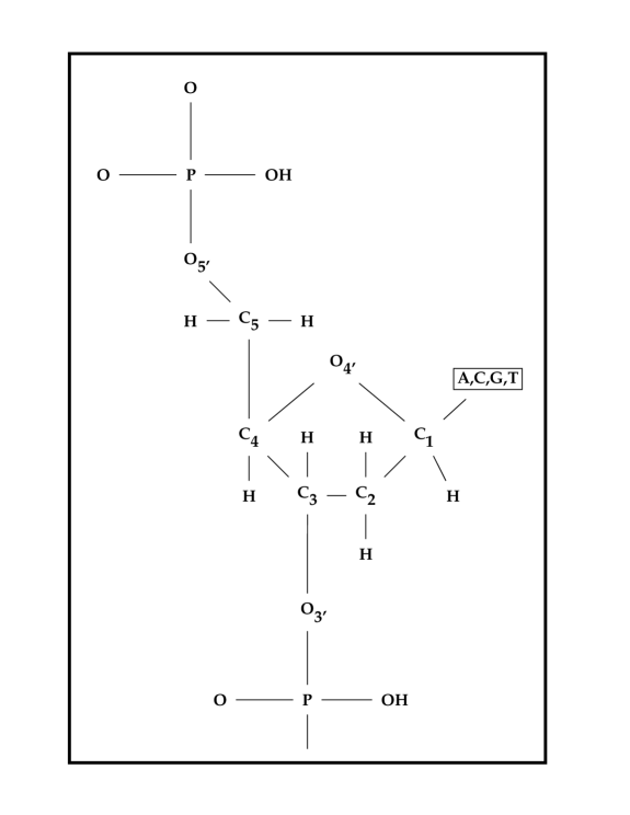
Figure 1: The structure of a DNA helix. A nucleotide is shown; nitrogen bases are attached to the $C_{1}$ atom in the sugar ring.

The atoms on each helix are of course held together by covalent bonds; apart from these, other interactions should be taken into account when attempting a description of the DNA molecule. The backbone structure has some rigidity; in particular, it would resist movements which represent a torsion of one nucleoside with respect to neighboring ones. We will refer to the interaction responsible for the forces resisting these torsion as torsional interactions.

As already mentioned, the two bases composing a base pair are linked together by hydrogen bonds; we will refer to the interaction mediated by these as pairing interaction. Each base interacts with bases at neighboring sites on the same chain via electrostatic forces (bases are strongly polar); these make energetically favorable the conformation in which bases are stacked on top of each other, and therefore are referred to as stacking interaction.

Finally, water filaments – thus, essentially, bridges of hydrogen bonds – link units at different sites; these are also known as Bernal-Fowler filaments Dav . In particular, they have a good probability to form between nucleosides or bases which are half-turn of the helix apart on different chains, i.e. which are near to each other in space due to the double helix geometry; these water filaments-mediated interactions are therefore also called helicoidal interactions . We stress that these are quite weaker than other interactions, and can be safely overlooked when we consider the fully nonlinear regime. They are instead of special interest when discussing small amplitude (low energy) dynamics, as – just because of their weakness – they are easily excited and introduce a length scale in the dispersion relations (see below).

If we consider large amplitude deviations from the equilibrium configurations, then motions will not be completely free: the molecule is densely packed, and the presence of the sugar-phosphate backbone – and of neighboring bases – will cause steric hindrances to the base movements. In particular, for the rotations in a plane perpendicular to the double helix axis, the bases will not be able to rotate around the $C_{1}$ atom for more than a maximum angle $\varphi_{0}$ without colliding with the nucleoside.

This will lead of course to complex behaviors as the DNA helix gets unwound; in particular, as $\varphi$ gets near to its limit value $\varphi_{0}$ we expect some kind of essentially (if not mathematically) discontinuous behavior. This should not be seen as shortcoming of the model: it is indeed well known that bases rotate in a complex way while flipping about the DNA axis (see e.g. Banavali ).

Finally, we mention that here we consider a DNA molecule without taking into account its macro-conformational features; that is, we consider an “ideal” molecule, disregarding supercoiling, organization in istones, and all that CD .

III Composite Y model

As mentioned above, we will model the molecule as made of different parts (units), each of them behaving as a single element, i.e. as a rigid body. We consider each nucleoside N as a unit, to which a base B (considered again as a single unit) is attached.

III.1 General features

We will hence model each of the helices in the DNA double chain as an array of elements (nucleotides) made of two subunits; one of these subunits model the nucleoside, the other the nitrogen base. We will consider the bases as all equal, thus disregarding the substantial difference between them . The chains – and thus the arrays – will be considered as infinite.

We will use a superscript $a=1,2$ to distinguish elements on the two chains, and a subscript $i\in{\bf Z}$ to identify the site on the chains. Thus the base pairing will be between bases $B_{i}^{(1)}$ and $B_{i}^{(2)}$, while stacking interaction will be between base $B_{i}^{(a)}$ and bases $B_{i+1}^{(a)}$ and $B_{i-1}^{(a)}$.

We will consider each nucleoside $N^{(a)}_{i}$ as a disk; bases will be seen as disks themselves, with a point on the border of $B^{(a)}_{i}$ attached via an inextensible rod to a point $p_{c}$ on the border of $N^{(a)}_{i}$; these points on B and N represent the locations of the $N$ atom on B and of the $C_{1}$ atom on N involved in the chemical bond attaching the base to the nucleoside. The rod can rotate by an angle $\pm\varphi_{0}$ before B collides with N; on the other hand, the disk N can rotate completely around its axis.

Figure 2: A base pair in our model. The origin of the coordinate system is in O. The angles $\theta_{1}$ between the lines AO and AB and $\theta_{2}$ between A’O and A’B’ correspond to torsion of sugar-phosphate backbone with respect to the equilibrium B-DNA conformation; the angles $\varphi_{1}$ between the line AB and the line BC, and $\varphi_{2}$ between A’B’ and B’C’ correspond to rotation of bases around the $C_{1}-N$ bond linking them to the nucleotide. All angles are in counterclockwise direction; thus the angles $\theta_{2}$ and $\varphi_{2}$ in the figure are negative.

We also single out a point $p_{h}$ on the border of the disk modelling the base; this represents the atom(s) which form the H bond with the corresponding base on the other DNA chain.

The disks (i.e. the elements of our model) are subject to different kinds of forces, corresponding to those described above: torsional forces resisting the rotation of one disk $N^{(a)}_{i}$ with respect to neighboring disks $N^{(a)}_{i+1}$ and $N^{(a)}_{i-1}$ on the same chain; stacking forces between a base $B_{i}^{(a)}$ and neighboring bases $B_{i+1}^{(a)}$ and $B_{i-1}^{(a)}$ on the same chain; pairing forces between bases $B_{i}^{(1)}$ and $B_{i}^{(2)}$ in the same base pair; and finally, helicoidal forces correspond to hydrogen bonded Bernal-Fowler filaments linking bases $B_{i}^{(1)}$ and $B_{i\pm 5}^{(2)}$ (and $B_{i}^{(2)}$ and $B_{i\pm 5}^{(1)}$).

III.2 The Lagrangian

We should now translate the above discussion into a Lagrangian defining our model. This will be written as

$$L\ =\ T\ -\ \left(U_{t}\ +\ U_{s}\ +\ U_{p}\ +\ U_{h}\right)$$ (III.1)

where $T$ is the kinetic energy, and $U_{a}$ are the potential energies for the different interactions listed above, i.e.

• $U_{t}$ is the backbone torsional potential,

• $U_{s}$ is the stacking potential,

• $U_{p}$ is the pairing potential,

• $U_{h}$ is the helicoidal potential.

These will be modelled by two-body potentials, for which we use the notation $V_{a}$, to be summed over all interacting pairs in order to produce the $U_{a}$.

We denote by $I$ the moment of inertia (around center of mass) of disks modelling the nucleosides, and by $I_{B}$ the moment of inertia of bases around the $C_{1}$ atom in the sugar ring; as the bases can not rotate around their center of mass, this is equal to $mr^{2}$, where $m$ is the base mass and $r$ is the distance between the $C_{1}$ atom in the sugar and the center of mass of the base.

III.3 The degrees of freedom

We are primarily interested in the torsional dynamics. Thus, for each element we will consider torsional movements, hence a rotation angle (with respect to the equilibrium conformation, which we take for definiteness to be B-DNA); these will be denoted as $\theta^{(a)}_{i}$ for the nucleoside $N^{(a)}_{i}$, and $\varphi^{(a)}_{i}$ for the base $B^{(a)}_{i}$. Only these rotations will be allowed in our model. All angles will be positive in counterclockwise sense.

The angles $\theta$ represent a torsion of the sugar-phosphate backbone with respect to the equilibrium configuration; thus they are related to unwinding of the double helix. On the other hand, the angles $\varphi$ represent a rotation of the base with respect to the corresponding nucleoside; the motion described by $\varphi$ can be thought of as a rotation around the $C_{1}$ atom in the sugar ring. Note that the hindrances due to the presence of backbone atoms constrain rotation of the base around the $C_{1}$ atom.

Thus, as mentioned above, the angles will have a different range of values:

$$\theta^{(a)}_{i}\in{\bf R}\ ,\ \ \varphi^{(a)}_{i}\in[-\varphi_{0},\varphi_{0}]\ \ \varphi_{0}<\pi\ .$$ (III.2)

The actual value of $\varphi_{0}$ is not essential. The important feature is that the base can not rotate freely around the $C_{1}$ atom, but only pivot between certain limits. At the level of the numerical analysis the simplest way to implement the previous boundary condition is to use a confining potential, which reproduces approximately the form of a box. For this reason in Sect. IX we will add to the Hamiltonian of the system a confining potential $V_{w}=K\tan^{4}\varphi^{(a)}$.

It should be stressed that – just on the basis of these different ranges of variations – there will be a substantial difference between the degrees of freedom described by the angles: those described by $\theta$ angles will be topological degrees of freedom, while those described by $\varphi$ angles will only describe local and (relatively) small motions – hence $\varphi$ describe non topological degrees of freedom.

III.4 Cartesian coordinates

In computing the kinetic energy, it will be convenient to consider cartesian coordinates. With reference to Fig. 2, the cartesian coordinates in the $(x,y)$ plane orthogonal to the double helix axis of relevant points will be as follow.

The center of disks, representing the position of the phosphodiester chain, will be $(x^{(a)}_{o},y^{(a)}_{o})$; the point on the border of the disks representing the $C_{1}$ atom to which the base disks are attached will be $(x^{(a)}_{c},y^{(a)}_{c})$. The center of mass of the bases will be $(x^{(a)}_{b},y^{(a)}_{b})$, and the point on the border of the disks modelling bases representing the atom(s) forming the H bonds will be $(x^{(a)}_{h},y^{(a)}_{h})$.

In terms of the $\{\theta,\varphi\}$ angles, these are given by (we omit the site index $i$ for ease of writing, and give condensed formulas for the two chains, with first sign referring to chain 1):

$$\begin{array}[]{ll}x^{(1,2)}_{o}=\mp a,&y^{(1,2)}_{o}=0;\\ x^{(1,2)}_{c}=x^{(1,2)}_{o}\pm R\cos(\theta^{(1,2)}),&y^{(1,2)}_{c}=\pm R\sin(\theta^{(1,2)});\\ x^{(1,2)}_{b}=x^{(1,2)}_{c}\pm r\cos(\theta^{(1,2)}+\varphi^{(1,2)}),&y^{(1,2)}_{b}=y^{(1,2)}_{c}\pm r\sin(\theta^{(1,2)}+\varphi^{(1,2)});\\ x^{(1,2)}_{h}=x^{(1,2)}_{c}\pm d_{h}\cos(\theta^{(1,2)}+\varphi^{(1,2)}),&y^{(1,2)}_{h}=y^{(1,2)}_{c}\pm d_{h}\sin(\theta^{(1,2)}+\varphi^{(1,2)}).\\ \end{array}$$ (III.3)

Here and in the following we denote by $R$ the radius of disks describing nucleosides, i.e. the length of the segments AB and A’B’ in Fig. 2 (this is the distance from the phosphodiester chain to the $C_{1}$ atom); by $r$ the distance between the center of mass of bases and the border of the disk modelling the nucleoside (i.e. the $C_{1}$ atom). We also denote by $d_{h}$ the lengths (supposed equal) of the segments BC and B’C’ joining the $C_{1}$ atom on the nucleoside and the atoms of the bases forming the hydrogen bond linking this to the complementary base. The parameter $a$ corresponds to the distance between the double helix axis and the phosphodiester chain, whereas $\rho_{0}$ is the distance between points $C$ and $C^{\prime}$ in the equilibrium configuration. The previous parameters are obviously related by the equation $2a=2R+2d_{h}+\rho_{0}$.

III.5 Kinetic energy

With this notation, and standard computations, the kinetic energy of each nucleotide is written as

$$T_{i}^{(a)}=\frac{1}{2}\left[mr^{2}{\dot{\varphi}}^{2}+2mr(r+R\cos\varphi){\dot{\theta}}{\dot{\varphi}}+\left(I+m_{B}(R^{2}+r^{2})+2mRr\cos\varphi\right){\dot{\theta}}^{2}\right],$$

where we have suppressed super- and sub-scripts for ease of reading. Thus, the total kinetic energy for the double chain is

$$\begin{array}[]{rl}T\ =&\ \sum_{a}\ \sum_{i}\ T^{(a)}_{i}\ =\\ =&\ \frac{1}{2}\,\sum_{a}\sum_{i}\ \left[m\,r^{2}\,\left({\dot{\varphi}}^{(a)}_{i}\right)^{2}\ +\ 2\,m\,r\,(r+R\cos(\varphi^{(a)}_{i}))\,{\dot{\theta}}^{(a)}_{i}\,{\dot{\varphi}}^{(a)}_{i}\ +\right.\\ &\left.+\ \left(I+m_{B}(R^{2}+r^{2})+2mRr\cos(\varphi^{(a)}_{i})\right)\left({\dot{\theta}}^{(a)}_{i}\right)^{2}\right]\ \ .\end{array}$$ (III.4)

We have thus considered a general class of composite Y models; so far we have not specified the interaction potentials, which are needed to have a definite model.

III.6 Modelling the interactions

We have now to specify our model by fixing analytical expressions for terms modelling potential interactions in the lagrangian (III.1). As one of our aims is to compare the results obtained by a composite Y model with those obtained with the simple Y model, we will make choices with the same physical content as those made by Yakushevich.

III.6.1 Torsional interactions

Torsional forces will depend only on difference of angles (measured with respect to the equilibrium B-DNA configuration) of neighboring units on the same phosphodiester chain; thus we introduce a torsion potential $V_{t}$ and have

$$U_{t}\ =\ \sum_{a}\sum_{i}V_{t}\left(\theta^{(a)}_{i+1}-\theta^{(a)}_{i}\right)\ .$$ (III.5)

The potential $V_{t}$ must have a minimum in zero, and be $2\pi$-periodic in order to take into account the fundamentally discrete and quantum nature of the phosphodiester chain. Here we will take the simplest such function , i.e. (adding an inessential constant so that the minimum corresponds to zero energy)

$$V_{t}(x)\ =\ K_{t}\left(1\ -\ \cos(x)\right)$$ (III.6)

where $K_{t}$ is a dimensional constant. Thus, our choice for torsional interactions will be

$$U_{t}\ =\ K_{t}\ \sum_{a}\sum_{i}\,\left[1\,-\,\cos\left(\theta^{(a)}_{i+1}-\theta^{(a)}_{i}\right)\right]\ .$$ (III.7)

The harmonic approximation for this is of course

$$U_{t}^{q}\ =\frac{1}{2}K_{t}\ \sum_{a}\sum_{i}\,\left(\theta^{(a)}_{i+1}-\theta^{(a)}_{i}\right)^{2}\ .$$

III.6.2 Stacking interactions

Stacking between bases will only depend on the relative displacement of neighboring bases on the same helix in the plane orthogonal to the double helix axis . That is, introducing a stacking potential $V_{s}$ we have

$$U_{s}\ =\ \sum_{a}\sum_{i}V_{s}\left(\sigma^{(a)}_{i}\right)\ ,$$ (III.8)

where

$$\sigma^{(a)}_{i}\ :=\ \sqrt{(x^{(a)}_{i+1}-x^{(a)}_{i})^{2}\ +\ (y^{(a)}_{i+1}-y^{(a)}_{i})^{2}}\ ,$$ (III.9)

where $x^{(a)}_{i},\,y^{(a)}_{i}$ are the coordinates of the center of mass of the bases. The simplest choice corresponds to a harmonic potential , $V_{s}=(1/2)K_{s}\sigma^{2}$. This will be our choice – which again corresponds to the one made in the PB and in the Y models, so that

$$U_{s}\ =\ \sum_{a}\sum_{i}\frac{K_{s}}{2}\,(\sigma^{(a)}_{i})^{2}\ .$$ (III.10)

We should however express this in terms of the $\theta$ and $\varphi$ angles. With standard algebra, using Eqs. (III.3), we obtain

$$\begin{array}[]{rl}U_{s}\ =&\ \frac{1}{2}\,K_{s}\ \sum_{a}\sum_{i}\ 2\,\left[R^{2}+r^{2}\ +\right.\\ &\left.-\ R^{2}\cos(\theta^{(a)}_{i+1}-\theta^{(a)}_{i})\,-\,r^{2}\cos[(\theta^{(a)}_{i+1}-\theta^{(a)}_{i})+(\varphi^{(a)}_{i+1}-\varphi^{(a)}_{i})]\ +\right.\\ &\left.-\ Rr\left(\cos[(\theta^{(a)}_{i+1}-\theta^{(a)}_{i})+\varphi^{(a)}_{i+1}]+\cos[(\theta^{(a)}_{i+1}-\theta^{(a)}_{i})-\varphi^{(a)}_{i}]\right)\ +\right.\\ &\left.+\ Rr\left(\cos(\varphi^{(a)}_{i+1})+\cos(\varphi^{(a)}_{i})\right)\right]\ .\end{array}$$ (III.11)

III.6.3 Pairing interactions

Pairing interactions are due to stretching of the hydrogen bonds linking bases in a pair. Introducing a paring potential $V_{p}$ which models the H bonds, we have

$$U_{p}\ =\ \sum_{i}\,V_{p}(\theta^{(1)}_{i},\theta^{(2)}_{i},\varphi^{(1)}_{i},\varphi^{(2)}_{i})\ .$$ (III.12)

We note that H bonds are strongly directional, so that they are quickly disrupted once the alignment between pairing bases is disrupted. This feature is traditionally disregarded in the Y model, where it is assumed that $V_{p}$ only depends on the distance

$$\rho_{i}\ :=\sqrt{(x^{(1)}_{i}-x^{(2)}_{i})^{2}+(y^{(1)}_{i}-y^{(2)}_{i})^{2}}$$ (III.13)

between the interacting bases; that is,

$$U_{p}\ =\ \sum_{i}\,V_{p}(\rho_{i})\ .$$ (III.14)

As noted by Gonzalez and Martin-Landrove Gonz in the context of the Yakushevich model, one should be careful in expanding a potential $V_{p}(\rho)$ in terms of the rotation angles $\varphi$ and $\theta$: indeed, unless $\rho_{0}=0$, i.e. $a=R+d_{h}$, one would get zero quadratic term in such an expansion (see however GaeY1 for what concerns solitons in this context).

As for the potential $V_{p}$, there are two simple choices for this appearing in the literature. On the one hand, Yakushevich YakPLA suggests to consider a potential harmonic in the intrapair distance $\rho$ (this would appear nonlinear when expressed through rotation angles) and this has been kept in subsequent discussions and extensions of her model YakuBook ; on the other hand, Peyrard and Bishop PB consider a Morse potential; again this has been kept in subsequent discussions and extensions of their model PeyNLN .

There is no doubt that the Morse potential is more justified in physical terms; however, as we wish to compare our results with those of the original Y model, we will at first consider a harmonic potential

$$V_{p}^{(Y)}(\rho)\ =\ \frac{1}{2}\,K_{p}\,(\rho-\rho_{0})^{2}\ ,$$ (III.15)

where $\rho_{0}$ is the intrapair distance in the equilibrium configuration. Moreover, again in order to compare our results with those of the original Y model, we will later on set $\rho_{0}=0$. This corresponds to setting $a=R+d_{h}$. These approximations can appear very crude, but experience gained (as preliminary work for the present investigation) with the standard Yakushevich model GaeY1 ; GaeY2 suggests they do not have a great impact at the level of fully nonlinear dynamics.

We should express $V_{p}$ in terms of the rotations angles. Using once again the expressions (III.3), we have with standard computations that

$$\begin{array}[]{rl}\rho_{i}^{2}\ :=&\left(x^{(1)}_{i}-x^{(2)}_{i}\right)^{2}\ +\ \left(y^{(1)}_{i}-y^{(2)}_{i}\right)^{2}\ =\\ =&2\left[2a^{2}+R^{2}+d_{h}^{2}+R^{2}\cos(\theta^{(1)}_{i}-\theta^{(2)}_{i})+d_{h}^{2}\cos[(\theta^{(1)}_{i}-\theta^{(2)}_{i})+(\varphi^{(1)}_{i}-\varphi^{(2)}_{i})+\right.\\ &\left.+\ Rd_{h}\left(\cos\varphi^{(1)}_{i}+\cos\varphi^{(2)}_{i}+\cos[(\theta^{(1)}_{i}-\theta^{(2)}_{i})+\varphi^{(1)}_{i}]+\cos[(\theta^{(1)}_{i}-\theta^{(2)}_{i})-\varphi^{(2)}_{i}]\right)+\right.\\ &\left.-2aR\left(\cos(\theta^{(1)}_{i})+\cos(\theta^{(2)}_{i})\right)-2ad_{h}\left(\cos(\varphi^{(1)}_{i}+\theta^{(1)}_{i})+\cos(\varphi^{(2)}_{i}+\theta^{(2)}_{i})\right)\right]\ .\end{array}$$ (III.16)

With this, our choice for the pairing part of the hamiltonian will be

$$U_{p}\ =\ \sum_{i}\,V_{p}(\rho_{i})\ .$$ (III.17)

III.6.4 Helicoidal interactions

Helicoidal interaction are mediated by water filaments (Bernal-Fowler filaments Dav ) connecting different nucleotides; in particular we will consider those being on opposite helices at half-pitch distance, as they are near enough in three-dimensional space due to the double helical geometry. As the nucleotide move, the hydrogen bonds in these filaments – and those connecting the filaments to the nucleotides – are stretched and thus resist differential motions of the two connected nucleotides.

We will, for the sake of simplicity and also in view of the small energies involved, only consider filaments forming between nucleosides; thus only the $\theta$ angles will be involved in these interactions. We have therefore, introducing a helicoidal potential $V_{h}$ and recalling that the pitch of the helix corresponds to 10 bases in the B-DNA equilibrium configuration,

$$U_{h}\ =\ \sum_{i}\,V_{h}(\theta^{(1)}_{i+5}-\theta^{(2)}_{i})\ +\ V_{h}(\theta^{(2)}_{i+5}-\theta^{(1)}_{i})\ .$$ (III.18)

As the angles $\theta$ are involved, the potential $V_{h}$ should be $2\pi$-periodic .

Such water filament connections involve a large number (around 10) of hydrogen bonds; hence each of them is only slightly stretched, and it makes sense to consider the angular-harmonic approximation

$$V_{h}(\tau)\ =\ K_{h}[1-\cos(\tau)]\ \simeq\ \frac{1}{2}K_{h}\tau^{2}\ .$$ (III.19)

Our choice will therefore be

$$U_{h}\ =\ K_{h}\,\sum_{i}\,\left[2-\cos(\theta^{(1)}_{i+5}-\theta^{(2)}_{i})-\cos(\theta^{(2)}_{i+5}-\theta^{(1)}_{i})\right]\ .$$ (III.20)

IV Equations of motion

In the previous sections we have set up the model and the interactions. Let us now study its dynamics. We denote collectively the variables as $\psi^{a}$, e.g. with $\psi=(\varphi^{(1)},\varphi^{(2)},\theta^{(1)},\theta^{(2)})$. The dynamics of the model will be described by the Euler-Lagrange equations corresponding to the Lagrangian (III.1) with the terms in the interaction potential given respectively by Eqs. (III.7), (III.11), (III.17), (III.20)

$$\frac{\partial L}{\partial\psi^{a}_{i}}\ -\ \frac{{\rm d}}{{\rm d}t}\frac{\partial L}{\partial{\dot{\psi}}^{a}_{i}}\ =\ 0\ .$$ (IV.1)

With our choices for the different terms of $L$, and writing $\hat{a}$ for the complementary chain of the chain $a$ (that is, $\hat{1}=2$, $\hat{2}=1$), these read

$$\begin{array}[]{l}mr^{2}{\ddot{\varphi}}^{(a)}_{i}+mr[R\cos(\varphi^{(a)}_{i})+r]{\ddot{\theta}}^{(a)}_{i}+mrR\sin(\varphi^{(a)}_{i})({\dot{\theta}}^{(a)}_{i})^{2}\ =\\ \ =\ K_{s}r^{2}\sin[\varphi^{(a)}_{i-1}-\varphi^{(a)}_{i}+\theta^{(a)}_{i-1}-\theta^{(a)}_{i}]-2ad_{h}K_{p}\sin(\varphi^{(a)}_{i}+\theta^{(a)}_{i})\\ -K_{s}rR\sin(\varphi^{(a)}_{i}-\theta^{(a)}_{i-1}+\theta^{(a)}_{i})-K_{s}rR\sin(\varphi^{(a)}_{i}+\theta^{(a)}_{i}-\theta^{(a)}_{i+1})\\ \ \ \ -K_{s}r^{2}\sin(\varphi^{(a)}_{i}-\varphi^{(a)}_{i+1}+\theta^{(a)}_{i}-\theta^{(a)}_{i+1})+d_{h}K_{p}R\sin(\varphi^{(a)}_{i}+\theta^{(a)}_{i}-\theta^{(\hat{a})}_{i})+\\ d_{h}^{2}K_{p}\sin(\varphi^{(a)}_{i}-\varphi^{(\hat{a})}_{i}+\theta^{(a)}_{i}-\theta^{(\hat{a})}_{i})+R(d_{h}K_{p}+2K_{s}r)\sin[\varphi^{(a)}_{i}]\ ;\\ {}\\ mrR\cos(\varphi^{(a)}_{i})({\ddot{\varphi}}^{(a)}_{i}+2{\ddot{\theta}}^{(a)}_{i})+mr^{2}{\ddot{\varphi}}^{(a)}_{i}+I{\ddot{\theta}}^{(a)}_{i}+mr^{2}{\ddot{\theta}}^{(a)}_{i}+mR^{2}{\ddot{\theta}}^{(a)}_{i}\\ -mrR\sin(\varphi^{(a)}_{i}){\dot{\varphi}}^{(a)}_{i}({\dot{\varphi}}^{(a)}_{i}+2{\dot{\theta}}^{(a)}_{i})\ =\\ \ =\ (K_{t}+K_{s}R^{2})\sin(\theta^{(a)}_{i-1}-\theta^{(a)}_{i})+K_{s}rR\sin(\varphi^{(a)}_{i-1}-(\theta^{(a)}_{i}-\theta^{(a)}_{i-1}))\\ -K_{s}r^{2}\sin((\varphi^{(a)}_{i}-\varphi^{(a)}_{i-1})\ \ \ +(\theta^{(a)}_{i}-\theta^{(a)}_{i-1}))-2aK_{p}R\sin(\theta^{(a)}_{i})-\\ 2ad_{h}K_{p}\sin(\varphi^{(a)}_{i}+\theta^{(a)}_{i})-K_{s}rR\sin[\varphi^{(a)}_{i}+(\theta^{(a)}_{i}-\theta^{(a)}_{i-1})]\\ -K_{s}rR\sin(\varphi^{(a)}_{i}-(\theta^{(a)}_{i+1}-\theta^{(a)}_{i}))+(K_{t}+K_{s}R^{2})\sin(\theta^{(a)}_{i+1}-\theta^{(a)}_{i})\\ +K_{s}r^{2}\sin[(\varphi^{(a)}_{i+1}-\varphi^{(a)}_{i})+(\theta^{(a)}_{i+1}-\theta^{(a)}_{i})]+K_{s}rR\sin[\varphi^{(a)}_{i+1}+(\theta^{(a)}_{i+1}-\theta^{(a)}_{i})]+\\ K_{p}R^{2}\sin(\theta^{(a)}_{i}-\theta^{(\hat{a})}_{i})+d_{h}K_{p}R\sin(\varphi^{(a)}_{i}+(\theta^{(a)}_{i}-\theta^{(\hat{a})}_{i}))\ \ \ +\\ d_{h}^{2}K_{p}\sin((\varphi^{(a)}_{i}-\varphi^{(\hat{a})}_{i})+(\theta^{(a)}_{i}-\theta^{(\hat{a})}_{i}))-d_{h}K_{p}R\sin(\varphi^{(\hat{a})}_{i}-(\theta^{(a)}_{i}-\theta^{(\hat{a})}_{i}))\\ +K_{h}\left(\theta^{(\hat{a})}_{i+5}-2\theta^{(a)}_{i}+\theta^{(\hat{a})}_{i-5}\right)\end{array}$$ (IV.2)

Note that here $a,R,r,d_{h}$ are considered as independent parameters, i.e. we have not enforced the Yakushevich condition $R+d_{h}=a$ (i.e. $\rho_{0}=0$). Needless to say, these are far too complex to be analyzed directly, and we will need to introduce various kinds of approximation.

We have thus completely specified the model we are going to study and derived the equations that govern its dynamics, i.e. its lagrangian and the equations of motion. The choice of torsion angles as variables to describe our dynamics led to involved expressions, but our choices are very simple physically.

We have considered “angular harmonic” approximations (expansion up to first Fourier mode) i.e. potentials of the form $V(x)=[1-\cos(x)]$ for the torsion and helicoidal interactions, harmonic approximation for the base stacking interaction, and a harmonic potential depending on the intrapair distance for the pairing interaction. Our approximations are coherent with those considered in the literature when dealing with uniform models of the DNA chain, and in particular when dealing with (extensions of) the Yakushevich model. Thus, when comparing the characteristic of our model with those of these other models, we are really focusing on the differences arising from considering separately the nucleoside and the base within each nucleotide.

It would of course be possible to consider more realistic expressions for the potentials; but we believe that at the present stage this would rather obscure the relevant point here, i.e. the discussion of how such “composite” models can retain the remarkable good features of the Y model and at the same time overcome some of the difficulties they encounter. Finally, we note that it is quite obvious that the dynamical equations describing the model are – despite the simplifying assumptions we made at various stage – too hard to have any hope to obtain a general solution, either in the discrete or in the continuum version (see below) of the model.

In the next section we will focus our attention on the choice of the physical parameters appearing in our model. Later, we will investigate the dynamics beginning with the linear approximation and then in the fully nonlinear regime.

V Physical values of parameters

In order to have a well defined model we should still assign concrete values to the parameters – both geometrical ones and coupling constants – appearing in our Lagrangian (III.1) and in the equation of motion (IV.2).

V.1 Kinematical parameters

Let us start by discussing kinematical parameters; in these we include the geometrical parameters as well as the mass $m$ and the moment of inertia $I$.

The masses can be readily evaluated by considering the chemical structure of the bases. They can be calculated just by knowing masses of the atoms and their multiplicity in the different bases. As for the geometrical parameters like $R$, $a$, $r$ and $d_{h}$ (and the moment of inertia $I$), quite surprisingly different authors seem to provide different values for these. Rather than assuming the values given by one or another author, we have preferred to estimate the parameters using the available information about the DNA structure. Position of atoms within the bases (which of course determine $R$, $a$, $r$ and $d_{h}$, and hence $I$) and geometrical descriptions of DNA are widely available to the scientific community in form of PDB files PDBRep . We will use this information (which we accessed at 1BNA and PDBFiles ) to estimate directly all static parameters in play on the basis of the atomic positions.

The geometrical parameters which are relevant for our discussion are the longitudinal width of bases $l_{b}$ and of the sugar $l_{s}$, the distances of the bases from the relative sugars $d_{s}$ and the distance of a base from the relative dual base $d_{b}$. We give our estimates for the masses, moments of inertia and the parameters $l,d_{s},d_{b}$ for the different bases and their mean values in Table 1. ¿From those data and using the equations $R=l_{s},\,r={\hat{d}}_{s}+{\hat{l}}_{b}/2,\,d_{h}={\hat{l}}_{b}+{\hat{d}}_{s},\,a=l_{s}+{\hat{l}}_{b}+{\hat{d}}_{s}+{\hat{d}}_{b}/2$ (hats denote mean values), one obtains the average values for the geometrical parameters appearing in our Lagrangian. given in table 2.

	A	T	G	C	mean	Sugar
$m$	134	125	150	110	130	85
$I$	$3.6\times 10^{3}$	$3.0\times 10^{3}$	$4.4\times 10^{3}$	$2.3\times 10^{3}$	$3.3\times 10^{3}$	$1.2\times 10^{2}$
$l$	$3.2$	$4.0$	$5.0$	$2.4$	$4.7$	$3.3$
$d_{s}$	$1.5$	$1.5$	$1.5$	$1.5$	$1.5$	-
$d_{b}$	$2.0$	$2.0$	$2.0$	$2.0$	$2.0$	-

Table 1: Order of magnitude for the basic geometrical parameters of the DNA. Units of measure are: atomic unit for masses $m$, $1.67\times 10^{-47}{\rm Kg}\cdot{\rm m}^{2}$ for the inertia momenta $I$, Angstrom for $l$, $d_{s}$ and $d_{b}$, respectively the longitudinal width of bases and their distances from the relative sugars and from the relative dual base. These values have been extracted from the sample “generic” B-DNA PDB data PDBFiles , kindly provided by the Glactone Project Glac , and double checked with the data from 1BNA , that agree within $5\%$. Inertia momenta of bases has been evaluated with respect to rotations about the DNA’s symmetry axis passing through the sugar’s $C_{1}$ atom the base is attached to; the inertia momentum of the sugar itself has been evaluated with respect to rotations about its $C_{3}-C_{4}$ axis (see Fig. 1)

$R$	$r$	$d_{h}$	$a$
3.3 Å	3.8 Å	6.2 Å	10.5 Å

Table 2: Numerical values of the geometrical parameters chracterizing our model

V.2 Coupling constants

The determination of the four coupling constants appearing in our model is more problematic, due partly to the difficulties in making experiments to test single coupling constants and partly to the complexity of the system itself.

V.2.1 Pairing

The coupling constant $K_{p}$, which appears in the pairing potential (III.17) can be easily determine by considering the typical energy of hydrogen bonds. The pairing interaction involves two (in the $A-T$ case) or three (in the $G-C$ case) electrostatic hydrogen bond. The pairing potential can be modelled with a Morse function

$$V_{p}(x)=D(e^{-bd(x,x_{0})}-1)^{2}=\frac{1}{2}(2Db^{2})(\rho-\rho_{0})^{2}+O(\rho^{3})\,,$$ (V.1)

where $D$ is the potential depth, $\rho$ the distance from the equilibrium position $\rho_{0}$ and $b$ a parameter that defines the width of the well. Although throughout this paper we use the harmonic potential (III.17) to model the pairing interaction, the use of the Morse function seems more appropriate for evaluating the parameter $K_{p}$. The point is that the pairing coupling constant is physically determined by the behavior of the pairing potential away from its minimum. Using the harmonic approximation (III.17) for estimate $K_{p}$ would result in a completely unphysical value for the parameter.

Different estimates of the parameters appearing in the potential (V.1) are present in the literature. The estimates

$$D_{AT}=0.030{\rm eV},\ D_{GC}=0.045{\rm eV},\ b_{AT}=1.9{\rm\AA}^{-1},\ b_{GC}=2.5{\rm\AA}^{-1}$$

are given in CP and used in ZC . The values

$$D=0.040{\rm eV},\ b=4.45{\rm\AA}^{-1}$$

are given in PBD and used in PBD ; BCP ; DeLuca . Finally, the estimates

$$D_{AT}=0.050{\rm eV},\ D_{GC}=0.075{\rm eV},\ b_{AT}=b_{GC}=4{\rm\AA}^{-1}$$

are given in Campa and used in Campa ; KS . The values of coupling constants corresponding to these different values for the parameters appearing in the Morse potential range across a whole order of magnitude:

$$3.5\,{\rm N/m}\ \leq\ K_{p}\,:=\,2b^{2}D\ \leq\ 38{\rm N/m}\ .$$ (V.2)

In our numerical investigations we will use a value of $K_{p}$ near to the lower bound given in V.2; that is, we adopt the value $K_{p}=4{\rm N/m}$, leading to an optical frequency of $\omega_{0}=\sqrt{2K_{p}/m}=36{\rm cm}^{-1}$, so to be in agreement with Pow .

V.2.2 Stacking

The determination of the torsion and stacking coupling constants is more involved and rests on a smaller amount of experimental data. The main information is the total torsional rigidity of the DNA chain $C=S\delta$, where $\delta=3.4{\rm\AA}$ is the base-pair spacing and $S$ is the torsional rigidity. It is known BZ ; BFLG that

$$10^{-28}\,{\rm Jm}\ \leq\ C\ \leq\ 4\cdot 10^{-28}\,{\rm Jm}\ .$$ (V.3)

This information is used e.g. in Eng ; Zhang , whose estimate is based on the evaluation of the free energy of superhelical winding; this fixes the range for the total torsional energy to be

$$180\,{\rm KJ/mol}\ \leq\ S\ \leq\ 720\,{\rm KJ/mol}\ .$$ (V.4)

In our composite model the total torsional energy of the DNA chain has to be considered as the sum of two parts, the base stacking energy and the torsional energy of the sugar-phosphate backbone. In order to extract the stacking coupling constant we use the further information that $\pi-\pi$ stacking bonds amount at the most to $50{\rm KJ/mol}$ SC . Assuming a quadratic stacking potential, as we do, and a width of the potential well of about $2\AA$ we obtain the estimate $K_{s}=68{\rm N/m}$. The phonon speed induced by this is $c_{1}=\delta\sqrt{K_{s}/m}\simeq 6{\rm Km/s}$, see eq. (VI.12); this is rather close to the the estimate of $1.8{\rm Km/s}\leq c_{1}\leq 3.5{\rm Km/s}$ given in YakPRE .

As we shall see in detail in Sect. IX, choosing smaller values for $K_{s}$ would have non-trivial consequences since solitons with small topological numbers become unstable in the discrete setting when the ratios $K_{s}/K_{p}$ and $K_{t}/K_{p}$ get small enough (see sect. IX). In particular, this value for $K_{s}$ – together with the $K_{t}$ below – is barely enough to allow the existence of solitons, as discussed later on this paper.

V.2.3 Torsion and helicoidal couplings

After extracting the stacking component, our estimate for the torsional coupling constant $K_{t}$ is in the range

$$130\,{\rm KJ/mol}\ \leq\ K_{t}\ \leq\ 670\,{\rm KJ/mol}\ .$$ (V.5)

Assuming (see below) that $K_{h}\simeq K_{t}/25$, so that $c_{4}=\sqrt{2K_{t}/I_{s}}$ (see eqs. (VI.11) and (VI.12)), all of these values for $K_{t}$ induce phonon speeds slightly higher with respect to the estimates cited above, between 5 Km/s and 11 Km/s. For our numerical investigations, to keep the phonon speed as low as possible, we will set $K_{t}=130{\rm KJ/mol}$.

Finally, for the helicoidal coupling constant, following GaeJBP , we assume that $K_{t}$ and $K_{h}$ differ by about a factor $25$, so that $K_{h}=5{\rm KJ/mol}$.

V.2.4 Discussion

It is interesting to point out how the geometry of the model nicely fits with the estimates of the binding energies so to induce optical frequencies and phonon speeds of the right order of magnitude (see also the discussion in Sect. VI). This is not the case in simpler models, where in order to get the right phonon speed within a simple Y model one is obliged to assume for $K_{t}$ the unphysical value $K_{t}=6000{\rm KJ/mol}$ YakPRE .

Our estimates, and hence our choices for the values of the coupling constants appearing in our model, are summarized in table 3. We will use these values of the physical parameters of DNA in the next sections, when discussing both the linear approximation and the dispersion relations as well as the full nonlinear regime and the solitonic solutions.

$K_{t}$	$K_{s}$	$K_{p}$	$K_{h}$
130 KJ/mol	68 N/m	3.5 N/m	5 KJ/mol

Table 3: Values of the coupling constants for our DNA model

VI Small amplitude excitations and dispersion relations

In this section we will investigate the dynamical behavior of our model for small excitations in the linear regime. We will enforce the Yakushevich condition $R+d_{h}=a$ in order to keep the calculations and their results as simple as possible (see also GaeY1 ).

Linearizing the equation of motion (IV.2) around the equilibrium configuration

$$\varphi^{(a)}_{i}=\theta^{(a)}_{i}={\dot{\varphi}}^{(a)}_{i}={\dot{\theta}}^{(a)}_{i}=0,$$ (VI.1)

we get using standard algebra,

$$\begin{array}[]{l}mr^{2}{\ddot{\varphi}}^{(a)}_{i}+m(rR+r^{2}){\ddot{\theta}}^{(a)}_{i}\ =\\ \ =\ K_{s}\left[(rR+r^{2})(\theta^{(a)}_{i+1}-2\theta^{(a)}_{i}+\theta^{(a)}_{i-1})+r^{2}(\varphi^{(a)}_{i+1}-2\varphi^{(a)}_{i}+\varphi^{(a)}_{i-1})\right]\ +\\ \ \ \ -K_{p}\left[(a-R)^{2}(\varphi^{(a)}_{i}+\varphi^{(\hat{a})}_{i})+a(a-R)(\theta^{(a)}_{i}+\theta^{(\hat{a})}_{i})\right]\ ;\\ {}\\ m(rR+r^{2}){\ddot{\varphi}}^{(a)}_{i}+(I+m(R+r)^{2}){\ddot{\theta}}^{(a)}_{i}\ =\\ \ =\ K_{t}\left[\theta^{(a)}_{i+1}-2\theta^{(a)}_{i}+\theta^{(a)}_{i-1}\right]+\\ \ \ \ +K_{s}(r+R)\left[(R+r)(\theta^{(a)}_{i+1}-2\theta^{(a)}_{i}+\theta^{(a)}_{i-1})+r(\varphi^{(a)}_{i+1}-2\varphi^{(a)}_{i}+\varphi^{(a)}_{i-1})\right]+\\ \ \ \ -K_{p}\left[(a^{2}-aR)(\varphi^{(a)}_{i}+\varphi^{(\hat{a})}_{i})+a^{2}(\theta^{(a)}_{i}+\theta^{(\hat{a})}_{i})\right]+\\ \ \ \ +K_{h}(\theta^{(\hat{a})}_{i+5}-2\theta^{(a)}_{i}+\theta^{(\hat{a})}_{i-5})\ .\end{array}$$ (VI.2)

We are mainly interested in the dispersion relations for the propagating waves, which are solution of the system (VI.2). To derive them it is convenient to introduce variables $\varphi^{(\pm)}$ and $\theta^{(\pm)}$ defined as

$$\varphi^{\pm}_{i}=\varphi^{(1)}_{i}\pm\varphi^{(2)}_{i}\ ,\ \ \theta^{\pm}_{i}=\theta^{(1)}_{i}\pm\theta^{(2)}_{i}\ .$$ (VI.3)

Let us now Fourier transform our variables, i.e. set

$$\varphi^{\pm}_{n}(t)\ =\ F^{\pm}_{k\omega}\,\exp[i(k\delta n+\omega t)]\ ;\ \theta^{\pm}_{n}(t)\ =\ G^{\pm}_{k\omega}\,\exp[i(k\delta n+\omega t)]\ .$$ (VI.4)

Here $k$ is the spatial wave number, $\omega$ is the wave frequency, and $\delta$ is a parameter with dimension of length and set equal to the interpair distance ($\delta=3.4~{}\AA$), introduced so that $k$ has dimension $[L]^{-1}$ and the physical wavelength is $\lambda=2\pi/k$. In this way, we should only consider $k\in[-\pi/\delta,\pi/\delta]$.

Using (VI.3) and (VI.4) into (VI.2), we get a set of linear equations for $(F^{\pm}_{k\omega},G^{\pm}_{k\omega})$; each set of coefficients with indices $(k,\omega)$ decouples from other wave number and frequency coefficients, i.e. we have a set of four dimensional systems depending on the two continuous parameters $k$ and $\omega$. This is better rewritten in vector notation as

$$M\,\zeta_{k\omega}\ =\ 0,$$ (VI.5)

where $\zeta_{k\omega}$ is the vector of components

$$\zeta_{k\omega}\ =\ \left(F^{+}_{k\omega}\,,\,F^{-}_{k\omega}\,,\,G^{+}_{k\omega}\,,\,G^{-}_{k\omega}\right)$$ (VI.6)

and $M$ is a four by four matrix which we omit to write explicitly.

In order to simplify the calculations we will set to zero the radius of the disk modelling the base, i.e $d_{h}=r$. As in our model the disk describing the base cannot rotate around its axis, this assumption does not modify the physical outcome of the calculations. The condition for the existence of a solution to (VI.5) is the vanishing of the determinant of $M$. By explicit computation the latter is written as the product of three terms, apart from a constant factor $r^{2}$,

$$||M||\ =\ r^{2}\,\pi_{1}\,\pi_{2}\,\pi_{3}\ .$$ (VI.7)

The three factors being,

$$\pi_{1}\ = \ -2K_{s}+m\omega^{2}+2K_{s}\cos(\delta k)\ ,$$

$$\pi_{2}\ = \ I\omega^{2}-2((K_{h}+K_{t})-K_{t}\cos[k\delta]+K_{h}\cos[5k\delta])\ ,$$

$$\pi_{3} = \left(Imr^{2}\right)\omega^{4}-2\ r^{2}\,\left(K_{p}I+2(K_{s}I+K_{t}m)\sin^{2}(k\delta/2)+\right.$$ (VI.8)

$$+ 2\left.mK_{h}\sin^{2}(5k\delta/2)\right)\omega^{2}+\ 8r^{2}\,\left(K_{p}+2K_{s}\sin^{2}(k\delta/2)\right)\left(K_{h}\sin^{2}(5k\delta/2)+K_{t}\sin^{2}(k\delta/2)\right).$$

The equation $||M||=0$ has four solutions, given by

$$\begin{array}[]{l}\omega^{2}_{1}\ =\ 4(K_{s}/m)\,\sin^{2}(k\delta/2)\ ,\\ \omega^{2}_{2}\ =\ 4(K_{t}/I)\,\sin^{2}(k\delta/2)\ +\ 2(K_{h}/I)\,[1+\cos(5k\delta)]\ ,\\ \omega^{2}_{3}\ =\ 2(K_{p}/m)\ +\ 4(K_{s}/m)\,\sin^{2}(k\delta/2)\ ,\\ \omega^{2}_{4}\ =\ 4(K_{t}/I)\,\sin^{2}(k\delta/2)\ +\ 4(K_{h}/I)\,\sin^{2}(5k\delta/2)\ .\end{array}$$ (VI.9)

Eqs. (VI.9) provide the dispersion relations for our model. Physically, the four dispersion relations correspond to the four oscillation modes of the system in the linear regime. The relation involving $\omega_{1}$ describes relative oscillations of the two bases in the chain with respect to the neighboring bases. As $\omega_{1}(k)\to 0$ for $k\to 0$ there is no threshold for the generation of these phonon mode excitations.

The relations involving $\omega_{2}$ and $\omega_{4}$ are associated with torsional oscillations of the backbone. In case of $\omega_{2}$ there is a threshold for the generation of the excitation originating in the helicoidal interaction, whereas the second torsional mode $\omega_{4}$ has no threshold and is thus also of acoustical type. The dispersion relation involving $\omega_{3}$ describes relative oscillations of two bases in a pair. The threshold for the generation of the excitation is now determined by the pairing interaction. The dispersion relations (VI.9) are plotted as $\omega/(2\pi c)$, where $c$ is the speed of light (we use the, in the literature widespread, convention of measuring frequencies in $2\pi c$ units) versus $k\Delta/2$ in Fig. 3 for values of the physical parameters given in the tables 1 and 3. The four dispersion relations take a simple form if we consider excitations with wavelength $\lambda$ much bigger then the intrapair distance, i.e $\lambda>>\delta$; this corresponds to the $\delta\to 0$ limit. We have then

$$\omega^{2}_{\alpha}\,-\,c^{2}_{\alpha}\,k^{2}\ =\ q^{2}_{\alpha}\ ,$$ (VI.10)

where $c_{\alpha}$ and $q_{\alpha}$ ($\alpha=1\ldots 4$) are, respectively, the velocity of propagation (in the limit $k>>q_{\alpha}$) and the excitation threshold. They are given by

$$\begin{array}[]{ll}c_{1}=\delta\sqrt{K_{s}/m},&q_{1}=0;\\ c_{2}=\delta\sqrt{(K_{t}-25K_{h})/I},&q_{2}=2\sqrt{K_{h}/I};\\ c_{3}=\delta\sqrt{K_{s}/m},&q_{3}=\sqrt{2K_{p}/m};\\ c_{4}=\delta\sqrt{(K_{t}+25K_{h})/I},&q_{4}=0.\end{array}$$ (VI.11)

Using the values of the parameters given in the tables 1 and 3 we have

$$\begin{array}[]{ll}c_{1}=6.1\,{\rm{Km/s}},&q_{1}=0\ ;\\ c_{2}=0\,{\rm{Km/s}},&q_{2}=22\,{\rm{cm}^{-1}}\ ;\\ c_{3}=6.1\,{\rm{Km/s}},&q_{3}=36\,{\rm{cm}}^{-1}\ ;\\ c_{4}=5.1\,{\rm{Km/s}},&q_{4}=0\ ,\end{array}$$ (VI.12)

where $c_{2}=0$ comes from the fact that we are taking $K_{t}\simeq 25K_{h}$ (see table 3). This of course just means that $c_{2}$ is at least an order of magnitude smaller than the other $c_{i}$ – and therefore negligible. Speeds can be converted to base per seconds by dividing each $c_{i}$ by $\delta=3.4\AA$; excitation thresholds can be converted in inverse of seconds by multiplying each $q_{i}$ by $2\pi c$, where $c$ is the speed of light.

Figure 3: Graph of the dispersion relations (VI.9) in the first Brillouin zone. We plot $\omega_{\alpha}/(2\pi c)$ ($c$ is the speed of light) as a function of $k\Delta/2$. $\omega_{1},\omega_{2},\omega_{3},\omega_{4}$ are represented respectively by the thin continuous, thick continuous, thick dashed and thin dashed line. Units are $cm^{-1}$ in the vertical axis and radiants in the horizontal axis.

VII Nonlinear dynamics and travelling waves

After studying the small amplitude dynamics of our model, we should now investigate the fully nonlinear dynamics. We are in particular interested in soliton solutions, and on physical basis they should have – if the model has any relation with real DNA – a size of about twenty base pairs. This also means that such solutions vary smoothly on the length scale of the discrete chain, and we can pass to the continuum approximation. On the other hand, such a smooth variance assumption is not justified on the length scales (five base pairs) involved in the helicoidal interaction, and one should introduce nonlocal operators in order to take into account helicoidal interactions in the continuum approximation GRPD .

Luckily, numerical experiments show that – at least in the case of the original Yakushevich model – soliton solutions are very little affected by the presence or of the helicoidal terms (as could also be expected by their intrinsical smallness, in a context where they cannot play a qualitative role as for small amplitude dynamics) GRPD . Thus, we will from now on simply drop the helicoidal terms, i.e. set $K_{h}=0$.

VII.1 Continuum approximation and field equations

The continuum description of the discrete model we are considering requires to introduce fields $\Phi^{(a)}(z,t),\Theta^{(a)}(z,t)$ such that

$$\Phi^{(a)}(n\delta,t)\approx\varphi^{(a)}_{n}\ ,\ \Theta^{(a)}(n\delta,t)\approx\theta^{(a)}_{n}\ .$$ (VII.1)

The continuum approximation we wish to consider is the one where we take

$$\begin{array}[]{l}\Phi(x\pm\delta,t)\ \approx\ \Phi(x,t)\ \pm\ \delta\,\Phi_{x}(x,t)\ +\ (1/2)\,\delta^{2}\,\Phi_{xx}(x,t)\ ,\\ \Theta(x\pm\delta,t)\ \approx\ \Theta(x,t)\ \pm\ \delta\,\Theta_{x}(x,t)\ +\ (1/2)\,\delta^{2}\,\Theta_{xx}(x,t)\ .\end{array}$$ (VII.2)

Inserting (VII.2), and taking $K_{h}=0$, into the Euler-Lagrange equations (IV.2), we obtain a set of nonlinear coupled PDEs for $\Phi^{(a)}(x,t)$ and $\Theta^{(a)}(x,t)$, depending on the parameter $\delta$. Coherently with (VII.2), we expand these equations to second order in $\delta$ and drop higher order terms. The equations we obtain in this way are symmetric in the chain exchange. We will be able to decompose their solutions into a symmetric and an antisymmetric part under the same exchange. In view of the considerable complication of the system, it is convenient to deal directly with the equations for these symmetric and antisymmetric part and to enforce the Y contact approximation $R+d_{h}=a$

That is we will consider fields

$$\Phi^{\pm}=\Phi^{(1)}\pm\Phi^{(2)}\ ,\ \Theta^{\pm}=\Theta^{(1)}\pm\Theta^{(2)}\ ,$$ (VII.3)

and discuss equations which result by setting two of these to zero. In the symmetric case, i.e. for

$$\Theta^{(1)}(x,t)=\Theta^{(2)}(x,t)=\Theta(x,t)\ ,\ \Phi^{(1)}(x,t)=\Phi^{(2)}(x,t)=\Phi(x,t)\ ,$$ (VII.4)

the resulting equations are

$$\begin{array}[]{l}mr^{2}\Phi_{tt}+(mr^{2}+mRr\cos\Phi)\Theta_{tt}\ =\ -2a(a-R)K_{p}\sin(\Phi+\Theta)+\\ \ \ \ -R(2K_{p}(R-a)+mr\Theta_{t}^{2})\sin\Phi+\\ \ \ \ +\delta^{2}\ K_{s}r\left[r(\Phi_{xx}+\Theta_{xx})+R\Theta_{xx}\cos\Phi+R\Theta_{x}^{2}\sin\Phi\right]\ ;\\ (mr^{2}+mRr\cos\Phi)\Phi_{tt}+(I+m(R^{2}+r^{2}+2Rr\cos\Phi))\Theta_{tt}\ =\\ \ \ \ =-2aK_{p}(R\sin\Theta+(a-R)\sin(\Phi+\Theta))+m\Phi_{t}Rr(\Phi_{t}+2\Theta_{t})\sin\Phi+\\ \ \ \ +\delta^{2}\left[K_{s}r^{2}\Phi_{xx}+(K_{t}+K_{s}(R^{2}+r^{2}))\Theta_{xx}+\right.\\ \ \ \ \left.+K_{s}Rr\left((\Phi_{xx}+2\Theta_{xx})\cos\Phi-\Phi_{x}(\Phi_{x}+2\Theta_{x})\sin\Phi\right)\right]\ .\end{array}$$ (VII.5)

In the antisymmetric case

$$\Theta^{(1)}(x,t)=-\Theta^{(2)}(x,t)=\Theta(x,t)\ ,\ \Phi^{(1)}(x,t)=-\Phi^{(2)}(x,t)=\Phi(x,t)\ ,$$ (VII.6)

the resulting equations are

$$\begin{array}[]{l}mr^{2}\Phi_{tt}+(mr^{2}+mRr\cos\Phi)\Theta_{tt}\ =\\ \ \ \ =\ K_{p}(a-R)\left(R\sin(\Phi+2\Theta)+(a-R)\sin(2(\Phi+\Theta))-2a\sin(\Phi+\Theta)\right)\ +\\ \ \ \ +R(K_{p}(a-R)-mr\Theta_{t}^{2})\sin\Phi+\\ \ \ \ +\delta^{2}K-sr\left[r(\Phi_{xx}+\Theta_{xx})+R\cos(\Phi)\Theta_{xx}+R\sin(\Phi)\Theta_{x}^{2}\right]\ ;\\ (mr^{2}+mRr\cos\Phi)\Phi_{tt}+(I+m(R^{2}+r^{2}+2Rr\cos\Phi))\Theta_{tt}\ =\\ \ \ \ =\ K_{p}\left(-2aR\sin\Theta+R^{2}\sin(2\Theta)+\right.\\ \ \ \ \left.+(a-R)(-2a\sin(\Phi+\Theta)+(a-R)\sin(2(\Phi+\Theta))+2R\sin(\Phi+2\Theta))\right)+\\ \ \ \ +m\Phi_{t}rR(\Phi_{t}+2\Theta_{t})\sin\Phi+\\ \ \ \ +\delta^{2}\left[K_{s}r^{2}\Phi_{xx}+K_{t}\Theta_{xx}+K_{s}(R^{2}+r^{2})\Theta_{xx}+\right.\\ \ \ \ \left.+K_{s}rR((\Phi_{xx}+2\Theta_{xx})\cos\Phi-\Phi_{x}(\Phi_{x}+2\Theta_{x})\sin\Phi)\right]\ .\end{array}$$ (VII.7)

We will not write the equations in the cases of mixed symmetry, i.e. for $\Theta^{(1)}(x,t)=\Theta^{(2)}(x,t)=\Theta(x,t)$, $\Phi^{(1)}(x,t)=-\Phi^{(2)}(x,t)=\Phi(x,t)$ and for $\Theta^{(1)}(x,t)=-\Theta^{(2)}(x,t)=\Theta(x,t)$ and $\Phi^{(1)}(x,t)=\Phi^{(2)}(x,t)=\Phi(x,t)$.

VII.2 Soliton equations

When studying DNA models, one is specially interested in travelling wave solutions, i.e. solutions depending only on $z:=x-vt$ with fixed speed $v$:

$$\Phi^{(a)}(x,t)=\varphi^{(a)}(x-vt):=\varphi^{(a)}(z)\ ,\ \Theta^{(a)}(x,t)=\vartheta^{(a)}(x-vt):=\vartheta^{(a)}(z)\ .$$ (VII.8)

If we insert the ansatz (VII.8) into the equations (VII.5) and (VII.7), we get a set of four coupled second order ODEs; defining

$$\mu\ :=\ (mv^{2}-K_{s}\delta^{2})\ ,\ \ J\ :=(Iv^{2}-K_{t}\delta^{2})\ ,$$ (VII.9)

in the completely symmetric case (VII.5) we obtain

$$\begin{array}[]{l}\mu r^{2}\,\varphi^{\prime\prime}\ +\ \mu r(r+R\cos\varphi)\,\vartheta^{\prime\prime}\ =\\ \ \ =\ -2aK_{p}(a-R)\,\sin\left(\varphi+\vartheta\right)+K_{s}\delta^{2}Rr\,\sin\left(\varphi\right)\,(\vartheta^{\prime})^{2}\ +\\ \ \ \ -R\,\sin(\varphi)\,(-2K_{p}(a-R)+mrv^{2}(\vartheta^{\prime})^{2})\ ;\\ \mu r(r+R\cos\varphi)\,\varphi^{\prime\prime}\ +\ [J+\mu(R^{2}+r^{2}+2Rr\cos\varphi)\,\vartheta^{\prime\prime}\ =\\ \ \ =\ -2aK_{p}\left(R\sin\vartheta+(a-R)\sin(\varphi+\vartheta)\right)+\mu Rr\,\sin(\varphi)[(\varphi^{\prime})^{2}+2\varphi^{\prime}\vartheta^{\prime}]\ .\end{array}$$ (VII.10)

In the completely antisymmetric case (VII.7), instead, we get

$$\begin{array}[]{l}\mu r^{2}\,\varphi^{\prime\prime}\ +\ \mu r(r+R\cos\varphi)\,\vartheta^{\prime\prime}\ =\\ \ \ =\ -2K_{p}(a-R)(a-R\cos\vartheta-(a-R)\cos(\varphi+\vartheta))\sin(\varphi+\vartheta)+\\ \ \ \ -\mu Rr(\sin\varphi)(\vartheta^{\prime})^{2}\ ;\\ \mu r(r+R\cos\varphi)\,\varphi^{\prime\prime}\ +\ [J+\mu(R^{2}+r^{2}+2Rr\cos\varphi)\,\vartheta^{\prime\prime}\ =\\ \ \ =\ -K_{p}\left[2aR\sin\vartheta-R^{2}\sin(2\vartheta)+\right.\\ \ \ \ \left.+(a-R)\left(2a\sin(\varphi+\vartheta)-(a-R)\sin(2(\varphi+\vartheta))-2R\sin(\varphi+2\vartheta)\right)\right]+\\ \ \ \ +\mu rR(\sin\varphi)[(\varphi^{\prime})^{2}+2\varphi^{\prime}\vartheta^{\prime}]\ .\end{array}$$ (VII.11)

The previous equations appear too involved to be studied analytically at least in the general case. Numerical results are discussed in Sect. IX below. Some understanding can be gained at the analytical level by considering a particular case of the full equations (VII.10),(VII.11), when the system reduces essentially to the Y case. The next section is devoted to this.

VII.3 Boundary conditions

We have so far just discussed the field equations (VII.5) and (VII.7) and their reductions; however these PDEs make sense only once we specify the function space to which their solutions are required to belong. The natural physical condition is that of finite energy; we now briefly discuss what it means in terms of our equations and the boundary conditions it imposes on their solutions.

The field equations (VII.5), (VII.7) are Euler-Lagrange equations for the Lagrangian obtained as continuum limit of (III.1). In the present case, the finite energy condition corresponds to requiring that for large $|z|$ the kinetic energy vanishes and the configuration correspond to points of minimum for the potential energy. The condition on kinetic energy yields

$$\Phi_{t}(\pm\infty,t)=0\ ,\ \Theta_{t}(\pm\infty,t)=0\ ,$$ (VII.12)

where of course $\Phi_{t}(\pm\infty,t)$ stands for $\lim_{z\to\pm\infty}\Phi_{t}(z,t)$, and so for $\Theta_{t}$.

As for the condition involving potentials, by the explicit expression of our potentials, see above, this means (with the same shorthand notation as above)

$$\begin{array}[]{l}\Phi(\pm\infty,t)=0\ ,\ \Theta(\pm\infty,t)=2n_{\pm}\pi\ ,\\ \Phi_{z}(\pm\infty,t)=0\ ,\ \Theta_{z}(\pm\infty,t)=0\ ;\end{array}$$ (VII.13)

Let us now consider the reduction to travelling waves, i.e. eqs. (VII.10) and (VII.11). In this framework, conditions (VII.12) and (VII.13) imply we have to require the limit behavior described by

$$\begin{array}[]{l}\varphi(\pm\infty)=0\ ,\ \vartheta(\pm\infty)=2n_{\pm}\pi\ ,\\ \varphi^{\prime}(\pm\infty)=0\ ,\ \vartheta^{\prime}(\pm\infty)=0\ ,\end{array}$$ (VII.14)

for the functions $\varphi(\xi)$, $\vartheta(\xi)$.

We would like to stress that eqs. (VII.10) and (VII.11) can also be seen as describing the motion (in the fictitious time $\xi$) of point masses of coordinates $\vartheta(\xi),\varphi(\xi)$ in an effective potential; such a motion can satisfy the boundary conditions (VII.14) only if $(\varphi,\vartheta)=(0,2\pi k)$ is a point of maximum for the effective potential. This would provide the condition $\mu<0$ and hence a maximal speed for soliton propagation (as also happens for the standard Y model); we will not discuss this point here, as it is no variation with the standard Y case, and the condition $\mu<0$ is satisfied with the values of parameters obtained and discussed in Sect. V.

The solutions satisfying (VII.14) can be classified by the winding number $n:=n_{+}-n_{-}$. Needless to say, here we considered the equations describing symmetric or antisymmetric solutions, but a similar discussion also applies to the full equations, i.e. those in which we have not selected any symmetry of the solutions; in this case we would have two winding numbers, which we can associated either to $\vartheta^{(1)}$, $\vartheta^{(2)}$ or directly to their symmetric and antisymmetric combinations $\vartheta^{(1)}\pm\vartheta^{(2)}$.

VIII Comparison with the Yakushevich model

The standard Y model YakPLA can be seen as a particular limiting case of our model. Thus, a check of the validity of our model – and in particular of the fact we considered here physical assumptions which correspond to those by Y in her geometry – can be obtained by going to a limit in which our composite Y model reduces to the standard Y model. The latter can be obtained as a limiting case of our composite model in two conceptually different ways.

• A first possibility, which we call parametric, is to choose the geometrical parameters of the model so that its geometry actually reduces to that of the standard Y model.

• A second possibility, which we call dynamical is to force the dynamics of our model by setting $\varphi^{a}=0$, i.e. by freezing the non-topological angles and constraining them to be zero.

Let us briefly discuss these in some more detail. The parametric way to recover the standard Y model from our model consists in setting to zero the radius of the disks modelling the bases, and at the same time pushing it on the disk representing the nucleoside on the DNA chain. In this way the base corresponds to a point on the circle bounding the disk representing the nucleoside. Note that this would cause a change in the interbase equilibrium distance, unless we at the same time also change the radius of the disk representing the nucleoside.

This limiting procedure corresponds – recalling we also want to recover the Y approximation of zero interbase distance – to the following choice of the parameters:

$$\ m\ =\ K_{s}=d_{h}\ =\ r\ =\ 0\ ,\ \ a\ =R\ .$$ (VIII.1)

After the base has been pushed on the disk, its mass enters to be part of the disk’s mass – hence contributes to its moment of inertia – and we can thus just take $m=0$. Similarly, as the bases have lost their identity and are enclosed in the disk modelling the whole nucleotide, the effective stacking interaction has to be physically identified with the torsional interaction of the disk now modelling the entire nucleotide. For this reason in our equations we will take $K_{s}=0$ and $K_{t}\to K_{s}$.

Use of equations (VIII.1) into the equations of motion (IV.2) yields

$$\begin{array}[]{rl}I{\ddot{\theta}}^{(a)}_{i}\ =&\ K_{s}\sin(\theta^{(a)}_{i-1}-\theta^{(a)}_{i})\,+\,K_{s}\sin(\theta^{(a)}_{i+1}-\theta^{(a)}_{i})\,+\\ &\ +\,K_{p}R^{2}\sin(\theta^{(a)}_{i}-\theta^{(\hat{a})}_{i})\,+\,K_{h}\left(\theta^{(\hat{a})}_{i+5}-2\theta^{(a)}_{i}+\theta^{(\hat{a})}_{i-5}\right).\end{array}$$ (VIII.2)

The previous equations represents the equations of motions for the Y model. Some care has to be used when the values of the parameters given by Eq. (VIII.1) correspond to singular points of the equations. This is for instance the case of the dispersion relations $\omega_{1}$,$\omega_{3}$ in Eqs. (VI.9), which are singular for $m=0$. The dispersion relations for the Y model can be easily found by linearizing the system (VIII.2). One finds two dispersion relations; one is given by $\omega_{2}$ of the composite model, see Eqs. (VI.9); the other is

$$\omega^{2}\ =\ 2R^{2}\frac{K_{p}}{I}\ +\ \frac{4K_{s}}{I}\sin^{2}(\frac{k\delta}{2})\ +\ \frac{4K_{h}}{I}\sin^{2}(\frac{5k\delta}{2})\ .$$ (VIII.3)

To obtain the Y model dynamically from our model, we set $\Phi=0$ into the continuum equations (VII.5) and (VII.7). We also enforce the Y condition $R+d_{h}=a$ and work in the zero radius approximation for the disk modelling the base, i.e we set $r=d_{h}$. In the fully symmetric case we get from Eqs. (VII.5)

$$\begin{array}[]{l}m\Theta_{tt}\ =\ -2K_{p}\sin(\Theta)\,+\,\delta^{2}K_{s}\Theta_{xx}\ \ ;\quad\left(\frac{I}{(R+r)^{2}}+m\right)\,\Theta_{tt}\ =\ -2K_{p}\sin\Theta\,+\,\delta^{2}\left[\frac{K_{t}}{(r+R)^{2}}+K_{s}\right]\Theta_{xx}.\end{array}$$ (VIII.4)

Compatibility of the previous two equations requires that

$$I\,\Theta_{tt}\ =\ \delta^{2}\,K_{t}\ \Theta_{xx}\ .$$ (VIII.5)

In the case of travelling wave solutions $\Theta(x,t)=\vartheta(x-vt)$ the constraint (VIII.5) reads

$$v^{2}\ =\ \frac{\delta^{2}}{I}\,K_{t}.$$ (VIII.6)

We take from now on the positive determination of velocity for ease of discussion. Using the Eqs. (VII.8), (VII.9) and (VIII.6), Eqs. (VIII.4) yields the travelling wave equation,

$$\vartheta^{\prime\prime}\ =-2(K_{p}/\mu_{0})\ \sin\vartheta\,$$ (VIII.7)

where

$$\mu_{0}=\ (mK_{t}-IK_{s})\ \frac{\delta^{2}}{I}\ .$$ (VIII.8)

With the usual boundary conditions $\vartheta^{\prime}(\pm\infty)=0$, $\vartheta(\infty)=2\pi$, $\vartheta(-\infty)=0$, Eq. (VIII.7) has a solution for $\mu_{0}<0$, given precisely by the $(1,0)$ Yakushevich soliton

$$\vartheta\ =\ 4\ {\rm arctan}\left[e^{4\kappa z}\right]\ ,\ \ \ \kappa=\sqrt{2K_{p}|\mu_{0}|}\ .$$ (VIII.9)

We have thus recovered for the topological angles – imposing the vanishing of non-topological angles as an external constraint – the Y solitons. The condition for the existence of the soliton, $\mu_{0}<0$, implies that the physical parameters of our model must satisfy the condition

$$\frac{K_{t}}{I}\ <\ \frac{K_{s}}{m}\ .$$ (VIII.10)

With the parameter values given in the tables 1 and 3, we have

$$\frac{mK_{t}}{IK_{s}}\ \simeq\ 0.3\ <\ 1\ ;$$ (VIII.11)

hence (VIII.10) is satisfied and we are in the region of existence of the soliton.

Let us now consider the antisymmetric equations. Using $\varphi=0$ into the system (VII.11) and the compatibility equation (VIII.6) we get

$$\vartheta^{\prime\prime}\ =-2(K_{p}/\mu_{0})\ (1-\cos\vartheta)\ \sin\vartheta\ .$$ (VIII.12)

As expected this equation, with the usual boundary conditions (see above), admits a solution for $\mu_{0}<0$, and the solution is in this case given by $(0,1)$ Yakushevich soliton

$$\vartheta\ =\ -2{\rm arccot}\left[-\kappa z\right]$$ (VIII.13)

(with $\kappa$ as above). The allowed values of the physical parameters are determined by the same arguments used for the $(1,0)$ soliton.

It should be stressed that in the standard Y model the travelling waves speed is essentially a free parameter, provided the speed is lower than a limiting speed GaeSpeed ; GaeJBP . Here, recovering the standard Y model as a limiting case of the composite model produces a selection of the soliton speed given by Eq. (VIII.6); this makes quite sense physically, as it coincides with the speed of long waves determined by the dispersion relations (VI.11).

IX Numerical analysis of soliton equations and soliton solutions

Even after the several simplifying assumptions we made for our DNA model, the complete equations of motions given by Eqs. (VII.5) and (VII.7) respectively for symmetric and antisymmetric configurations, are too complex to be solved analytically; the same applies to the reduced equations (VII.10), (VII.11) describing soliton solutions. We will thus look for solutions, and in particular for the soliton solutions we are interested in, numerically.

In order to determine the profile of the soliton solutions we will analyze the stationary case, with zero speed and kinetic energy, and apply the “conjugate gradients” algorithm (see e.g. NR ; gsl ) to evaluate numerically the minima of our Hamiltonian

This approach also allows a direct comparison with the results obtained for the standard Yakushevich model, and shown in YakPRE , where authors proceed in the same way and by means of the same numerical algorithm; this again with the aim, as remarked several times above, to emphasize the differences which are due purely to the different geometry of our “composite” model. With the same motivation, we have also checked our numerical routines by applying them to the standard Y model; in doing this we have also considered with some care – and fully confirmed – certain nontrivial effects mentioned in YakPRE .

IX.1 Solitons in the standard Yakushevich model

As mentioned above, we will first present the numerical investigation of the stationary solitons of Yakushevich model. Although the soliton solutions of the Yakushevich model have already been the subject of previous numerical investigations YakPRE , it is useful to repeat the analysis here in order to check our algorithm (and confirm the results reported by YakPRE ).

Moreover, in the next section we will compare the soliton solutions of our composite model with those of the Yakushevich model. We will therefore need an explicit numerical results for the Yakushevich model obtained using our code.

The homogeneous Yakushevich Hamiltonian for static solutions, i.e. setting the kinetic term $T$ to zero, is

$$\begin{array}[]{rl}H_{Y}\ =&\ \frac{I}{2}\,\sum_{i,a}\,(\theta^{(a)}_{i+1}-\theta^{(a)}_{i})^{2}+g\,\sum_{i,a}\,\sin^{2}((\theta^{(a)}_{i+1}-\theta^{(a)}_{i})/2)+K\sum_{i}\left[3+\cos(\theta^{1}_{i}-\theta^{2}_{i})-2\cos\theta^{1}_{i}-2\cos\theta^{2}_{i}\right]\\ =&\ I\,\sum_{n}\,[{\Delta_{n}{\psi}}^{2}+{\Delta_{n}{\chi}}^{2}]+g\,\sum_{n}\,[1-\cos{\Delta_{n}{\psi}}\cos{\Delta_{n}{\chi}}]+2K\sum_{n}\left[1-2\cos{\psi}_{n}\cos{\chi}_{n}+\cos^{2}{\chi}_{n}\right]\ .\end{array}$$ (IX.1)

Here $I$ is the inertia momentum; $K$ and $g$ respectively the pairing and torsional coupling constants of the Yakushevich model; $\theta^{(1,2)}$ are the angles describing the sugar rotation with respect to the backbone. Moreover, we write ${\psi}=\theta^{+}$, ${\chi}=\theta^{-}$ (the $\theta^{\pm}$ are defined as in Eq. (VI.3)), and $\Delta_{n}{\psi}:={\psi}_{n+1}-{\psi}_{n}$ and similarly for ${\chi}$.

If we select the physical value for $I$ (given in table 1) and factor out the $K$ (equivalently, we measure energies in units of $K$; this takes the value $K=150$KJ/mol), then the only independent parameter left in $H$ is the coupling constant $g$. This can and will be used, as in YakPRE , for a parametric study of the solutions. In our numerical investigations we used (in order to avoid any accidental spurious effect) two independent implementations of the conjugate-gradient algorithms, i.e. the one developed by Numerical Recipes NR and the one provided by the GNU gsl . The results obtained with the two implementations turned out to be in very good agreement.

The conjugate-gradient algorithms requires a “starting point”, i.e. an initial approximation of the minimizing configuration; in the case of multiple minima, the algorithm will actually determine a local minimum or the other depending on this initial approximation. Following YakPRE , we have used as starting points hyperbolic tangent profiles

$$\theta^{1,2}_{n}\ =\ q^{1,2}\ \pi(1+\tanh(\beta(2n-N)))\ ,$$ (IX.2)

where $(q^{1},q^{2})$ is the topological type of the soliton, $N$ is the number of sites in the chain, and $\beta$ a parameter, whose reasonable range is about $0\leq\beta\leq N/10$, used to adjust the profile. The parameter $\beta$ is crucial to determine the structure of the minima (hence of the solitonic solutions) of the Yakushevich Hamiltonian. Choosing different ranges of variation for $\beta$ we are probing different dynamical regions of the system, where different local minima of the Hamiltonian may be present.

In the case of the “elementary” solitons – the $(1,0)$ and the $(0,1)$ ones – for which only one degree of freedom matters, we obtain the same local minimum, up to $10^{-5}$ in the energy and $10^{-2}$ in the angles, independently of $\beta$ (provided of course that $\beta$ is not too close to zero; in our case it suffices to keep $\beta\geq 4$) in agreement with the fact that in this case the minimum is known to be global.

IX.1.1 Quasi-degeneration of the energy minimizing configurations for higher topological numbers

The situation appears to be different in the case of the $(1,1)$ soliton. Here in facts numerical investigations show a strong dependence on $\beta$ of the local minimum determined by the algorithm for most of its range, in particular for $\beta>6$, while energies vary very little – within $0.2\%$ – about 49.3K. This suggests we are in the presence of a rather complex structure of the phase space for the (1,1) limiting conditions. There still is however a small interval, ($4\leq\beta\leq 6$), where the algorithm behaves exactly as in the $(1,0)$ and $(0,1)$ cases, i.e. yields almost the same energy minimizing configuration as $\beta$ is varied, and allows us to find what we believe is the global minimum of the Hamiltonian.

We have detected this same behavior also in solitons of higher topological types, e.g. $(2,0)$ and $(2,1)$. This suggests we are in the presence of a generic pattern ; we point out that the reason why this same behavior is not shared by the solitons of types $(1,0)$ and $(0,1)$ is related to the fact that in these two cases (and only in them) the problem reduces actually to a one-dimensional dynamics, while all others cases are intrinsically two-dimensional.

$$\begin{array}[]{cc}\includegraphics[width=200.0pt]{yak-1.0.eps}&\includegraphics[width=200.0pt]{yak-1.1.eps}\\ a&c\\ \includegraphics[width=200.0pt]{yak-0.1.eps}&\includegraphics[width=200.0pt]{yak-1.1-bad.eps}\\ b&d\end{array}$$

Figure 4: Static solitons profiles for the Yakushevich homogeneous Hamiltonian. Thicker lines correspond to $g=150$, thinner ones to $g=23.4$; dashed ones to the angle $\theta^{1}$ and continuous ones to the angle $\theta^{2}$. Topological numbers are as follows. Upper left (a): (1,0); lower left (b): (0,1); upper right (c): (1,1); lower right (d): (1,1). Picture (d) is obtained by a computation where $2\pi$ has been approximated with 6.28, and shows a sensitive dependence of the solution on the boundary conditions. The energies $E^{g}_{(p,q)}$ of the solitons are: $E^{{}^{150}}_{{}_{(1,1)}}=153.4\,K$, $E^{{}^{150}}_{{}_{(0,1)}}=62.93\,K$, $E^{{}^{150}}_{{}_{(1,0)}}=62.93\,K$, $E^{{}^{23.4}}_{{}_{(1,1)}}=59.32\,K$, $E^{{}^{23.4}}_{{}_{(0,1)}}=24.63\,K$, $E^{{}^{23.4}}_{{}_{(1,0)}}=24.63\,K$. Energies are measured in units of $K=150{\rm KJ/mol}$.

$$\begin{array}[]{ccc}\includegraphics[width=150.0pt]{yak2-1.0.eps}&\includegraphics[width=150.0pt]{yak2-0.1.eps}&\includegraphics[width=150.0pt]{yak2-1.1.eps}\\ a&b&c\end{array}$$

Figure 5: Static solitons profiles for the Yakushevich homogeneous hamiltonian expressed in the coordinates $({\psi},{\chi})$. Thicker lines correspond to $g=150$, thinner ones to $g=23.4$; dashed ones to the angle ${\psi}$ and continuous ones to the angle ${\chi}$. Topological numbers are: (1,0) in (a), (0,1) in (b), (1,1) in (c). The energies $E^{g}_{(p,q)}$ of the solitons are: $E^{{}^{150}}_{{}_{(1,1)}}=62.93\,K$, $E^{{}^{150}}_{{}_{(0,1)}}=153.4\,K$, $E^{{}^{150}}_{{}_{(1,0)}}=195.3\,K$, $E^{{}^{23.4}}_{{}_{(1,1)}}=24.64\,K$, $E^{{}^{23.4}}_{{}_{(0,1)}}=59.34\,K$, $E^{{}^{23.4}}_{{}_{(1,0)}}=75.56\,K$. Energies are measured in units of $K=150{\rm KJ/mol}$.

IX.1.2 Numerical instability of the solitons

A noteworthy fact pointed out in YakPRE is that the discrete version of the soliton solutions lose stability, namely switch from minima to saddle points, as $g$ gets close to $0$, a phenomenon that is not shared by its continuos counterpart. We have looked for this effect and confirmed the findings of YakPRE . In our numerical computations the $g$ values at which the transition takes place turned out to be different if computations are performed in the $\theta^{1,2}$ coordinates or in the $(\psi,\chi)$ ones. Transition values corresponding to the onset of the numerical instability are given in Table 4

	(1,0)	(0,1)	(1,1)
($\theta^{1},\theta^{2}$)	7.05	7.05	14.7
($\psi,\chi$)	14.7	16.2	7.0

Table 4: The transition values of $g_{0}$ for instability (arising for $g<g_{0}$) of the $(p,q)$ solitons.

The transition values are, in the $(\theta^{1,2})$ coordinates, $g=14.7$ for the $(1,1)$ soliton and $g=7.05$ for both the $(1,0)$ and $(0,1)$ ones; in the $(\psi,\chi)$ coordinates they are $g=7$ for the $(1,1)$ soliton, $g=16.2$ for the $(0,1)$ one and $g=14.7$ for the $(1,0)$ one. When the instability sets in, what we observe is that the soliton – i.e. the discrete configuration smoothly interpolating between the boundary values – breaks down and we have instead a configuration in which all angles are equal to the left boundary value for $n\leq n_{0}$, and to the right boundary value for $n>n_{0}$.

In other words, the transition between the two boundary value does not take place over a (more and less extended) range of sites, but abruptly at a given site – which we denoted above as $n_{0}$, but of course can be any site. This also shows that in this case we have a strong degeneration of the Hamiltonian also in the finite length case (for infinite chains, this is always the case as the Hamiltonian is invariant under translations), which will show up in a computational instability for the numerical energy minimization.

In Fig. 4 we show the profiles of the Yakushevich solitons we have obtained for $g=23.4$ (this is the value corresponding to the coupling constants in use in our model, see Eq. (IX.8) below) and $g=150$ (this corresponds to the coupling constant value chosen in YakPRE ). The profiles we obtain are qualitatively identical to the inhomogeneous ones presented in YakPRE . Incidentally, we noticed a peculiarly strong dependence on the initial conditions for the $(1,1)$ mode, so that those profiles change considerably depending on the approximation chosen for $2\pi$: e.g., in Fig. 4c we used an approximation extremely precise while in Fig. 4d we used $2\pi=6.28$. We believe that the first one represents the correct solution, e.g. also because it is the only one of the two that respects the symmetry of the equations. We also produced profiles for the solitons of the Yakushevich Hamiltonian with respect to the angles $\psi,\chi$ (which are the coordinates we use in our Hamiltonian). The results are show in Fig. 5; in these new coordinates no strong dependence on the initial conditions was spotted.

IX.2 Solitons in the composite model

Let us now turn to the numerical investigation of our model. We will consider the case when the intrapair distance at the equilibrium is zero, i.e we will set $a=r+d_{h}$ (contact approximation). Notice that we are not considering the zero-radius approximation for the bases, so that in general $r\neq d_{h}$. The Hamiltonian of the system can be easily derived from the Lagrangian (III.1) and is given by

$$H\ =\ T_{B}+T_{b}+V_{t}+V_{s}+V_{p}+V_{h}+V_{w}\ .$$ (IX.3)

We use the shorthand notation

$$\begin{array}[]{l}{\psi}_{n}=\theta^{+}_{n}\ ,\ {\chi}=\theta^{-}_{n}\ ,\ {\xi}_{n}=\varphi^{+}_{n}\ ,\ {\eta}_{n}=\varphi^{-}_{n}\ ;\\ {\Delta_{n}{\psi}}={\psi}_{n+1}-\psi_{n}\ ,\ {{\rm S}_{n}{\psi}}={\psi}_{n+1}+\psi_{n}\ ;\end{array}$$

and similarly for the other variables; we also write

$$\alpha=R/r\ ,\ \beta=R/d_{h}\ ;$$

with the values given in table 1, it results $\alpha=0.92$, $\beta=0.53$. With these notations, we have

$$\begin{array}[]{rl}T_{B}=&\sum_{n}I_{B}\left({\Delta_{n}{\psi}}^{2}+{\Delta_{n}{\chi}}^{2}\right)\\ T_{b}=&\sum_{n}I_{b}[{\Delta_{n}{\xi}}^{2}+{\Delta_{n}{\eta}}^{2}+{\Delta_{n}{\psi}}^{2}+{\Delta_{n}{\chi}}^{2}+2{\Delta_{n}{\psi}}{\Delta_{n}{\xi}}+2{\Delta_{n}{\chi}}{\Delta_{n}{\eta}}+\alpha^{2}({\Delta_{n}{\psi}}^{2}+{\Delta_{n}{\chi}}^{2})\\ &+2\alpha({\Delta_{n}{\psi}}^{2}+{\Delta_{n}{\chi}}^{2}+{\Delta_{n}{\psi}}{\Delta_{n}{\xi}}+{\Delta_{n}{\chi}}{\Delta_{n}{\eta}})\cos{\xi}_{n}\cos{\eta}_{n}\\ &+2\alpha(2{\Delta_{n}{\psi}}{\Delta_{n}{\chi}}+{\Delta_{n}{\chi}}{\Delta_{n}{\xi}}+{\Delta_{n}{\psi}}{\Delta_{n}{\eta}})\sin{\xi}_{n}\sin{\eta}_{n}]\\ V_{t}=&2K_{t}\sum_{n}[\cos\Delta_{n}{\psi}\cos\Delta_{n}{\chi}-1]\\ V_{s}=&\frac{1}{2}K_{s}r^{2}\sum_{n}4[1+\alpha^{2}-\alpha^{2}\cos({\Delta_{n}{\psi}})\cos({\Delta_{n}{\chi}})-\cos({\Delta_{n}{\chi}}+{\Delta_{n}{\eta}})\cos({\Delta_{n}{\psi}}+{\Delta_{n}{\xi}})\\ &+2\alpha\cos(({{\rm S}_{n}{\xi}}-{{\rm S}_{n}{\eta}})/2)\sin(({\Delta_{n}{\psi}}-{\Delta_{n}{\chi}})/2)\sin(({\Delta_{n}{\psi}}-{\Delta_{n}{\chi}}+{\Delta_{n}{\xi}}-{\Delta_{n}{\eta}})/2)\\ &+2\alpha\cos(({{\rm S}_{n}{\xi}}+{{\rm S}_{n}{\eta}})/2)\sin(({\Delta_{n}{\psi}}+{\Delta_{n}{\chi}})/2)\sin(({\Delta_{n}{\psi}}+{\Delta_{n}{\chi}}+{\Delta_{n}{\xi}}+{\Delta_{n}{\eta}})/2)]\\ V_{p}=&\frac{1}{2}K_{p}d_{h}^{2}\sum_{n}4[(1+\beta)^{2}+\cos^{2}({\chi}_{n}+{\eta}_{n})+2\beta\cos{\chi}_{n}\cos{\xi}_{n}\cos({\chi}_{n}+{\eta}_{n})+\beta^{2}\cos^{2}{\chi}_{n}\\ &-2\beta(1+\beta)\cos{\psi}_{n}\cos{\chi}_{n}-2(1+\beta)\cos({\psi}_{n}+{\xi}_{n})\cos({\chi}_{n}+{\eta}_{n})]\\ V_{h}=&K_{h}\sum_{n}[2-\cos({\psi}_{n+5}-{\chi}_{n})-\cos({\chi}_{n+5}-{\psi}_{n})]\\ V_{w}=&K_{w}\sum_{n}[\tanh({\xi}_{n}+{\eta}_{n})+\tanh({\xi}_{n}-{\eta}_{n})]\end{array}$$ (IX.4)

Note that we have inserted in the Hamiltonian the confining potential $V_{w}$ in order to implement dynamically the constraint (III.2) for the non-topological angles $\varphi^{(a)}$. Adding this term in the potential is also instrumental in stabilizing the numerical minimizations.

The Hamiltonian (IX.4) reduces to that of the Yakushevich model setting ${\xi}={\eta}=0$ (and disregarding the helicoidal term); with this we get

$$\begin{array}[]{rl}T_{B}=&I_{B}\sum_{n}\left({\Delta_{n}{\psi}}^{2}+{\Delta_{n}{\chi}}^{2}\right)\cr T_{b}=&I_{b}(1+\alpha^{2})\sum_{n}[{\Delta_{n}{\psi}}^{2}+{\Delta_{n}{\chi}}^{2}]\cr V_{t}=&2K_{t}\sum_{n}[\cos{\Delta_{n}{\psi}}\cos{\Delta_{n}{\chi}}-1]\cr V_{s}=&\frac{1}{2}K_{s}r^{2}\sum_{n}4(1+\alpha)^{2}[1-\cos{\Delta_{n}{\psi}}\cos{\Delta_{n}{\chi}}]\cr V_{p}=&\frac{1}{2}K_{p}d_{h}^{2}\sum_{n}4(1+\beta)^{2}[1-2\cos{\psi}_{n}\cos{\chi}_{n}+\cos^{2}{\chi}_{n}]\cr V_{w}=&0;\end{array}$$ (IX.5)

Also note that in this case $V_{t}$ and $V_{s}$ differ just by a multiplicative function.

Figure 6: Region of instability (black region) for the discrete solitons of topological type $(0,1)$. in the $(g_{t},g_{s})$ plane.

The typical energies involved in the different interactions are given by the coefficients in Eq. (IX.4), $E_{t}=2K_{t},\,E_{s}=\frac{1}{2}K_{s}r^{2},\,E_{p}=\frac{1}{2}K_{p}d_{h}^{2},\,E_{h}=K_{h},\,E_{w}=K_{w}$, which represent, respectively the typical torsional, stacking, pairing, helicoidal and confining energies. Using the values of the physical parameters given in the tables 1, 3, and choosing $E_{w}$ in order to keep the confining energy at least a full order of magnitude smaller than any other one, we get for the typical interaction energies the values given in table 5.

In order to work with dimensionless quantities, throughout this section we will measure energies in terms of $E_{p}=(1/2)K_{p}d_{h}^{2}=4.0\cdot 10^{2}{\rm KJ/mol}$. Using the values of the kinematical parameters given in 2 and those of the dynamical parameters given by table 3, the dimensionless coupling constants turn out to be

$$\begin{array}[]{l}g_{t}=E_{t}/E_{p}=0.65\ ,\ g_{s}=E_{s}/E_{p}=7.2\ ,\ g_{p}=1\ ,\\ g_{h}=E_{h}/E_{p}=0.026\ ,\ g_{w}=E_{w}/E_{p}=0.001\ .\end{array}$$ (IX.6)

$E_{t}$	$E_{s}$	$E_{p}$	$E_{h}$	$E_{w}$
$2.6\cdot 10^{2}KJ/mol$	$2.9\cdot 10^{3}KJ/mol$	$4\cdot 10^{2}KJ/mol$	$10KJ/mol$	$4\cdot 10^{-1}KJ/mol$

Table 5: Values of the typical energies characterizing the different interactions in the Hamiltonian of Eq. IX.4

Note that Eq. (IX.5) implies that, in the limit ${\xi}={\eta}=0$, the Yakushevich couplings ($K,g$) and our coupling constants are related by

$$K\ =\ 2(1+\beta)^{2}\,g_{p}\ ,\ \ g\ =\ 2\,g_{t}\ +\ 4(1+\alpha)^{2}\,g_{s}\ ;$$ (IX.7)

this also yields

$$\frac{g}{K}\ =\ \frac{g_{t}+2(1+\alpha)^{2}g_{s}}{(1+\beta)^{2}g_{p}}\ \simeq\ \frac{g_{t}+7.4g_{s}}{2.3g_{p}}\ \simeq\ 23\ .$$ (IX.8)

Most of the statements made in the previous section for the Yakushevich Hamiltonian apply almost verbatim to our case. We obtain an approximate profile of a soliton, subject to the boundary conditions (VII.14), by minimizing numerically the Hamiltonian through the “conjugate-gradient” algorithm, in particular through its implementations in the GSL gsl and in the Numerical Recipes NR .

$$\begin{array}[]{cc}\includegraphics[width=150.0pt]{gaeta-0.1a.eps}&\includegraphics[width=150.0pt]{gaeta-0.1b.eps}\\ a&b\\ \includegraphics[width=150.0pt]{gaeta-0.1c.eps}&\includegraphics[width=150.0pt]{gaeta-0.1d.eps}\\ c&d\end{array}$$

Figure 7: Stationary solitonic solutions of our model with energy $E=80.06\,E_{p}$ of topological numbers $(1,0)$ (thick line) compared with the solitonic solutions of the Yakushevich model of energy $E=75.56\,E_{p}$ (thin line). Upper left (a): the angle ${\psi}$; upper right (b): the angle ${\chi}$; lower left (c): the angle ${\xi}$; lower right (d): the angle ${\eta}$. The thin line segments visible in (b) show the small difference between the profile of the solitons of our and of the Yakushevich model.

To enforce a particular topological type $(p,q)$ for the soliton under study we fix the angles at the extremes of the chain so that ${\psi}_{-\infty}={\chi}_{-\infty}=0$ and ${\psi}_{+\infty}=2\pi p$, ${\chi}_{+\infty}=2\pi q$, while the non-topological angles are requested to be identically zero at the extremes. As “starting point” for the the algorithm (see above) we use the natural choice YakPRE

$$\begin{array}[]{l}{\psi}_{n}=\pi p(1+\tanh(\beta(2n-N)))\ ,\\ {\chi}_{n}=\pi q(1+\tanh(\beta(2n-N)))\ ,\\ {\xi}_{n}={\eta}_{n}=0\ ,\end{array}$$ (IX.9)

where $\beta$ is a parameter used to adjust the profile of the initial configuration (the starting point) and $N$ is the number of sites on the chain. The number $N$ is of course much smaller than in real DNA (usually $N=4000$ in our simulations) but big enough to ensure that ${\psi}$ and ${\chi}$ are constant at the beginning and the end of the chain within the numerical precision of our computations.

Figure 8: Stationary solitonic solutions of our model with topological numbers $(0,1)$ for different values of the normalized couplings. The angle ${\psi}$ is depicted on the left whereas ${\xi}$ is depicted on the right. The soliton relative to the physical coupling constants with energy $E=189.9E_{p}$ (thick line) is shown together with those relative to the coupling constants $g_{t}=0$, $g_{s}=46$ with energy $E=492.4E_{p}$ (thin dashed line) and $g_{t}=345$, $g_{s}=0$ (thin line, $E=388.5E_{p}$) to show how the profile would change at the increasing of the coupling constants in the two extreme cases of negligible torsional or stacking interactions.

Like in previous case, there is a threshold for the coupling constants that must be surpassed for the solitons to be stable; in Fig. 6 we show the region of instability for solitons in the $(g_{t},g_{s})$ plane when we fix the values of the other coupling constants to be $g_{h}=0.026$, $g_{p}=1$, $g_{w}=0.001$. As above, in the case of solitons of topological type $(1,0)$ and $(0,1)$ we always reach the same minimum – within $10^{-5}$ in the energy and $10^{-2}$ in the angle – while $\beta$ varies across almost two orders of magnitude, provided that $\beta\geq 4$ to avoid falling on the step solution.

The $(1,1)$ soliton also shows the very same behavior as for the Yakushevich Hamiltonian, namely a different local extrema for every value of $\beta$ except for a short interval $4\leq\beta\leq 5.5$ and for a range of energies wider – within 2% – about 160K; in the latter we get the same stable behavior observed for the $(1,0)$ and $(0,1)$ solitons. In this case again, as in the Yakushevich case, the sensitivity of the numerical solitonic solutions to the values of the parameter $\beta$ could be an indication of the existence of many, almost degenerate, solitonic solution for topological numbers different than (1,0) or (0,1). We would like to stress that that the existence of different, almost degenerate, local minima is a typical feature of most bio-physical systems. However, our results concerning these point have to be regarded just has an indication. Further investigations, in particular at the analytical level, are needed in order to draw a definite conclusion.

In Fig. 7 we plot the $(1,0)$ soliton of our model with the physical values of the normalized coupling constants given by Eq. (IX.6) and compare them with those obtained for the Yakushevich model. The profiles of the topological angles change very little from the corresponding profiles of the Yakushevich solitons.

We have also investigated the deformation of soliton profiles when adjusting selected parameters of our Hamiltonian. First, in order to see how the shape of the soliton changes upon increasing the strength of the torsional/stacking interactions, in Fig. 8 we compare the profiles of the $(0,1)$ solitons with profiles corresponding to $g/K\simeq 150$ (see Eq. (IX.8), i.e. the coupling constant used in YakPRE .

As it is not completely clear how to separate the interaction strength between torsional and stacking interactions (for our choice of physical constants in Sect. V) we have used about the smallest reasonable value for $K_{t}$. We present the profiles corresponding to the two extreme possibilities: the one in which we put all the strength in the backbone torsional interaction ($g_{t}=345$, $g_{s}=0$), and the one in which we put all of it in the bases stacking ($g_{t}=0$, $g_{s}=46$). The effect is the widening of both the soliton and the non-topological profiles by roughly a factor 4 in the first case and of a factor 2 in the second case.

In Fig. 9 we compare the profiles of the soliton $(1,1)$ with those obtained by using the correct distance function for $V_{p}$, namely by replacing $g_{p}\rho^{2}$ with $g_{p}(\rho-d_{0}/d_{h})^{2}$ (where $d_{0}\simeq 2~{}\AA$ is the equilibrium distance between two bases in a pair ), and by varying the helicoidal interaction term. No relevant changes are detected in the first case: relative differences in energies and angles are of the order of $10^{-2}$ in energy and $10^{-1}$ in the angles; even increasing the base-pairs distances by two orders of magnitude these results do not modify the situation.

$$\begin{array}[]{cc}\includegraphics[width=150.0pt]{gaeta-1.1a.eps}&\includegraphics[width=150.0pt]{gaeta-1.1b.eps}\\ a&b\\ \includegraphics[width=150.0pt]{gaeta-1.1c.eps}&\includegraphics[width=150.0pt]{gaeta-1.1d.eps}\\ c&d\end{array}$$

Figure 9: Comparison of stationary solitonic solutions of our model with those obtained using a modified pairing potential $V_{p}$. Upper left (a): the angle ${\psi}$; upper right (b): the angle ${\chi}$; lower left (c): the angle ${\xi}$; lower right (d): the angle ${\eta}$. The thick line represent a soliton with $E=80.06$ and topological numbers $(1,1)$). The thin dashed line gives the profile for the same soliton with energy $E=74.41E_{p}$ and with the “correct” pairing potential $V_{p}=g_{p}(\rho-d_{0}/d_{h})^{2}$. The latter solitonic solution has been derived taking $d_{0}=3.2d_{h}$, namely a order of magnitude bigger than its physical value, to enhance the profile differences (an almost identical profile is obtained if we suppress the helicoidal term from the Hamiltonian). The thin continuos line ($E=102.9E_{p}$) is the profile we get by increasing the helicoidal term to $g_{h}=1$.

As for the helicoidal term, we get variations of the same order of magnitude as above if we simply turn it off. If we instead increase the coupling constant by one order of magnitude ($g_{h}=0.26$), then we get energy and angles changes of the order of $10^{-1}$ and by increasing it to $g_{h}=1$ we arrive to changes of the order of $10^{0}$ in both the angles and the energy.

Raising $g_{h}$ up to $g_{h}=2$ leads to the disappearance of the soliton; it seems reasonable to argue that this is due to such an interaction favoring a sharper transition between limit behaviors, so that the discreteness effect discussed in the previous subsection arises.

IX.3 Discussion

The numerical analysis we have performed shows the existence of solitonic solutions of our composite DNA model. The profiles of the topological solitons – in particular, the part relating to the topological degree of freedom – of our model are both qualitatively and quantitatively very similar to those of the Y model. This means that the most relevant (for DNA transcription) and characterizing feature of the nonlinear DNA dynamics present in the Y model is preserved by considering geometrically more complex and hence more realistic DNA models.

Moreover, the topological soliton profiles of our model seem to change very little when either the physical parameters change in a reasonable range or also the form of the potential modelling the pairing interaction is modified to a more realistic form. In particular, the form of the topological solitons are very little sensitive to the interchange of torsional and stacking coupling constant.

This feature add other reasons why the Y model, although based on a strong simplification of the DNA geometry, works quite well in describing solitonic excitations. The Y model, indeed, does not distinguish between torsional and stacking interaction; but, as we have shown, this distinction is not relevant – at least as long as one is only interested in the existence and form of the soliton solutions. The “compositeness” of our model becomes relevant – and rather crucial – when it comes on the one hand to allowing the existence of solitons together with requiring a physically realistic choice of the physical parameters characterizing the DNA, and on the other hand to have also predictions fitting experimental observations for what concerns quantities related to small amplitude dynamics, such as transverse phonons speed. In other words, the somewhat more detailed description of DNA dynamics provided by our model allows it to be effective – with the same parameters – across regimes, and provide meaningful quantities in both the linear and the fully nonlinear regime.

The solitonic solutions of the composite model share also two other features with those of the Y model, namely the presence of a numerical instability and the existence of quasi-degenerate solutions for solitonic configurations with higher topological numbers.

We expect that the model considered here is the simplest DNA model describing rotational degrees of freedom which, with physically realistic values of the coupling constants and other parameters, allows for the existence of topological solitons and at the same time is also compatible with observed values of bound energies and phonon speeds in DNA.

X Summary and conclusions

Let us, in the end, summarize our discussion and the results of our work, and state the conclusions which can be drawn from it.

X.1 Summary and results

Following the work by Englander et al. Eng , different authors have considered simple models of the DNA double chain – focusing on rotational degrees of freedom – able to support dynamical and topological solitons YakuBook , supposedly related to the transcription bubbles present in real DNA and playing a key role in the transcription process.

These models usually consider a single (rotational) degree of freedom per nucleotide YakuBook , albeit models with one rotational and one radial degree of freedom per nucleotide have also been considered BCP ; BCPR ; CM ; Joy ; YakSBP (as an extension of “purely radial” models PB ; PeyNLN , considered in the study of DNA denaturation). A simple model which has been studied in depth is the so called Y model YakPLA . This supports topological solitons (of sine-Gordon type) and provides correct orders of magnitude for several physically relevant quantities GRPD ; on the other hand, the soliton speed remains essentially a free parameter GaeSpeed ; GaeJBP , and the speed of transverse phonons can be made to have a physical value only by assigning unphysical values to the coupling constants of the model YakPRE .

Here we have considered an extension of the Y model, with two degrees of freedom – both rotational – per nucleotide; one of these is associated to rotations of the nucleoside (unit of the backbone) around the phosphodiester chain and is topological – i.e. can go round the $S^{1}$ circle – while the other is associated to rotations of the attached nitrogen base around the $C_{1}$ atom in the sugar ring, and due to sterical hindrances is non-topological – i.e. rotations are limited to a relatively small range around the equilibrium position. We denoted this as a “composite Y model”.

Several parameters appear in the model; some of these are related to the geometry and the kinematics of the DNA molecule, while other are coupling constants entering in the potential used to model intramolecular interactions. We have assigned values to the first kind of parameters following from available direct experimental observations, and for the second kind of parameters we used experimental data on the ionization energies of the concerned couplings and the form of the potentials appearing in the model. That is, these parameters were not chosen by fitting dynamical predictions of the model; see sect. V for detail. We have first considered small amplitude dynamics (sect. VI); this yields the dispersion relations and produced some prediction on the phonon speed and the optical frequency for the different branches. These prediction are a first success of the present model, in that it was shown in sect. VI that taking the physical order of magnitude for the pairing, stacking, torsional and helicoidal interaction, one can obtain the order of magnitude of the experimentally observed speed for transverse phonon excitations and the frequency threshold for the optical branch. In particular, using a physical value for the stacking and torsional interaction energy we get a value for the transverse phonon speed which is about three times the “correct” one. It should be considered, in looking at this value, that we modelled the intrapair interaction by a very simple and non realistic potential (with the aim of both keeping computations simple and allowing direct comparison with the standard Y model by making the same simplifying assumptions as there). As for comparison with standard Y model, hence for an evaluation of the advantages brought by considering a more articulated geometry of the nucleotide, it should be recalled that the numerical computations of Yakushevich, Savin and Manevitch YakPRE (which we repeated, and fully confirmed) show in order to obtain the experimentally observed speed for transverse phonon excitations in the framework of the standard Y model, one should take a coupling constant for the transverse intrapair interaction which is about 6000 times the “correct” one.

We passed then to consider the fully nonlinear regime, and in particular to look for solitonic-like travelling excitations. These should have smooth variations on the space scale of nucleotides, hence we passed to a continuum description and field equations; by using the chain exchange symmetry, we considered fully symmetric and antisymmetric reductions, see (VII.5) and (VII.7). By a travelling wave ansatz we reduced these to a system of two coupled second order ODEs for $\vartheta(z)$ and $\varphi(z)$, see (VII.10) and (VII.11). Here $\vartheta$ is the topological angle, i.e. the variable associated to the topological field, and $\varphi$ is the non topological angle, i.e. the variable associated to the non topological field.

The finite energy condition (VII.12), (VII.13) requires that the solutions to this system of ODEs satisfy certain limit conditions (see (VII.14 ). These in turn imply that solutions satisfying them can be classified according to two topological indices (winding numbers for the topological fields; in the symmetric or antisymmetric case, one index is enough to determine the other as well).

We have also shown that the standard Y model can be obtained from the composite Y model by a limiting procedure (sect. VII); this also reduces the solitons of the composite model to solitons of the Y model. However, the limiting procedure requires that a certain condition is satisfied, see eq. (VIII.5), and this in turn constraints the speed of solitonic excitations; see (VIII.6). Thus, the requirement to obtain the standard Y solitons in a certain limit fixes the speed of solitons; the resulting speed is just the speed of long waves as determined by the dispersion relations.

Finally, in sect. IX we conducted a careful numerical investigation of the simpler soliton solutions for the composite Y model. We preliminarily checked our numerical routines on the standard Y model and fully confirmed the results of Yakushevich, Savin and Manevitch YakPRE , also confirming certain instability phenomena they reported. We then considered the solitons for the composite Y model with the value of parameters descending from their physical meaning (i.e. with no parameter fitting), confirming their existence, properties and stability. We also showed how the profile of the soliton component corresponding to the topological degree of freedom is extremely similar to the standard Y soliton with same topological numbers. We considered next the stability of these soliton solutions upon varying the parameters of the model, and observed that as in the standard Y case there is a stability threshold. Thus, the existence and stability of soliton solutions for physical values of the parameters is a nontrivial prediction.

X.2 Discussion and conclusions

The composite Y model considered here retains all the favorable features of the standard Y model. At the same time, its more articulated geometry allows at the same time – and with physical values of the coupling constants and other parameters entering in the model – to reproduce relevant value of physical quantities related to the linear regime (such as speed of transverse phonon, which was a critical test for the standard Y model) and support stable soliton solutions.

Further, and at difference with the standard Y model, it provides a precise prediction for the soliton speed; this is quite reasonable physically, as it corresponds to the speed of long waves as obtained from the dispersion relations for the model. Thus, our model passed some – in our opinion, significant – quantitative test and provides precise predictions.

It should also be stressed that we used – both to simplify the mathematics and to have a direct comparison with the standard Y model – a very simple form for the intrapair coupling potential (and at some stage also resorted to the ”contact approximation” to get simpler formulas, again as in the standard Y model treatment). It is quite conceivable that adopting a more realistic potential will provide better estimates of relevant physical quantities, in particular for quantities related to the linear regime. However, experience recently gained with the standard Y model GaeY1 ; GaeY2 suggests that the predictions related to the fully nonlinear regime are rather little sensitive to the detailed form of the potential and to adopting or otherwise the contact approximation; we are thus rather confident that future work with more realistic potentials will confirm the results obtained in the simple setting considered here.

Finally, we would like to remark a very relevant feature of our model. All the DNA models amenable to analytic treatment look at homogeneous DNA, albeit the genetic information lies precisely in the non homogeneous part of the DNA (i.e. the base sequence; bases have rather different physical and geometrical characteristics). Our discussion was no exception, and we considered identical bases with “average” geometrical and physical characteristics. But, the degrees of freedom we considered for each nucleotide are one concerned with the uniform part of the DNA molecule (the nucleosides), the other with the non homogeneous part (the base sequence). Moreover, it turned out that – for what concerns soliton excitations – the most relevant role is played by the (topological) variables associated to the uniform part, which are directly at play in the topological solitons, while the (non topological) variables associated to the non uniform part are in a way just accompanying the soliton.

This suggests that, within the framework of composite models, the non homogeneous case can be studied as a (non-singular) perturbation of the homogeneous case; needless to say, by this we mean an analytical – albeit approximated – study, and not just a numerical one. This represents a significant advance with respect to what is possible with simple models considered so far.

References

- (1) G. Altan-Bonnet, A. Libchaber and O. Krichevsky, “Bubble dynamics in double-stranded DNA”, Phys. Rev. Lett. 90 (2003), 138101
- (2) N.K. Banavali and A.D. MacKerell Jr., “Free energy and structural pathways of base flipping in a DNA GCGC containing sequence”, J. Mol. Bio. 319 (2002), 141-160
- (3) M. Barbi, S. Cocco and M. Peyrard, “Helicoidal model for DNA opening”, Phys. Lett. A 253 (1999), 358-369; “Vector nonlinear Klein Gordon lattices: general derivation of small amplitude envelope soliton solution”, Phys. Lett. A 253 (1999), 161-167
- (4) M. Barbi, S. Cocco, M. Peyrard and S. Ruffo, “A twist-opening model of DNA”, it J. Biol. Phys. 24 (1999), 97-114
- (5) M. Barbi, S. Lepri, M. Peyrard, and N. Theodorakopoulos, “Thermal denaturation of a helicoidal DNA model”, Phys. Rev. E 68 (2003), 061909
- (6) M.D. Barkley and B.H. Zimm, “Theory of twisting and bending of chain macromolecules; analysis of the fluorescence depolarization of DNA”, J. Chem. Phys. 70 (1979), 2991-3007
- (7) N. Bruant, D. Flatters, R. Lavery and D. Genest, “From atomic to mesoscopic descriptions of the internel dynamics of DNA”, Biophysical Journal 77 (1999), 2366-2376
- (8) A. Campa, “Bubble propagation in a helicoidal molecular chain”, Phys. Rev. E 63 (2000), 021901
- (9) C. Calladine and H. Drew, Understanding DNA, Academic Press (London) 1992; C. Calladine, H. Drew, B. Luisi and A. Travers, Understanding DNA ( edition), Academic Press (London) 2004
- (10) Y.Z. Chen and E.W. Prohofsky, Theory of presure-dependent melting of the DNA double helix: role of straining hydrogen bonds, Phys. Rev. E 47 (1992)
- (11) S. Cocco and R. Monasson, “Statistical mechanics of torque induced denaturation of DNA”, Phys. Rev. Lett. 83 (1999), 5178-5181
- (12) S. Cuenda and A. Sanchez, “On the discrete Peyrard-Bishop model of DNA: stationary solutions and stability”, preprint q-bio.OT/0511036 (2006), to appear in Chaos
- (13) Th. Dauxois, “Dynamics of breather modes in a nonlinear helicoidal model of DNA”, Phys. Lett. A 159 (1991), 390-395
- (14) A.S. Davydov, Solitons in Molecular Systems, Kluwer (Dordrecht) 1981
- (15) J. De Luca, E.D. Filho, A. Ponno and J.P. Ruggiero, “Energy localization in the Peyrard-Bishop DNA model”, Phys. Rev. E 70 (2004), 026213
- (16) H.R. Drew, R.M. Wing, T. Takano, C. Broka, S. Tanaka, K. Itakura and R.E. Dickerson, “Structure of a B-DNA dodecamer: conformation and dynamics”, Proc. Natl. Acad. Sci. USA 78 (1981) 2179-2183;
- (17) S.W. Englander, N.R. Kallenbach, A.J. Heeger, J.A. Krumhansl and A. Litwin, “Nature of the open state in long polynucleotide double helices: possibility of soliton excitations”, PNAS USA 77 (1980), 7222-7226
- (18) V.K. Fedyanin, I. Gochev and V. Lisy, “Nonlinear dynamics of bases in continual model of DNA helices”, Stud. Biophys. 116 (1984), 59-64; V.K. Fedyanin and V. Lisy, “Soliton conformational excitations in DNA”, Stud. Biophys. 116 (1984), 65-71
- (19) M.D. Frank-Kamenetskii, “Biophysics of the DNA molecule”, Phys. Rep. 288 (1997), 13-60
- (20) G. Gaeta, “On a model of DNA torsion dynamics”, Phys. Lett. A 143 (1990), 227-232
- (21) G. Gaeta, “Solitons in planar and helicoidal Yakushevich model of DNA dynamics”, Phys. Lett. A 168 (1992), 383-389
- (22) G. Gaeta: “A realistic version of the Y model for DNA dynamics; and selection of soliton speed”; Phys. Lett. A 190 (1994), 301-308
- (23) G. Gaeta, “Results and limitations of the soliton theory of DNA”, Journal of Biological Physics 24 (1999), 81–96
- (24) G. Gaeta, “Solitons in the Yakushevich model of DNA beyond the contact approximation”, preprint q-bio/0604003 (2006)
- (25) G. Gaeta, “Solitons in Yakushevich-like models of DNA dynamics with improved intrapair potential”, preprint q-bio/0604004 (2006)
- (26) G. Gaeta, C. Reiss, M. Peyrard and Th. Dauxois, “Simple models of non-linear DNA dynamics”, Rivista del Nuovo Cimento 17 (1994) n.4, 1–48
- (27) http://chemistry.gsu.edu/glactone/
- (28) http://www.gnu.org/software/gsl/manual/gsl-ref_35.html#SEC474
- (29) J.A. Gonzalez and M. Martin-Landrove, “Solitons in a nonlinear DNA model”, Phys. Lett. A 191 (1994), 409-415
- (30) C.A. Hunter and J.K.M. Sanders, “The Nature of n-n Interactions”, J. Am. Chem. Soc. 112 (1990), 5525-5534; R. Khairoutdinov, http://www.uaf.edu/chem/467Sp05/lecture4.pdf
- (31) M. Joyeux and S. Buyukdagli, “Dynamical model based on finite stacking enthalpies for homogeneous and inhomogeneous DNA thermal denaturation”, Phys. Rev. E 72 (2005), 051902; S. Buyukdagli, M. Sanrey and M. Joyeux, “Towards more realistic dynamical models for DNA secondary structure”, Chem. Phys. Lett. 419 (2006), 434-438
- (32) N. Komarova and A. Soffer, “Nonlinear waves in double stranded DNA”, Bull. Math. Biol. 67 (2005), 701-718
- (33) R. Lavery, A. Lebrun, J.F. Allemand, D. Bensimon and V. Croquette, “Structure and mechanics of single biomolecules: experiments and simulation”, J. Phys.: Condens. Matter 14 (2002), R383-R414
- (34) V. Muto, J. Holding, P.L. Christiansen and A.C. Scott, “Solitons in DNA”, J. Biomol. Str. Dyn. 5 (1988), 873-894; V. Muto, P.S. Lomdahl and P.L. Christiansen, “Two-dimensional discrete model for DNA dynamics: longitudinal wave propagation and denaturation”, Phys. Rev. A 42 (19890), 7452-7458
- (35) Numerical Recipes, see http://www.library.cornell.edu/nr/bookfpdf/f10-6.pdf
- (36) PDB repository, http://www.rcsb.org/pdb/
- (37) PDB files at http://chemistry.gsu.edu/glactone/PDB/pdb.html
- (38) M. Peyrard (editor), Nonlinear excitations in biomolecules, (Proceedings of a workshop held in Les Houches, 1994), Springer (Berlin) and Les Editions de Physique (Paris) 1995
- (39) M. Peyrard, “Nonlinear dynamics and statistical physics of DNA”, Nonlinearity 17 (2004) R1-R40
- (40) M. Peyrard ed., Nonlinear phenomena in biology (proceedings of the Pushchino conference, June 23–27, 1998), published as issues 2–4 of J. Biol. Phys. 24 (1999)
- (41) M. Peyrard and A.R. Bishop, “Statistical mechanics of a nonlinear model for DNA denaturation”, Phys. Rev. Lett. 62 (1989), 2755-2758
- (42) M. Peyrard, A.R. Bishop and Th. Dauxois, “Dynamics and thermodynamics of a nonlinear model for DNA denaturation”, PRE 47 (1992)
- (43) J. W. Powell, G. S. Edwards, L. Genzel, F. Kremer, A. Wittlin, W. Kubasek and W. Peticolas, “Investigation of far-infrared vibrational modes in polynucleotides”, Phys. Rev. A 35 (1987), 3929-3939
- (44) E.W. Prohofsky, “Solitons hiding in DNA and their possible significance in DNA transcription”, Phys. Rev. A 38 (1988), 1538-1541
- (45) G. Saccomandi and I. Sgura, “The relevance of nonlinear stacking interactions in simple models of double-stranded DNA”, preprint 2006, to appeare in J. Royal Soc. Interfaces
- (46) W. Saenger, Principles of nucleic acid structure, Springer (Berlin) 1984
- (47) M. Salerno, “Discrete model for DNA-promoter dynamics”, Phys. Rev. A 44 (1991), 5292 5297
- (48) S.B. Smith, L. Finzi and C. Bustamante, “Direct mechanical measurements of the elasticity of single DNA molecules by using magnetic beads”, Science 258 (1992), 1122-1126
- (49) T.R. Strick, M.N. Dessinges, G. Charvin, N.H. Dekker, J.F. Allemand, D. Bensimon and V. Croquette, “Stretching of macromolecules and proteins”, Rep. Prog. Phys. 66 (2003), 1-45
- (50) S. Takeno and S. Homma, “Topological solitons and modulated structure of bases in DNA double helices”, Progr. Theor. Phys. 70 (1983), 308-311; S. Homma and S. Takeno, “A coupled base-rotator model for structure and dynamics of DNA”, Progr. Theor. Phys. 72 (1984), 679-693
- (51) N. Theodorakopoulos, M. Peyrard and R.S. MacKay, “Nonlinear structures and thermodynamic instabilities in a one-dimensional lattice system”, Phys. Rev. Lett. 93 (2004), 258101
- (52) L.V. Yakushevich, “Nonlinear DNA dynamics: a new model”, Phys. Lett. A 136 (1989), 413-417
- (53) L.V. Yakushevich, “Investigation of a system of nonlinear equations simulating DNA torsional dynamics”, Stud. Biophys. 140 (1991), 163-170
- (54) L.V. Yakushevich, “Nonlinear DNA dynamics: hyerarchy of the models”, Physica D 79 (1994), 77-86
- (55) L.V. Yakushevich, “DNA as a nonlinear dynamical system”, Macromol. Symp. 160 (2000), 61-68
- (56) L.V. Yakushevich, Nonlinear Physics of DNA, Wiley (Chichester) 1998; second edition 2004
- (57) L.V. Yakushevich, A.V. Savin and L.I. Manevitch, “Nonlinear dynamics of topological solitons in DNA”, Phys. Rev. E 66 (2002), 016614
- (58) S. Yomosa, “Soliton excitations in deoxyribonucleic acid (DNA) double helices”, Phys. Rev. A 27 (1983), 2120-2125; “Solitary excitations in deoxyribonucleic acid (DNA) double helices”, Phys. Rev. A 30 (1984), 474-480
- (59) L.L. van Zandt, “DNA soliton realistic parameters”, Phys. Rev. A 40 (1989), 6134-6137
- (60) G. Weber, “Sharp DNA denaturation due to solvent interaction”, Europhys. Lett. 73 (2006), 806-811
- (61) Ch.T. Zhang, “Soliton excitations in deoxyribonucleic acid (DNA) double helices”, Phys. Rev. A 35 (1987), 886-891; “Harmonic and subharmonic resonances of microwave absorption in DNA”, Phys. Rev. A 40 (1989), 40-45
- (62) F. Zhang and M.A. Collins, “Model simulations of DNA dynamics”, Phys. Rev. E 52 (1995), 4217-4224