Towards a model for protein production rates

Abstract

In the process of translation, ribosomes read the genetic code on an mRNA and assemble the corresponding polypeptide chain. The ribosomes perform discrete directed motion which is well modeled by a totally asymmetric simple exclusion process (TASEP) with open boundaries. Using Monte Carlo simulations and a simple mean-field theory, we discuss the effect of one or two “bottlenecks” (i.e., slow codons) on the production rate of the final protein. Confirming and extending previous work by Chou and Lakatos, we find that the location and spacing of the slow codons can affect the production rate quite dramatically. In particular, we observe a novel “edge” effect, i.e., an interaction of a single slow codon with the system boundary. We focus in detail on ribosome density profiles and provide a simple explanation for the length scale which controls the range of these interactions.

I Introduction

Models and methods from nonequilibrium statistical physics find natural applications in many biological systems, and problems from biology have inspired many nonequilibrium models. A particularly famous case is translation, or protein synthesis, which motivated MG one of the most paradigmatic nonequilibrium models, namely, the totally asymmetric exclusion process (TASEP) S1993 ; DEHP ; Derrida92 ; Derrida ; Schutz . In this article, we revisit this venerable problem and ask some new questions, related to the phenomenon of codon bias Solomovici ; Stenstrom ; TomChou ; Chou9 ; Chou10 . To set the scene, we give a very brief, and necessarily concise, description of how a protein is produced from a given gene, or to be more exactly, how the genetic information stored in its associated mRNA is translated into a growing polypeptide chain. Each mRNA molecule has two distinct ends, conventionally labelled as 3’ and 5’. In the first step (initiation), a ribosome binds to the 5’ end of an mRNA. With the help of several initiation factors, the ribosome scans the mRNA until it encounters a start codon (usually AUG), which sets the stage for protein synthesis. This can be a complicated process, since the initiation efficiency depends on many factors such as growth factors, infections by viruses, temperature and nucleotides surrounding the start codon cell . Then elongation drives translation forward, i.e., the ribosome moves codon by codon along this mRNA template until it reaches the stop codon, which terminates the translation process in the presence of a release factor. At each codon, the aminoacyl-tRNA(aa-tRNA) with the associated anticodon binds to the ribosome, and adds the corresponding amino acid to the growing polypeptide chain. Again, this is a complex multi-step process. At termination, the completed polypeptide chain is released, and the ribosome unbinds from the 3’ end of the mRNA and dissociates. Typically, at any time, several ribosomes are bound to the mRNA, and several protein-synthesis processes take place simultaneously. However, the ribosomes cannot overlap or overtake one another. The released polypeptide chain still needs to fold properly in order to function in a certain cell. But the focus of our research resides on the process from initiation to termination.

To model this sequence of events in a highly simplified fashion, we start from a totally asymmetric simple exclusion process (TASEP), defined on a one-dimensional (1D) lattice with open boundaries, occupied by particles and holes. The particles jump to the right with a site-dependent rate, provided the destination site is empty. They enter (exit) the lattice at the left (right), with a given entrance (exit) rate. Each site on the lattice represents a codon on the mRNA and the particles model the ribosomes; injection, hopping, and drainage are associated respectively with initiation, elongation, and termination in biological terms. The elongation rates are commonly modeled in terms of generally accepted concentrations (“abundances”) for the associated aa-tRNAs. While there are 64 codons, there are only about 60 anticodons Neidhardt to associate with different aa-tRNAs, leading to at most 60 different hopping rates for the whole gene (which typically contains hundreds to thousands of codons, i.e., sites). Moreover, there are only 20 amino acids, so that certain codons can be replaced by others (so-called synonymous codons) without modifying the final protein product. In the biological application, an important observable is the protein production rate, given directly by the particle current. Clearly, the protein production rate is one essential factor for determining the gene expression level; another one is of course simply the associated mRNA concentration.

Clearly, this simple model falls short of the biological system in several significant aspects. One is that the ribosome “covers” several codons Heinrich ; Kang , as opposed to a particle occupying only a single site. A TASEP with extended objects was first investigated by MG , and more recently in LBSZia . Another is that we model multi-step processes, such as initiation and elongation, in terms of just one rate. Therefore, we should not expect our findings to be fully quantitative. However, we believe studying appropriate simple models can provide crucial insights into universal properties that lead to useful predictions.

In many biological or medical investigations, it is desirable to maximize or minimize the production of a particular protein. In the following, we focus on maximizing (“optimizing”) its production, but our analysis can easily be applied to the opposite goal. In other words, we have to identify the rate-limiting step, and attempt to modify it. Here, we assume that the availability of the required aa-tRNA, rather than some internal reaction rate, controls the time scale on which the ribosome moves from one codon to the next. It is then quite intuitive, and will be shown for the model below, that the aa-tRNA with the lowest concentration controls the protein production rate. In order to enhance production, we can either over-express the rare aa-tRNA, or attempt to swap the associated codons for synonymous ones which employ a more abundant aa-tRNA. Here, we explore some aspects of the second mechanism; results for the first will be reported elsewhere Dong-un . Codons associated with rare (abundant) aa-tRNAs will be termed “slow” (“fast”).

Obviously, swapping all slow codons for faster ones maximizes the production rate, but will require a significant investment of laboratory effort. It is natural to inquire if a slightly less than maximal current can be attained with a much smaller amount of laboratory work. In other words, is it possible to achieve a significant (if not maximal) enhancement of the production rate by replacing only a small number of carefully targeted codons? A naive and intuitive approach would be to remove the slowest codons. But is the elongation rate the only factor? Or do the locations and spacings of the slow codons also play a role? Unless one is guided by some mathematical insight into how slow codons affect the protein production rate, selecting the “right codon to replace” will be a haphazard process of trial and error.

In this article, we attempt to provide some guidance for this selection process, by considering a highly simplified scenario. Neglecting almost all of the inhomogeneity of the genetic sequence, we focus on a simple “designer gene”, consisting of many repeats of the same codon, except at one or two locations. At these defect sites, we insert a single slow codon. By varying the elongation rate of these special codons, as well as their locations and spacing, we can study their effect on the protein production rate of such a simple gene.

A closely related question, namely, how to identify the rate-limiting step of the protein production process, was already considered in TomChou . Chou and Lakatos (referred to as CL in the following) placed clusters of slow codons into an ordinary TASEP and varied their locations and spacings. They found that a single defect lowers the production rate significantly, and that a small number of slow codons, spaced closely together, can lower the current by an additional factor of $2$ or more. The latter observation is interpreted as an effective interaction of slow sites with one another. Our results confirm and extend their findings. In particular, we present more precise data for a single slow site and discover that there is indeed an “edge effect”, i.e., an interaction of the slow site with the system boundary, so that the particle current does depend on the position of the slow site. This phenomenon was not noted by CL, due to the larger error bars on their data. Also, we focus in more detail on ribosome density profiles and provide a simple explanation for the length scale which controls the range of these interactions.

To set the stage for this investigation, we briefly review the analytical results for the steady state of TASEP, as well as an earlier relevant study Kolo . For a TASEP with open boundaries and homogeneous (bulk) hopping rate $\gamma$, the steady state current is determined by the parameters $\alpha$ (entrance rate) and $\beta$ (exit rate), both expressed in units of $\gamma$. The lattice size is denoted by $N$, but plays no role in the thermodynamic limit ($N\rightarrow\infty$). The exact solutions for this model are discussed in S1993 ; DEHP ; Derrida92 ; Derrida ; Schutz . Three phases are found: a low-density (L) phase for $\alpha<\beta$, $\alpha<1/2$, with current $\alpha(1-\alpha)$; a high-density (H) phase for $\beta<\alpha$, $\beta<1/2$, with current $\beta(1-\beta)$; and a maximal-current (M) phase for $\alpha>1/2$, $\beta>1/2$, with current $1/4$. Turning to systems with a single slow site at position $k$, Kolo considered a rather restricted case in which the defect site, with jump rate $q$, is located at the center of the lattice ($k=N/2$). For large lattices ($N\gg 1$), an approximate stationary solution can be found by dividing the lattice into two separate sublattices, connected by the “defect” bond ($k,k+1$). The rate $q$ across this bond, along with the average occupancies at sites $k$ and $k+1$, then controls the effective exit rate, $\beta_{eff}$, from the left, and entry rate, $\alpha_{eff}$, into the right, sublattice. Focusing on the $N\rightarrow\infty$ limit, and using exact results for the usual TASEP, combined with a mean-field approximation for the current through the defect bond, $J_{q}(k)$, the resulting phase diagram can be determined Kolo . For $q<1$, the phases remain unchanged but the phase boundaries in the phase diagram shift. One finds

$$\alpha_{eff}=\beta_{eff}\equiv q_{eff}=\frac{q}{1+q}$$ (1)

leading to the conditions $\alpha>\beta$, $\beta<q_{eff}$ for the H phase with current $\beta(1-\beta)$; $\beta>\alpha$, $\alpha<q_{eff}$ for the L phase with current $\alpha(1-\alpha)$; and finally, $\alpha,\beta>q_{eff}$ for the M phase with current

$$J_{q}(\infty)=\frac{q}{(1+q)^{2}}\quad.$$ (2)

The argument ($\infty$) reminds us that this result is only valid if $N,k\gg 1$. We note, for completeness, that this simple mean-field theory can be systematically improved by considering correlations in a larger (but still finite) neighborhood of the slow site TomChou .

Since we are also interested in having two defect sites (or, more precisely, bonds) in the system, it is natural to generalize this mean-field approach to three coupled sublattices, with the same (stationary) current flowing through each of them Dong-un . To keep the number of parameters small, we restrict the discussion to $\alpha=\beta=1$. The two slow sites are placed at locations $k_{1}$ and $k_{2}$, separated by a distance $d\equiv k_{2}-k_{1}$, and have the same rate, $q$. We find that all effective exit and entry rates, for each of the three sublattices, are equal, again given by $q_{eff}$, Eq. (1). As a result, the left sublattice is in an H phase, the right is in an L phase, and the central sublattice, characterized by $\alpha_{eff}=\beta_{eff}$, displays a shock, reflecting the coexistence of H and L phases. In the ordinary TASEP, such shocks are found on the coexistence line $\alpha=\beta$. Their width is microscopic Janowsky ; JandL , i.e., the density changes from the L value ($\alpha$) to its H counterpart ($1-\alpha$) over, typically, a few lattice spacings. Moreover, they diffuse freely between the boundaries, so that a configurational average results in a linear density profile. Returning to our system with two slow bonds, these results provide us with the associated (asymptotic) current,

$$J_{q}(\infty)=\frac{q}{(1+q)^{2}}\quad$$ (3)

provided the two slow sites are well separated. Comparing Eqs.(2) and (3), we recognize that the second slow site has no further effect on the current. This statement is easily generalized to having two slow sites different rates $q_{1}\neq q_{2}$; in this case, the smaller rate (i.e., $\min\{q_{1},q_{2}\}$) sets the current through the system.

To put our work in context, let us also note that a TASEP with quenched random rates on the entire lattice, followed by an average over the disorder distribution, was investigated by Harris . Localized inhomogeneities, at the multicritical point $\alpha=\beta=1/2$, were considered by HadN . Finally, LBS extended the work of Kolo to extended objects.

This paper is organized as follows. In the next section, we present our mathematical model and some technical details of the simulations. We then present our data and discuss the effect of defect location and spacing on the particle current. Finally, we turn to the implications for protein production rates and conclude with some simple qualitative predictions.

II Model and Methods

We use a one-dimensional (1D) lattice of $N$ sites as a template. The microconfiguration of the lattice can be described in terms of site occupancies, $n_{i}$, where the index $i=1,...,N$ is a site label. Each site, initially chosen to be empty, is allowed to be occupied by a single particle ($n_{i}=1$) or left empty ($n_{i}=0$). Particles enter at the left end, jump to the neighboring site on the right provided it is empty, and finally exit from the right end. In our random sequential updating scheme, we select a site at random and update it, if possible, according to the following rules:

• $0\rightarrow 1$ at site $1$ with rate $\alpha$,

• $1\rightarrow 0$ at site $N$ with rate $\beta$,

• $10\rightarrow 01$ at sites $(i,i+1)$ with rate $\gamma_{i}$.

For the usual TASEP, the bulk rate $\gamma_{i}$ is chosen to be unity, for $i=1,...,N-1$. To study how slow codons influence the final protein production rate, we modify $\gamma_{i}$ locally, by introducing one or two slow sites. To introduce one slow site at position $k$, we set $\gamma_{k}=q<1$, while $\gamma_{i}=1$ for $i\neq k$. We are particularly interested in the relative change in the current, $J_{q}(k)$, as the location, $k$, of the slow codon is varied.

Figure 1: Sketch of an ordinary TASEP with one slow site at $k$ with rate $q<1$.

To introduce two slow sites, at locations $k_{1}$ and $k_{2}$ with separation $d\equiv(k_{2}-k_{1})$, we reduce both local rates, $\gamma_{k_{1}}$ and $\gamma_{k_{2}}$, to $q<1$.  Keeping in mind that slow codons might be clustered closely together, we study the associated current, denoted by $J_{q}(d)$, for a range of $q$ and $d$.

In our simulations, we keep a list of all occupied sites plus a single “virtual site” $i=0$, which is always occupied and accounts for attempted particle entries into the system. To achieve the most efficient updating and to reduce the number of parameters in the system, we set $\alpha=\beta=\gamma_{i}=1$ except at one or two “slow” sites. At the beginning of each Monte Carlo step (MCS), we first count the number of particles ($M$) on the lattice. Then, we choose one of the $M+1$ list entries at random and attempt to update it. One MCS is completed after $M+1$ update attempts have been made. As a result, all particles on the lattice and a new particle have, on average, experienced one update attempt. Typically, $5\times 10^{6}$ MCS are discarded to ensure that the system has reached the steady state. Results are obtained by averaging over least $5\times 10^{4}$ measurements, separated by $100$ MCS in order to avoid correlations. Such steady state averages will be denoted by $\left\langle...\right\rangle$. The system size $N$ ranges from $200$ to $1000$, with most data taken for $N=1000$.

We monitor several observables to characterize the steady state of the system. First, we measure the average particle current $J$, defined as the average number of particles entering the system per unit time. By the very definition of “steady state”, this current is uniform throughout the system, and could equally well be measured across any bond, or at the exit point. In the biological system, this current corresponds to the protein production rate. We also accumulated local density profiles, $\rho_{i}\equiv\left\langle n_{i}\right\rangle$, to understand how they are affected by the presence of slow sites. The overall density, $\rho\equiv\frac{1}{N}\left\langle\sum_{1}^{N}n_{i}\right\rangle$, follows naturally from these profiles.

III Monte Carlo Simulation results

We begin by placing one slow site (or defect bond) on the lattice as in Fig. 1. Fig. 3 shows several density profiles, illustrating the presence of significant non-uniformities.

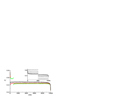
Figure 2: Density profiles for a $N=1000$ lattice with one slow site at $k=2$ (black), $10$ (dark grey, red online) and $82$ (light grey, green online) with $q=0.6$. Inset: Density profiles for $q=0.2$, $0.4$, $0.6$ and $0.8$ (from top to bottom on the left, and bottom to top on the right). The slow site sits at the center ($k=500$), and $N=1000$. In all cases, the profiles are discontinuous across the defect bond.

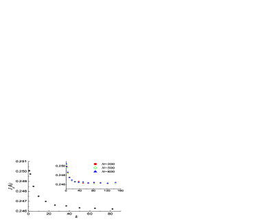
Figure 3: $J_{q}(k)$ as a function of the position $k$of the slow site for $q=0.6$ and $N=1000$. $J_{q}(k)$ approaches the limit 0.2463(5) as $k\rightarrow 500$. The inset shows that $J_{q}(k)$ is independent of $N$, within statistical fluctuations.

The “tails”, i.e., the deviations from the relatively slowly varying bulk values, are quite noticeable in the vicinity of both the slow site and the edges of the system. Though reminiscent of the profiles shown schematically in HadN , ours differ qualitatively, as a result of the loss of the $i\Leftrightarrow N-i-1$ symmetry ($k\neq N/2$), as well as $\alpha=\beta=1$ instead of $1/2$. Not surprisingly, there is no discernable relationship between the profiles of the two sublattices (except in the inset). More significantly, for our case the profiles (within each sublattice) are non-monotonic, a feature that necessarily contradicts mean-field predictions. Turning to the current, we see that, except for the smallest $q$’s, serious deviations from Eq. (2) emerge. Fig. 3, for $q=0.6$, shows that the current increases monotonically when the slow site is located closer and closer to the boundaries. Other choices of $q$ lead to similar behavior. Since particle-hole symmetry holds, $J_{q}(k)$ is symmetric under inversion, $k\rightarrow N+1-k$. To quantify the $k$-dependence, we define a relative change in the current,

$$\Delta_{1}(q)=\frac{J_{q}(1)-J_{q}(\infty)}{J_{q}(\infty)}$$ (4)

As illustrated by Fig. 4, the magnitude of this difference depends sensitively on $q$, reaching a maximum at $q=0.49$ where the relative current increase is about $2.5\%$. We refer to this phenomenon as the “edge effect”. Since the current through the left and the right sublattices is controlled by the bulk densities there, our findings immediately imply that these bulk densities, denoted by $\rho_{bulk}$, also shift with $k$. This feature is clearly displayed in Fig. 3.

Figure 4: $\Delta_{1}(q)$ plotted vs. $q$, for $N$=1000.

Returning to Fig. 3, we note that significant deviations from the limiting value, $J_{q}(\infty)$, are limited to a narrow window of $\delta\simeq 20$ sites near the boundaries. Thanks to charge-parity (CP) invariance, both entry and exit edges display identical behaviors, therefore we may restrict ourselves to, e.g., the region near the entrance. We believe that the origin of this length scale can be traced to the presence of exponential tails in the density profiles of the ordinary TASEP. For a homogeneous TASEP in the H phase, with entrance and exit rates $\alpha$ and $\beta$, the density decays exponentially into the bulk, as $\rho_{\ell}-\rho_{bulk}\sim\exp(-\ell/\xi)$. For $\alpha>1/2$, the decay length becomes independent of $\alpha$ and is given by Schutz

$$\xi(\beta)=-\frac{1}{\ln\left[4\beta(1-\beta)\right]}$$ (5)

In our case, we have $\alpha=1$, while $q_{eff}=q/(1+q)$ plays the role of $\beta$. Thus, for the $q=0.6$ case, we find $\xi(q_{eff})\simeq 15.5$. If the slow site is placed so close to the boundary that $k\lesssim\xi(q_{eff})$, we should certainly expect to see deviations from Eq. (2) , a formula underpinned by the assumption $k\gg 1$. In support of our conjecture, we note that first, the observed $\delta$ is consistent with $\xi(q_{eff})$, and second, that $\delta$, like $\xi(q_{eff})$, is at most weakly dependent on the system size (cf. the inset of Fig. 3). More detailed investigations are in progress, to settle this issue decisively Dong-un . In particular, if power laws such as the ones observed by HadN were to prevail, this picture would have to be revised.

According to the mean-field theory described in the former section, the presence of a defect with $q>1$ (a “fast site”), located at the center of the lattice, should have no noticeable effect on the current Kolo . Of course, it is not immediately apparent whether this statement remains true if the fast site is moved closer to the system boundaries. To explore whether such a an edge effect emerges, we consider the extreme case of $q=\infty$. Our simulation results confirms that the current does indeed remain unchanged. We find $J_{q}(k)=1/4+$ $O(1/N)$, consistent with the expected behavior of the M phase. In contrast to the current, the density profiles display a dramatic signature of the fast bond, as illustrated by Fig. 6.

Figure 5: Density profile for $q=\infty$, $k=500$ and $N$=1000.

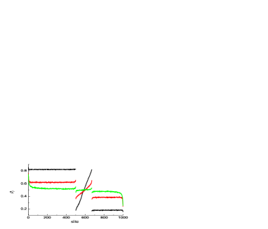
Figure 6: Density profiles for two slow sites, both with $q=0.2$ (black), $0.5$ (dark grey, red online), and $0.8$ (light grey, green online). The system size is $N=1000$, and the two slow sites are located at $k_{1}=500$, and $k_{2}=670$, resulting in $d=170$.

If we consider the edge effect as an interaction of the slow site with the lattice boundaries, the natural next step is to explore the interactions between two slow sites TomChou . In order to avoid edge effects, we place the two slow sites sufficiently far away from the boundaries and vary their separation.

Fig. 6 shows several typical density profiles. If $q$ is rather small (e.g., $0.2$), CL already noted the expected linear behavior in the central section, caused by the “wandering shock.” For larger $q$, however, the center profile begins to develop distinct tails near the two slow sites. Turning to the current, $J_{q}(d)$, we see from Fig. 8 that it is consistent with Eq. (3), for $d\gtrsim 50$, up to a finite-size correction of $O(1/N)$. In contrast, confirming the results of CL, we observe significant deviations from Eq. (3), when $d$ is decreased. We quantify the difference by defining

$$\Delta_{2}(q)=\frac{J_{q}(1)-J_{q}(\infty)}{J_{q}(\infty)}$$ (6)

where the arguments now refer to the distance between the two slow sites. In contrast to $\Delta_{1}$, we observe that $\Delta_{2}$ exhibits a sizable dependence on $q$, especially for small values of $q$. Indeed, as already noted by CL, one can show that, in the limit of $q\rightarrow 0$ the current decreases by a factor of 2. The data in Fig. 8 are clearly consistent with this conclusion. To sum up in words, two bottlenecks near each other have a dramatic effect on the current. Following CL, we may regard this phenomenon as an “interaction” between the two slow sites, inducing far more “resistance” when they are close than when they are well-separated.

Figure 7: $J_{q}(d)$ for $q=0.2$ and $N=1000$, as a function of $d$. One slow site is located at $k_{1}=500$, and $k_{2}$ is varied.

Figure 8: $\Delta_{2}(q)$ plotted vs. $q$, for $N$=1000. See also Fig. 5(c) in TomChou .

Two additional comments are in order. First, we return to one of the predictions of the mean-field theory, namely that a second slow site, spaced far apart from its partner, should have no further effect on the current. Our data indicate that the current for two slow sites, spaced far apart, is systematically lower than the current for a single slow site, but only by a very small amount (less than $1\%$). Second, we can again attempt to identify a length scale which controls how $J_{q}(d)$ approaches $J_{q}(\infty)$, as $d$ increases. Since the central section of the system displays a shock, it is natural to ask whether the intrinsic width of the shock sets this length scale. According to Janowsky ; JandL , this width covers only a few lattice spacings in the periodic TASEP with a single defect. Here, however, it appears that the shock broadens; preliminary data Dong-un indicate a width of about $40$ sites for $q=0.2$, which is not inconsistent with Fig. 8. Again, this behavior appears to be independent of the system size $N$. More work is needed to fully explore this intriguing characteristic.

IV Summary, Conclusions and Outlook

To summarize, we study an inhomogeneous open-boundary TASEP with one or two “slow” sites ($q<1)$. Our key findings are as follows: For a single slow site, there is an “edge effect”: moving the defect closer to the boundary enhances the current. The relative enhancement depends on $q$, but the effect is relatively small under all model conditions (at most $2.5\%$, for $q=0.49$). A single fast site, on the other hand, has no effect on the current, irrespective of its location. A much more significant effect, with clear biological implications, emerges in the case of two slow sites. This was already noted by CL, and we confirm their findings: As a function of the separation between the two sites, the current $J_{q}(d)$ decreases significantly, as the two sites approach each other. A quantitative measure of this effect is the fractional reduction: $\Delta_{2}(q)$. Its dependence on $q$ (Fig. 8) is nontrivial: In the $q\rightarrow 0$ limit, the current is reduced by as much as a factor of 2.

In order to gain a better understanding of these “interactions” between slow sites, and between slow sites and the system boundaries, we investigate particle (ribosome) density profiles. Every slow site displays a clear signature in the density profile, fully consistent with those in previous studies Kolo ; HadN . If a defect is located at site $k$, the profile is discontinuous between $k$ and $k+1$, and this discontinuity is surrounded by a “boundary layer”, or “tails”, where the densities deviate significantly from their bulk (asymptotic) values. In addition, the profiles display boundary layers near the system edges, as in the ordinary TASEP. When a defect is placed so close to a system edge or another defect that these boundary layers begin to overlap, the particle current develops a sensitivity to the defect-defect or defect-edge separation. In all other cases, the current is limited by the slowest codon in the system. In this sense, the slowest codon acts as a “gate keeper”.

The above findings are significant in the sense that these currents are directly linked to the protein production rate. Therefore, our results should be directly applicable to “designer genes”, repeating the same codon, except at one or two locations. If the defect codons are “fast”, i.e., associated with a highly abundant aa-tRNA, the production rate of the corresponding protein is insensitive to the presence of the defect codons, but the ribosome distribution on the mRNA will display a kink. In contrast, if the defect codons are “slow”, i.e., associated with rare aa-tRNAs, the protein production rate is significantly reduced. The magnitude of the reduction depends on the locations of the slow codons. A single slow codon near the beginning (or end) of the gene allows for a higher production rate than a single slow codon further away, and two slow codons placed next to one another generate a much more drastic reduction than two slow codons spaced far apart. Preliminary studies Dong-un indicate that our findings remain qualitatively correct even if the particles (ribosomes) cover more than just one site.

We can venture some even more wider-ranging predictions. Since several different aa-tRNA (anticodons) can be associated with the same amino acid, it is possible to produce the same protein from several different codon sequences which will have different production rates. Given a particular gene, we can obviously maximize the production rate of its associated protein by systematically replacing all slow codons with synonymous, faster ones. However, in many genes this requires a large number of substitutions which tends to be impracticable. Instead, our findings lead us to believe that we can pinpoint a small number (two or three) of selected substitutions (focusing on the slowest codons, or groups of several slow codons clustered together) which lead to nearly optimized production rates, with considerably less effort. Preliminary data for real codon sequences lend first support to this conjecture, and work is in progress to test these ideas more thoroughly in silicon and in vitro Dong-un .

- (1) C. MacDonald, J. Gibbs, and A. Pipkin, Biopolymers, 6, 1 (1968); C. MacDonald and J. Gibbs, Biopolymers, 7, 707 (1969).
- (2) B. Derrida, E. Domany, and D. Mukamel, J. Stat. Phys. 69, 667 (1992).
- (3) B. Derrida, M.R. Evans, V. Hakim, and V. Pasquier, J. Phys. A: Math. Gen. 26, 1493 (1993).
- (4) G.M. Schütz and E. Domany, J. Stat. Phys. 72, 277 (1993).
- (5) B. Derrida, Phys. Rep. 301, 65 (1998).
- (6) G.M. Schütz, in Phase Transition and Critical Phenomena edited by C. Domb and J.L. Lebowitz (Academic Press, San Diego, 2000).
- (7) J. Solomovici, T. Lesnik and C. Reiss, J. Theor. Biol, 185, 511 (1997).
- (8) C.M. Stenström, H. Jin, L.L. Major, W.P. Tate, and L.A. Isaksson, Gene 263, 273 (2001).
- (9) T. Chou and G. Lakatos, Phys. Rev. Lett. 93, 198101 (2004).
- (10) M. Robinson, R. Lilley, S. Little, J.S. Emtage, G. Yarranton, P. Stephens, A. Millican, M. Eaton, and G. Humphreys, Nucleic Acids Res. 12, 6663 (1984).
- (11) M.A. Sorensen, C.G. Kurland, and S. Pedersen, J. Mol. Biol. 207, 365 (1989).
- (12) B. Alberts, A. Johnson, J. Lewis, M. Raff, K. Roberts, and P. Walter, in Molecular biology of the cell, 4th ed. (Garland Science, New York, NY, 2002)
- (13) F. Neidhardt and H. Umbarger, in Escherichia coli and Salmonella, 2nd ed. edited by F.C. Neidhardt (ASM Press, Washington D.C., 1996).
- (14) R. Heinrich and T. Rapoport, J. Theo. Biol. 86, 279 (1980).
- (15) C. Kang and C. Cantor, J. Mol. Struct. 181, 241 (1985).
- (16) L.B. Shaw, R.K.P. Zia, and K.H. Lee, Phys. Rev. E 68, 021910 (2003).
- (17) J.J. Dong, B. Schmittmann, and R.K.P. Zia, to be published.
- (18) A. Kolomeisky, J. Phys. A: Math. Gen. 31, 1153 (1998).
- (19) S. Janowsky and J. Lebowitz, Phys. Rev. A 45, 618 (1992).
- (20) S. Janowsky and J. Lebowitz, J. Stat. Phys. 77, 35 (1994).
- (21) R.J. Harris and R.B. Stinchcombe, Phys. Rev. E 70, 016108 (2004).
- (22) M. Ha, J. Timonen, and M. den Nijs, Phys. Rev. E 68, 056122 (2003). For more details, see also M. Ha, PhD thesis, University of Washington, 2003.
- (23) L.B. Shaw, A.B. Kolomeisky and K.H. Lee, J. Phys. A: Math. Gen. 37, 2105 (2004).