Optimized parallel tempering simulations of proteins

Abstract

We apply a recently developed adaptive algorithm that systematically improves the efficiency of parallel tempering or replica exchange methods in the numerical simulation of small proteins. Feedback iterations allow us to identify an optimal set of temperatures/replicas which are found to concentrate at the bottlenecks of the simulations. A measure of convergence for the equilibration of the parallel tempering algorithm is discussed. We test our algorithm by simulating the 36-residue villin headpiece sub-domain HP-36 where we find a lowest-energy configuration with a root-mean-square-deviation of less than $4$ Å to the experimentally determined structure.

I Introduction

Understanding the folding of proteins from computer simulations is a longstanding but still elusive goal in computational biology. The difficulties stem from the fact that proteins are only marginal stable. At room temperature the free energy difference between the biologically active and unfolded states is only of order $\approx 10$ Kcal/mol. However, this small gap is due to cancelations of large energetic and entropic terms which poses two major challenges to numerical simulations. On the one hand, one has to find a universal model that captures this delicate balance. On the other hand, the competing interactions necessarily lead to a rugged energy landscape that makes the exhaustive sampling of low-temperature configurations a challenging computational task. In general, it has been hard to distinguish which of the two difficulties is the limiting factor in computational protein studies.

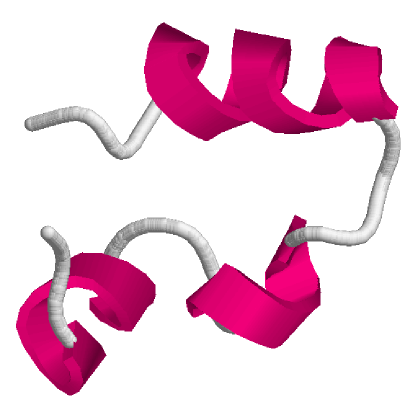
Figure 1: (color online) NMR-derived structure of the 36-residue peptide HP-36 as deposited in the Protein Data Bank (1vii).

In this paper we address the second challenge and apply a powerful sampling technique that allows to efficiently explore a complex energy landscape by systematically shifting computational resources towards the bottlenecks of a simulation OptimalEnsemble ; OptimalTempering , which are typically in the vicinity of free energy barriers. We test our algorithm by simulating the 36-residue villin headpiece sub-domain HP-36. This molecule has raised considerable interest in computational biology Freed ; Ripoli as it is one of the smallest proteins with well-defined secondary and tertiary structure McKnight:96 but at the same time with 596 atoms still accessible to simulations Duan:98 . Its structure which was resolved by NMR analysis and deposited in the Protein Data Bank (PDB code 1vii) is shown in Fig. 1.

Recent computationally intensive investigations have studied this protein using molecular dynamics Zagrovic:02 and parallel tempering Li:03 techniques. While the former study reports room temperature configurations that are within $<4.0$ Å to the native structure, these randomly sampled configurations could not be singled out from the misfolded structures in a rigorous way. The latter study Li:03 tries to identify the biologically active state as those configurations which minimize the energy functional of an implicit solvent model. However, despite considerable long simulation times low-energy configurations that resemble the experimentally determined one were found only with less than 20% frequency at T=250 K. These conformers differed still by root-mean-square-deviations (RMSD) of $\sim 4-6$Å  from the native structure and could also not be distinguished by their energies from that of the predominant misfolded structure. What leads to the discrepancy with the experiments? The authors of Ref. Li:03, argue that it is due to poor approximations of the simulated force field and especially the implicit solvent model. Indeed, configurations with an RMSD of $\approx 4$ Å  have been found later with high frequency in simulations with a modified energy function Hansmann:04 . However, the alterations of the implicit solvent model are ad hoc and not universal WH:05 , while the parameters of the original model were fitted against experimental data. On the other hand, the data of Ref. Li:03, could also indicate that despite large computational efforts the simulation has not thermalized and the correct equilibrium distribution of low-energy configurations not yet been found.

Deciding between the two alternatives in the above example is especially important as parallel tempering  Tempering (also known as replica exchange method) has recently become the simulation technique of choice in protein studies Hansmann:97 ; Hansmann:99 ; Hansmann:03 . The question can be re-formulated as how does one gauge the efficiency of a parallel tempering run and ensures that the sampling is sufficiently long to ensure thermal equilibration? The present paper describes a measure for this purpose and discusses a protocol that allows one to optimize the performance of parallel tempering runs by finding the best temperature distribution. Using the enhanced parallel tempering protocol we demonstrate that the simulation of Ref. Li:03, had indeed not thermalized. On the contrary, we now find a dominant lowest energy configuration that is within $<4.0$ Å to the native structure. This RMSD is comparable to the best ones found in previous molecular dynamics simulations Zagrovic:02 with a different search technique and energy function, but our approach requires only 1% of their computational resources.

II Algorithm Design

In parallel tempering Tempering simulations $N$ non-interacting copies, or “replicas”, of the protein are simultaneously simulated at a range of temperatures $\{T_{1},T_{2},\ldots,T_{N}\}$, e.g. by distributing the simulation over $N$ nodes of a parallel computer. After a fixed number of Monte Carlo sweeps (or a molecular dynamics run of a certain time) a sequence of swap moves, the exchange of two replicas at neighboring temperatures, $T_{i}$ and $T_{i+1}$, is suggested and accepted with a probability

$$p(E_{i},T_{i}\rightarrow E_{i+1},T_{i+1})=\min\left(1,\exp(-\Delta\beta\Delta E)\right)\;,$$ (1)

where $\Delta\beta=1/T_{i+1}-1/T_{i}$ is the difference between the inverse temperatures and $\Delta E=E_{i+1}-E_{i}$ is the difference in energy of the two replicas. For a given replica the swap moves induce a random walk in temperature space that allows the replica to wander from low temperatures, where barriers in a complex energy landscape lead to long relaxation times, to high temperatures, where equilibration is rapid, and back. The convergence of a parallel tempering run is given by the relaxation at lowest temperature and can be gauged by the frequency of statistically independent visits at this temperature. A lower bound for this number is the rate of round-trips $n_{rt}$ between the lowest and highest temperature, $T_{1}$ and $T_{N}$ respectively. An equivalent measure is the round-trip time $\tau_{1N}$, i.e. the average time it takes a replica to move from lowest temperature $T_{1}$ to the highest temperature $T_{N}$, and back. It is this non-local measure in temperature space that one has to minimize in order to optimize a parallel tempering simulation Dayal:04 ; OptimalEnsemble . Commonly, it is assumed that equilibration is fastest if the local acceptance rate of swaps is the same for all pairs of neighboring temperatures $T_{i}$ and $T_{i+1}$ Kofke:04 ; Predescu:04 ; Kone:05 ; Rathore:05 ; Predescu:05 . Recently, it has been shown that this assumption is misleading OptimalTempering . Here we review the algorithm outlined in Ref. OptimalTempering and apply it to systematically optimize the temperature set used in our simulations in such a way that for each replica the number of round-trips is maximized, and equilibration of the system at low temperatures thereby substantially improved.

We illustrate this approach by an example parallel tempering simulation of the 36-residue protein HP-36 in an all-atom representation. The intramolecular interactions are described by the ECEPP/2 force field ECEPP

$$E_{\text{ECEPP/2}} = E_{C}+E_{LJ}+E_{tor}$$ (2)

$$= \sum_{(i,j)}\frac{332q_{i}q_{j}}{\epsilon r_{ij}}+\sum_{(i,j)}\left(\frac{A_{ij}}{r_{ij}^{12}}-\frac{B_{ij}}{r_{ij}^{6}}\right)$$

$$+\sum_{l}U_{l}(1\pm\cos(n_{l}\xi_{l}))\;,$$

where $r_{ij}$ is the distance between the atoms $i$ and $j$, $\xi_{l}$ is the $l$-th torsion angle, and energies are measured in Kcal/mol. The protein-solvent interactions are approximated by a solvent accessible surface term

$$E_{solv}=\sum_{i}\sigma_{i}A_{i}\;.$$ (3)

Here $A_{i}$ is the solvent accessible surface area of the $i-th$ atom in a given configuration, and $\sigma_{i}$ a solvation parameter for the atom $i$. For the present investigation we use the parameter set OONS of Ref. OONS, . Our implementation is based on the software package SMMP (Simple Molecular Mechanics for Proteins) SMMP which allowed us to distribute the simultaneous simulation of $N=20$ replicas on a beowulf cluster with 2.2 GHz Opteron processors. The initial temperature distribution for these replicas is listed in Table 1. A sequence of swap moves between neighboring temperatures is attemped after each Monte Carlo sweep where a sweep consists of a series of Metropolis tests for each of the dihedral angles. Note that the implementation of the force field differs slightly from the one in Ref. Li:03, leading to (irrelevant) differences in the absolute energy values.

Our approach to optimize the simulated temperature set is inspired by a recently introduced adaptive broad-histogram algorithm OptimalEnsemble that maximizes the rate of round-trips in energy space by shifting additional weight toward the bottlenecks of the simulation and has been outlined in the context of classical spin models in Ref. OptimalTempering . The bottlenecks of the simulation are identified by measuring the local diffusivity of the simulated random walk. In the case of a parallel tempering run, where we simulate a random walk in temperature space, this quantity is calculated by adding a label “up” or “down” to the replica that indicates which of the two extremal temperatures, $T_{1}$ or $T_{N}$ respectively, the replica has visited most recently. The label of a replica changes only when the replica visits the opposite extremum. For instance, the label of a replica with label “up” remains unchanged if the replica comes back to the lowest temperature $T_{1}$, but changes to “down” upon its first visit to $T_{N}$. For each temperature point in the temperature set $\{T_{i}\}$ we record two histograms $n_{\rm up}(T_{i})$ and $n_{\rm down}(T_{i})$. Before attempting a sequence of swap moves we increment at temperature $T_{i}$ that of the two histograms which has the label of the respective replica currently at temperature $T_{i}$. If a replica has not yet visited neither of the two extremal temperatures, we increment neither of the histograms. For each temperature point this allows us to evaluate the average fraction of replicas which diffuse from the lowest to the highest temperature as

$$f(T)=\frac{n_{\rm up}(T)}{n_{\rm up}(T)+n_{\rm down}(T)}.$$ (4)

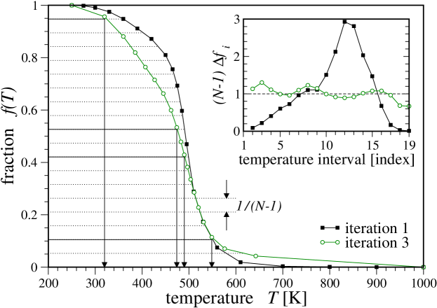
Figure 2: Fraction of replicas diffusing from the lowest, $T_{1}=250~{}$K, to the highest temperature $T_{N}=1000~{}$K in a parallel tempering simulation of HP-36. For the optimized temperature set (iteration 3), the temperature points are distributed in such a way that the fraction shows a nearly constant decay $\Delta f_{i}=f(T_{i})-f(T_{i+1})=1/(N-1)$ between adjacent temperature points, i.e. $\Delta f_{i}(N-1)\approx const$.

In Fig. 2 this fraction is plotted for our parallel tempering simulations of HP-36 with an initial temperature distribution as listed in Table 1.

The so-labelled replicas define a steady-state current current from $T_{1}$ to $T_{N}$ that is proportional to the round-trip rate $n_{rt}$ and therefore independent of temperature. To first order in the derivative this current is given by

$$j=D(T)\eta(T)\frac{df}{dT}\;,$$ (5)

where $D(T)$ is the local diffusivity at temperature $T$ and $\eta(T)$ is the probability distribution for a replica to reside at temperature $T$, where the temperature $T$ is now assumed to be a continuous variable (and not limited to the points of the current temperature set). For a given temperature set we approximate this probability distribution with a step-function $\eta(T)=C/\Delta T$, where $\Delta T=T_{i+1}-T_{i}$ is the length of the temperature interval around temperature $T_{i}<T<T_{i+1}$ in the current temperature set. The normalization constant $C$ is chosen as

$$\int_{T_{1}}^{T_{N}}\eta(T)dT=C\int_{T_{1}}^{T_{N}}\frac{dT}{\Delta T}=1\;.$$ (6)

Rearranging Eq. (5) gives a simple measure of the local diffusivity $D(T)$:

$$D(T)\sim\frac{\Delta T}{df/dT}\;,$$ (7)

where we have dropped the normalization $C$ and the constant current $j$.

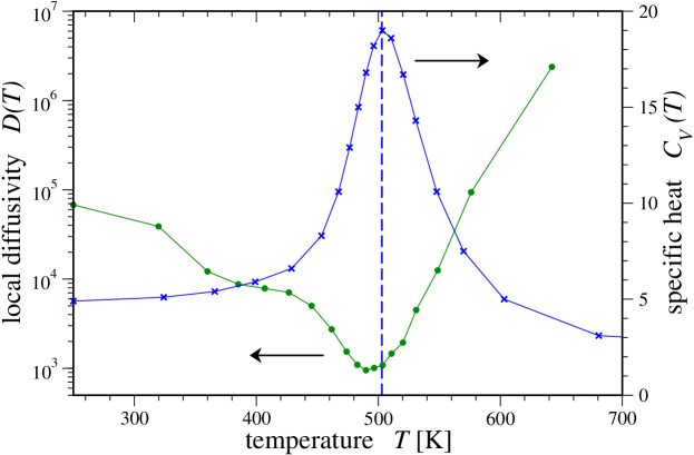
Figure 3: Local diffusivity $D(T)$ (left ordinate) for a random walk in temperature space preformed by a replica in a parallel tempering simulation of the chicken villin headpiece subdomain HP-36 using the ECEPP/2 force field and an implicit solvent. The diffusivity shows a strong modulation with temperature, note the logarithmic scale of the left ordinate. A pronounced minimum in the local diffusivity occurs slightly below the helix-coil transition around $T\approx 500$ K where the specific heat $C_{V}(T)$ (right ordinate) has a maximum (dashed line).

For the parallel tempering simulation of HP-36 this quantity is plotted in Fig. 3. The diffusivity shows a strong modulation along the simulated temperature range $250-1000$ K, note the logarithmic scale of the ordinate. A pronounced minimum occurs around $T\approx 490$ K where the diffusivity is suppressed by two orders of magnitude in comparison to the temperature range below 350 K and above 600 K. This minimum in the diffusivity points to a severe bottleneck for the random walk in temperature space: replicas can move back and forth in temperature rapidly below and above this bottleneck, but experience a dramatic slowdown as they approach and pass through the temperature range around 490 K. This behavior can be explained through a free energy barrier associated with a structural transition of the protein; the minimum in the local diffusivity is located slightly below the maximum of the specific heat at $T\approx 500$ K which is also plotted in Fig. 3. For HP-36 in the ECEPP/2 force-field it has been shown that the position of this peak separates a high-temperature phase with extended unordered configurations from a low-temperature region that is characterized by high helical content of the molecule Li:03 . Below this transition a shoulder in the measured local diffusivity points to a second bottleneck in the simulation for an extended range of temperatures $350~{}$K$~{}\leq T\leq 490~{}$K, possibly caused by competing low-energy configurations with high helical content. While the specific heat for this temperature range is slightly larger than in the high-temperature region above 600 K, there is no characteristic feature similar to the progression of the local diffusivity. The local diffusivity is thus a more sensitive measure to identify bottlenecks in a parallel tempering simulation and to locate the multiple temperature scales dominating the folding process of a protein for a given force field.

In order to speed up equilibration we want to maximize the rate of round-trips which each replica performs between the two extremal temperatures, or equivalently the diffusive current $j$, by varying the temperature set $\{T_{i}\}$ and thus the probability distribution $\eta(T)$, as discussed in Refs. OptimalEnsemble ; OptimalTempering . Rearranging and integrating Eq. (5) this goal is achieved by minimizing the integral

$$\frac{1}{j}=\int\left[\frac{1}{D(T)\eta(T)}+\lambda\eta(T)\right]dT\;,$$ (8)

where we have added a Lagrange multiplier $\lambda$ which ensures that $\eta(T)$ remains a normalized probability distribution. Varying the probability distribution $\eta(T)$ the integrand in Eq. (8) is minimized for

$$\eta^{\rm(opt)}(T)=\frac{C^{\prime}}{\Delta T^{\prime}}=C^{\prime}\sqrt{\frac{1}{\Delta T}\,\frac{df}{dT}}\sim\frac{1}{\sqrt{D(T)}}\;,$$ (9)

where the normalization $C^{\prime}$ is again chosen according to the normalization condition in Eq. (6). For the optimal temperature set the temperature points are thus rearranged in such a way that the probability distribution $\eta^{\rm(opt)}(T)$ becomes inversely proportional to the square root of the local diffusivity. Measuring the local diffusivity $D(T)$ for an initial temperature set, we can determine the optimized probability distribution $\eta^{\rm(opt)}(T)$ approximated as a step-function in the original temperature set. The optimized temperature set $\{T^{\prime}_{i}\}$ is then found by choosing the $n$-th temperature point $T^{\prime}_{n}$ such that

$$\int_{T^{\prime}_{1}}^{T^{\prime}_{n}}\eta^{\rm(opt)}(T)dT=n/N\;,$$ (10)

where $1<n<N$ and the two extremal temperatures $T^{\prime}_{1}=T_{1}$ and $T^{\prime}_{N}=T_{N}$ remain fixed. This feedback of the local diffusivity is then iterated for increasingly long simulation runs – in our simulations we double the number of swaps for subsequent feedback steps – until convergence of the optimized temperature set is found.

In our simulations we start with the arbitrary initial temperature set of Table 1 that similar to a geometric progression concentrates temperature points at low temperatures. Three feedback steps were performed, one after 100,000 MC sweeps, a second after further 200,000 sweeps, and a third one after additional 400,000 sweeps. The iterated temperature sets are plotted in Fig. 4 and also listed in Table 1. The feedback algorithm shifts computational resources towards the temperature of the helix-coil transition and temperature points in the optimized temperature sets concentrate around $T\approx 500$ K where the measured local diffusivity is suppressed, see Fig. 3. In the derivation of the feedback procedure we have assumed that the local diffusivity is to leading order independent from the temperature set. A posteriori we can verify this assumption by demonstrating that the optimized temperature set is independent of the initial temperature set. To this end, we perform a second series of feedback optimization steps starting from the temperature set of Ref. Li:03, . As illustrated in the lower half of Fig. 4 we indeed find that a very similar distribution is approached.

i

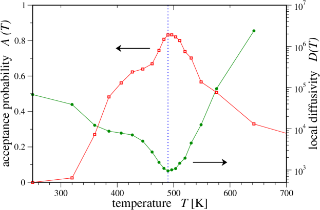
Figure 5: Acceptance probabilities (open squares) of replica swaps in a parallel tempering simulation of HP-36 using the optimized temperature set illustrated in Fig. 4. The dependence of the acceptance probabilities on the temperature closely reflects the shape of the measured local diffusivity (filled circles). In the vicinity of the helix-coil transition temperature $T\approx 500$ K where the local diffusivity is strongly suppressed the acceptance probabilities are highest due to the contraction of temperature points in the optimized temperature set. The dotted lines indicates the minimum in the local diffusivity.

For the optimized temperature set the acceptance probabilities of replica swaps show a strong temperature dependence as illustrated in Fig. 5. This is a consequence of the concentration of temperature points around $T\approx 500$ K in the optimized temperature set for HP-36. There the acceptance probabilities are found to be relatively high (around 80%) while in the temperature regions below 350 K and above 600 K where temperature points have been thinned out the acceptance probabilities drop below some 40%. The fact that for our optimized temperature set the acceptance probabilities vary with temperature contradicts various alternative approaches in the literature Kofke:04 ; Predescu:04 ; Kone:05 ; Rathore:05 ; Predescu:05 that aim at maximizing equilibration by choosing a temperature set where the acceptance probability of attempted swaps is independent of temperature.

III Simulation results –

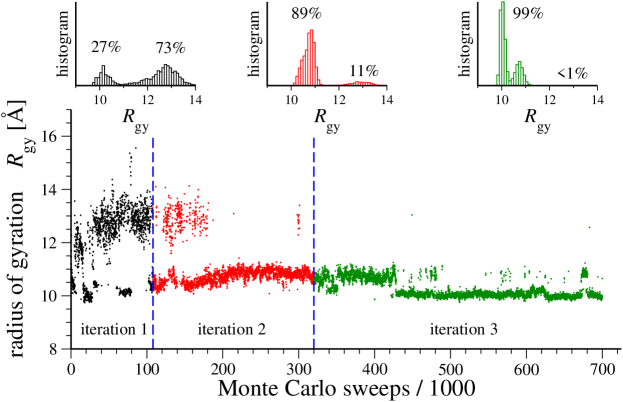
Figure 6: (color online) Radius of gyration of the lowest-energy configuration in a parallel tempering simulation of HP-36 versus the number of Monte Carlo sweeps. The dashed lines indicate when the temperature set used in the simulation was redefined as illustrated in the upper half of Fig. 4. The insets show histograms of the radius of gyration for the three simulation parts.

The feedback-iterations systematically optimize the temperature set which maximize the efficiency of parallel tempering simulations. We now turn to the results obtained for our simulations of HP-36 and discuss the effects of the temperature reweighting. Though the parallel tempering simulations allow to evaluate thermodynamic quantities over a range of temperatures, here we focus on the properties of the configurations at the lowest temperatures. In Fig. 6 the radius of gyration $R_{gy}$ which measures the compactness of a protein configuration is plotted for the lowest-energy configuration versus the number of Monte Carlo sweeps. For the initial iteration the radius of gyration varies in a broad range of $10-14$ Å. A histogram of $R_{gy}$ is plotted on top of the time series in Fig. 6 showing that two sets of configurations are found, one set with ”compact” configurations characterized by a radius of gyration in the range $10-11$ Å  and ”extended” configurations with a radius of gyration in the range $12-14$ Å. Averaging over some 100,000 MC sweeps in the first iteration we find that about 25% of the configurations are ”compact”, and a remaining 75% of ”extended” configurations. Previous simulations Li:03 with a total of 150,000 MC sweeps also reported the occurrence of these two sets of configurations. Similar to our case the ”extended” configurations dominated, and only a small fraction of 20% of the configurations were ”compact”. In the present study we continued the simulation after the first feedback step with an optimized temperature set for an additional 200,000 MC sweeps. The time series in Fig. 6 shows that as a consequence, the fraction of ”extended” configurations in the lowest-energy configurations is significantly reduced and some 90% of the sampled lowest-energy configuration have a radius of gyration smaller than 11 Å. This ratio increases further to 99% for the final iteration with 400,000 MC sweeps after the second feedback step. While in the previous study equilibration at low temperatures was determined by analyzing the time series for thermodynamic observables such as the potential energy and convergence was found after some 100,000 MC sweeps, the discrepancy to the results presented here cast serious doubt whether an overall simulation time of some 150,000 MC sweeps and a sub-optimal temperature set were sufficient to reach full equilibration. The long relaxation times in our example indicate that even with a sophisticated technique like parallel tempering the simulation times have to be considerably longer than commonly assumed. In order to assure equillibrisation at lowest temperature the number of round trip times should be at least $n_{rt}\approx 10$.

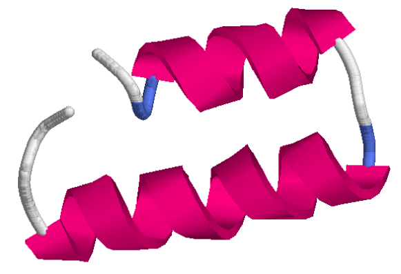
Figure 7: (color online) Lowest energy structure of HP-36 as obtained by an all-atom Monte Carlo simulation using the ECEPP/2 force field and an implicit solvent. The root-mean square deviation of this structure to the PDB structure shown in Fig. 1 is $r_{\text{RMSD}}=3.7$ Å.

To probe whether our simulations allow a structural prediction of the true ground state configuration we track the configuration with the overall lowest energy in the simulation and compare it to the Protein Data Bank structure of HP-36 (PDB code 1vii). The lowest-energy configuration obtained in our simulation is illustrated in Fig. 7. Despite the fact that in this structure the two N-terminal helices merged to one long helix (compromising residues 5 to 21) that tightly packs to the C-terminal helix, its RMSD to the PDB structure is only $r_{\text{RMSD}}=3.7$ Å. This value is substantially lower than in the structures with an RMSD of $r_{\text{RMSD}}\approx 5.8-6.0$ Å  previously obtained by molecular dynamics simlations Duan:98 , Monte Carlo simulations Li:03 ; Hansmann:04 and optimization techniques Hansmann:02 . A structure with comparable RMSD of $r_{\text{RMSD}}\approx 3.5$ Å  has been obtained by large-scale molecular dynamics simulations Zagrovic:02 . However, in those simulations the best-matching structure was found by comparing all sampled configurations along multiple trajectories to the PDB structure, while in our simulations the optimal structure is singled out as the one with the lowest energy. In addition, our simulations consumed only about 1% of the computing time resources (about 1,000 cpu years) used in Ref. Zagrovic:02, .

IV Conclusions –

In conclusion, we have applied a powerful feedback algorithm for the numerical simulation of proteins that allows to allocate computational resources in a parallel tempering simulation so that equilibration at all temperatures is considerably improved. By tracking the diffusion of replicas in temperature space we have identified the bottlenecks of a simulation, typically in the vicinity of the folding transition. Feeding back this information we obtain an optimal temperature set that concentrates temperature points at these bottlenecks. Our algorithm differs from previous approaches that aim at maximizing equilibration by considering the local acceptance probabilities of replica exchange moves. In contrast we find that for the optimal temperature set acceptance probabilities for such swap moves show a strong temperature dependence. Applying the optimized parallel tempering technique to the simulation of the 36-residue protein HP-36 we find a dominant low-energy configuration with less than 4 Å  root-mean square distance from the native structure within a fraction of the computing time consumed by high-performance molecular dynamics simulations.

We note, however, that the energy difference between our compact, lowest-energy configuration and the extended structure with lowest energy – which differs from the PDB structure by an RMSD of 8.0 Å– is only $\approx 10$ kcal/mol (for the minimized configurations). On the other hand, the energy of our lowest-energy configuration is 100 kcal/mol lower than that of the (minimized) PDB structure from which (despite the small RMSD) it still differs considerably. Hence, while our results appear to be closer to the experimental results than previous simulations they still demonstrate the limitations on protein simulations that are inherent in present energy functions. The extremely long relaxation times indicate the existence of spurious minima that should be absent in the folding funnel of fast folding proteins such as the villin headpiece. Unveiling these limitations in the energy functions and their underlying causes requires optimized simulation techniques such as the one applied in the present paper.

Acknowledgments – We thank A. Laio and B. Zagrovic for stimulating discussions, as well as D. A. Huse and H. G. Katzgraber for fruitful discussions on the technical aspects of this manuscript. S.T. acknowledges support by the Swiss National Science Foundation, U.H. by a research grant (CHE-9981874) of the National Science Foundation (USA).

Table 1: Temperature sets used in the parallel tempering simulation of HP-36. Applying the feedback algorithm temperature points in the optimized temperature sets (iterations 2,3 and 4) concentrate around the helix-coil transition around 500 K. The temperature sets are also illustrated in Fig. 4.

iteration	temperature set [$K$]
1	250	275	300	325	350	375	400	425	450	500	550	600	650	700	750	800	850	900	950	1000
2	250	295	326	349	371	395	424	446	464	482	499	514	528	543	559	577	595	628	693	1000
3	250	326	359	385	411	434	452	467	480	491	501	510	519	527	536	546	560	578	619	1000
4	250	314	358	381	402	423	444	461	474	484	494	502	511	519	529	540	554	576	670	1000

Figure 1: (color online) NMR-derived structure of the 36-residue peptide HP-36 as deposited in the Protein Data Bank (1vii).

Figure 2: Fraction of replicas diffusing from the lowest, $T_{1}=250~{}$K, to the highest temperature $T_{N}=1000~{}$K in a parallel tempering simulation of HP-36. For the optimized temperature set (iteration 3), the temperature points are distributed in such a way that the fraction shows a nearly constant decay $\Delta f_{i}=f(T_{i})-f(T_{i+1})=1/(N-1)$ between adjacent temperature points, i.e. $\Delta f_{i}(N-1)\approx const$.

Figure 3: Local diffusivity $D(T)$ (left ordinate) for a random walk in temperature space preformed by a replica in a parallel tempering simulation of the chicken villin headpiece subdomain HP-36 using the ECEPP/2 force field and an implicit solvent. The diffusivity shows a strong modulation with temperature, note the logarithmic scale of the left ordinate. A pronounced minimum in the local diffusivity occurs slightly below the helix-coil transition around $T\approx 500$ K where the specific heat $C_{V}(T)$ (right ordinate) has a maximum (dashed line).

Figure 4: (color online) Optimized temperature sets for a parallel tempering of HP-36 obtained by the feedback algorithm for two different initial temperature sets. Independent of the initial temperature set the optimized temperature sets converge to a temperature set that concentrates temperatures in the vicinity of the helix-coil transition temperature around $T\approx 500$ K (dashed line).

Figure 5: Acceptance probabilities (open squares) of replica swaps in a parallel tempering simulation of HP-36 using the optimized temperature set illustrated in Fig. 4. The dependence of the acceptance probabilities on the temperature closely reflects the shape of the measured local diffusivity (filled circles). In the vicinity of the helix-coil transition temperature $T\approx 500$ K where the local diffusivity is strongly suppressed the acceptance probabilities are highest due to the contraction of temperature points in the optimized temperature set. The dotted lines indicates the minimum in the local diffusivity.

Figure 6: (color online) Radius of gyration of the lowest-energy configuration in a parallel tempering simulation of HP-36 versus the number of Monte Carlo sweeps. The dashed lines indicate when the temperature set used in the simulation was redefined as illustrated in the upper half of Fig. 4. The insets show histograms of the radius of gyration for the three simulation parts.

Figure 7: (color online) Lowest energy structure of HP-36 as obtained by an all-atom Monte Carlo simulation using the ECEPP/2 force field and an implicit solvent. The root-mean square deviation of this structure to the PDB structure shown in Fig. 1 is $r_{\text{RMSD}}=3.7$ Å.

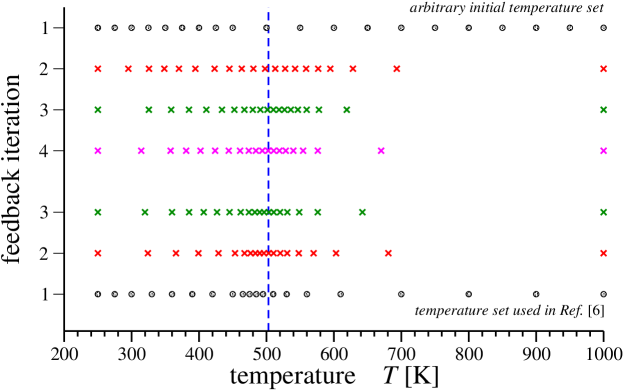
Figure 4: (color online) Optimized temperature sets for a parallel tempering of HP-36 obtained by the feedback algorithm for two different initial temperature sets. Independent of the initial temperature set the optimized temperature sets converge to a temperature set that concentrates temperatures in the vicinity of the helix-coil transition temperature around $T\approx 500$ K (dashed line).

References

- (1) S. Trebst, D.A. Huse, and M. Troyer, Phys. Rev. E 70, 046701 (2004).
- (2) H.G. Katzgraber, S. Trebst, D.A. Huse, and M. Troyer, cond-mat/0602085.
- (3) M.Y. Shen and K.F. Freed, Proteins 49 439 (2002).
- (4) D.R. Ripoli , J.A. Vila and H.A. Scheraga J. Mol. Biol. 339 915 (2004).
- (5) C.J. McKnight, D.S. Doehring, P.T. Matsudaria and P.S. Kim, J. Mol. Biol. 260, 126 (1996).
- (6) Y. Duan and P.A. Kollman, Science 282, 740 (1998).
- (7) B. Zagrovic et al., J. Mol. Biol. 323, 153i (2002).
- (8) C.-Y. Lin, C.-K. Hu and U.H.E. Hansmann Proteins: Structure, Functions and Genetics 52, 436 (2003).
- (9) U.H.E. Hansmann Phys. Rev. E 70, 012902 (2004).
- (10) W. Kwak and U.H.E. Hansmann, Phys. Rev. Lett. 95, 138102 (2005).
- (11) K. Hukushima and K. Nemoto, J. Phys. Soc. (Jpn.) 65, 1604 (1996); G.J. Geyer, Stat. Sci. 7, 437 (1992).
- (12) U.H.E. Hansmann, Chem. Phys. Lett. 281, 140 (1997).
- (13) U.H.E. Hansmann and Y. Okamoto, Curr. Opin. Struct. Biol. 9, 177 (1999).
- (14) U.H.E. Hansmann Comp. Sci. Eng. 5, 64 (2003).
- (15) P. Dayal et al. Phys. Rev. Letta. 92, 097201 (2004).
- (16) D.A. Kofke, J. Chem. Phys. 117, 6911 (2004).
- (17) C. Predescu, M. Predescu, and C. Ciabanu, J. Chem. Phys. 120, 4119 (2004).
- (18) A. Kone and D.A. Kofke, J. Chem. Phys. 122, 20610 (2005).
- (19) N. Rathore, M. Chopra, and J.J. de Pablo, J. Chem. Phys. 122, 024111 (2005).
- (20) C. Predescu, M. Predescu, and C. Ciabanu, J. Phys. Chem. B 109, 4189 (2005).
- (21) M.J. Sippl, G. Némethy, and H.A. Sheraga, J. Phys. Chem. 88, 6231 (1994).
- (22) T. Ooi, M. Obatake, G. Nemethy, H.A. Scheraga, Proc. Natl. Acad. Sci. USA 8, 3086 (1987).
- (23) F. Eisenmenger, U.H.E. Hansmann, Sh. Hayryan, C.-K. Hu, Comp. Phys. Comm. 138, 192 (2001).
- (24) U.H.E. Hansmann and L.T. Wille, Phys. Rev. Let. 88, 068105 (2002).
- (25) A. Schug, W. Wenzel, and U.H.E. Hansmann, J. Chem. Phys. 122, 194711 (2005).