STATISTICAL PROPERTIES OF THE INTERBEAT INTERVAL CASCADE IN HUMAN SUBJECTS

Abstract

Statistical properties of interbeat intervals cascade are evaluated by considering the joint probability distribution $P(\Delta x_{2},\tau_{2};\Delta x_{1},\tau_{1})$ for two interbeat increments $\Delta x_{1}$ and $\Delta x_{2}$ of different time scales $\tau_{1}$ and $\tau_{2}$. We present evidence that the conditional probability distribution $P(\Delta x_{2},\tau_{2}|\Delta x_{1},\tau_{1})$ may obey a Chapman-Kolmogorov equation. The corresponding Kramers-Moyal (KM) coefficients are evaluated. It is shown that while the first and second KM coefficients, i.e., the drift and diffusion coefficients, take on well-defined and significant values, the higher-order coefficients in the KM expansion are very small. As a result, the joint probability distributions of the increments in the interbeat intervals obey a Fokker-Planck equation. The method provides a novel technique for distinguishing the two classes of subjects in terms of the drift and diffusion coefficients, which behave differently for two classes of the subjects, namely, healthy subjects and those with congestive heart failure.

]

I Introduction

Cardiac interbeat intervals normally fluctuate in a complex manner.^1-6 Recent studies reveal that under normal conditions, beat-to-beat fluctuations in the heart rate may display extended correlations of the type typically exhibited by dynamical systems far from equilibrium. It has been argued,² for example, that the various stages of sleep may be characterized by long-range correlations of heart rates separated by a large number of beats. The interbeat fluctuations in the heart rates belong to a much broader class of many natural, as well as man-made, phenomena that are characterized by a degree of stochasticity. Turbulent flows, fluctuations in the stock market prices, seismic recordings, the internet traffic, and pressure fluctuations in packed-bed chemical reactors are example of time-dependent stochastic phenomena, while the surface roughness of many materials^7,8 are examples of such phenomena that are length scale-dependent.

The focus of the present paper is on the intriguing statistical properties of interbeat interval sequences, the analysis of which has attracted the attention of researchers from different disciplines.^9-15 Analysis of heartbeat fluctuations focused initially on short-time oscillations associated with breathing, blood pressure and neuroautonomic control.^16,17 Studies of longer heartbeat records, however, revealed $1/f-$like behavior.^18,19 Recent analysis of very long time series indicates that under healthy conditions, interbeat intervals may exhibit power-law anticorrelations,²⁰ follow universal scaling in their distributions,${21}$ and are characterized by a broad multifractal spectrum.²² Such scaling features change with the disease and advanced age.²³ The possible existence of scale-invariant properties in the seemingly noisy heartbeat fluctuations is may be attributed to highly complex, nonlinear mechanisms of physiological control,²⁴ as it is known that circadian rhythms are associated with periodic changes in key physiological processes.^25-33 In Figure 1 samples of interbeats fluctuations of healthy subjects and those with congestive heart failure (CHF) are shown.

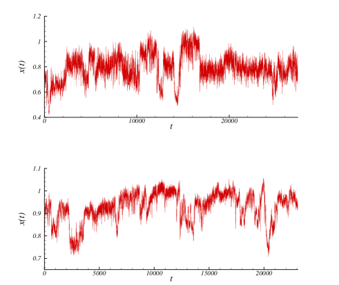
FIG. 1.: Time series of interbeat intervals $x(t)$ versus interval number $t$ for a typical person with congestive heart failure (bottom) and a healthy subject (top).

Recently, Friedrich and Peinke were able³⁴ to derive a Fokker-Planck (FP) equation for describing the evolution of the probability distribution function of stochastic properties of turbulent free jets, in terms of the relevant length scale. They pointed out that the conditional probability density of the increments of a stochastic field (for example, the increments in the velocity field in turbulent flow) satisfies the Chapman-Kolmogorov (CK) equation, even though the the velocity field itself contains long-range, nondecaying correlations. As is well-known, satisfying the CK equation is a necessary condition for any fluctuating data to be a Markovian process over the relevant length (or time) scales.³⁵ Hence, one has a way of analyzing stochastic phenomena in terms of the corresponding FP and CK equations. In this paper the method proposed by Friedrich and Peinke is used to compute the Kramers-Moyal (KM) coefficients for the increments of interbeat intervals fluctuatations, $\Delta x(\tau)=x(t+\tau)-x(t)$. Here, $\Delta x$ is the interbeat increments which, for all the samples, is defined as, $\Delta x\equiv\Delta x/\sigma_{\tau}$, where $\sigma_{\tau}$ is the standard deviations of the increments in the interbeats data. It is shown that the first and second KM coefficients representing, respectively, the drift and diffusion coefficients in the FP equation, have well-defined values, while the third- and fourth-order KM coefficients are small. Therefore, a FP evolution equation³⁵ is developed for the probability density function (PDF) $P(\Delta x,\tau)$ which, in turn, is used to gain information on changing the shape of PDF as a function of the time scale $\tau^{36}$ (see also Ref. [37] for another interesting and carefully-analyzed example of the application of the CK equation to stochastic phenomena).

The plan of this paper is as follows. In Section 2 we describe the Friedrich-Peinke method in terms of a KM expansion and the FP equation. We then apply the method in Section 3 to the analysis of the increments in the interbeat fluctuations.

II The Kramers-Moyal Expansion and Fokker-Planck Equation

A complete characterization of the statistical properties of the interbeat fluctuation requires evaluation of the joint PDFs, $P_{N}(\Delta x_{1},\tau_{1},\cdots,\Delta x_{N},\tau_{N})$, for an arbitrary $N$, the number of data points. If the phenomenon is a Markov process, an important simplification arises in that, the $N$-point joint PDF $P_{N}$ is generated by the product of the conditional probabilities $P(\Delta x_{i+1},\tau_{i+1}|\Delta x_{i},\tau_{i})$, for $i=1,\cdots,N-1$. Thus, as the first step of analyzing a stochastic time series, we check whether the increments in the data follow a Markov chain. As mentioned above, a necessary condition for a stochastic phenomenon to be a Markov process is that the CK equation,³⁴

$$P(\Delta x_{2},\tau_{2}|\Delta x_{1},\tau_{1})=$$ (1)

(2)

$$\int d(\Delta x_{3})\;P(\Delta x_{2},\tau_{2}|\Delta x_{3},\tau_{3})\;P(\Delta x_{3},\tau_{3}|\Delta x_{1},\tau_{1})\;,$$ (3)

should hold for any value of $\tau_{3}$, in the interval $\tau_{2}<\tau_{3}<\tau_{1}.^{35}$ Therefore, we check the validity of the CK equation for describing the data using many values of the $\Delta x_{1}$ triplets, by comparing the directly-evaluated conditional probability distributions $P(\Delta x_{2},\tau_{2}|\Delta x_{1},\tau_{1})$ with those calculated according to right-hand side of Eq. (1). In Fig. 2, the directly-computed PDF is compared with the one obtained from Eq. (1). Allowing for a statistical error of the order of the square root of the number of events in each bin, we find that the PDFs are statistically identical.

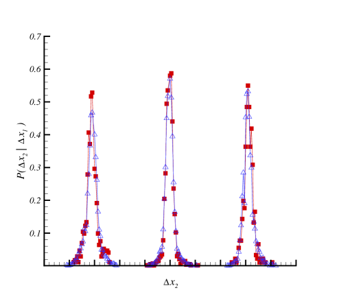
FIG. 2.: Test of Chapman-Kolmogorov equation for $\Delta x_{1}=-0.42$, $\Delta x_{1}=0$ and $\Delta x_{1}=0.42$. The solid and open symbols represent, respectively, the directly-evaluated PDF and the one obtained from Eq. (1). The PDFs are shifted in the horizontal directions for clarity. Values of $\Delta x$ are measured in units of the standard deviation of the increments. The time scales $\tau_{1}$, $\tau_{2}$ and $\tau_{3}$ are $10$, $30$, and $20$, respectively.

It is well-known that the CK equation yields an evolution equation for the distribution function $P(\Delta x,\tau)$ across the scales $\tau$. The CK equation, when formulated in differential form, yields a master equation, which takes on the form of a FP equation:³⁵

$$\frac{d}{d\tau}P(\Delta x,\tau)=$$ (4)

(5)

$$\left[-\frac{\partial}{\partial\Delta x}D^{(1)}(\Delta x,\tau)+\frac{\partial^{2}}{\partial\Delta x^{2}}D^{(2)}(\Delta x,\tau)\right]P(\Delta x,\tau)\;.$$ (6)

The drift and diffusion coefficients, $D^{(1)}(\Delta x,\tau)$ and $D^{(2)}(\Delta x,\tau)$, are estimated directly from the data and the moments $M^{(k)}$ of the conditional probability distributions:

$$D^{(k)}(\Delta x,\tau)=\frac{1}{k!}\lim_{\Delta\tau\to 0}M^{(k)}\;,$$ (7)

$$M^{(k)}=\frac{1}{\Delta\tau}\int d\Delta x^{\prime}\;(\Delta x^{\prime}-\Delta\tau)^{k}P(\Delta x^{\prime},\tau+\Delta\tau|\Delta x,\tau)\;.$$ (8)

The coefficients $D^{(k)}(\Delta x,\tau)$ are known as the Kramers-Moyal (KM) coefficients.

A Application to Analyzing Heartbeat Data

As an application of the method, we analyzed both daytime (12:00 pm to 18:00 pm) and nighttime (12:00 am to 6:00 am) heartbeat time series of healthy subjects, and the daytime records of patients with CHF. Our data base includes 10 healthy subjects (7 females and 3 males with ages between 20 and 50, and an average age of 34.3 years), and 12 subjects with CHF, with 3 females and 9 males with ages between 22 and 71, and an average age of 60.8 years). The resulting drift and diffusion coefficients, $D^{(1)}$ and $D^{(2)}$, are displayed in Figures 3 and 4. It turns out that the drift coefficient $D^{(1)}$ is a linear function of $\Delta x$, whereas the diffusivity $D^{(2)}$ is quadratic in $\Delta x$. Estimates of these coefficients are less accurate for large values of $\Delta x$ and, thus, the uncertainties increase. Using the data set for the healthy subjects we find that,

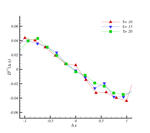
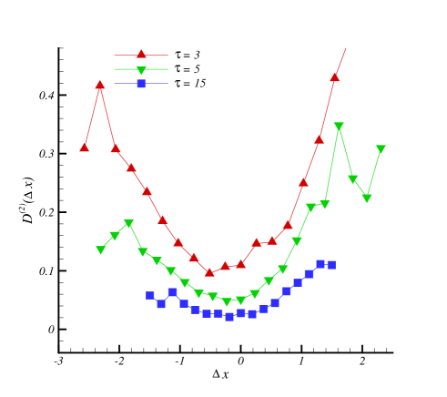
FIG. 3.: The drift and diffusion coefficients $D^{(1)}(\Delta x)$ and $D^{(2)}(\Delta x)$, estimated from Eq. (5) for a healthy subject, follow linear and quadratic behavior, respectively.

$$D^{(1)}(\Delta x,\tau)=-0.03\Delta x-0.0046\;,$$ (9)

(10)

$$D^{(2)}(\Delta x,\tau)=$$ (11)

(12)

$$\left(0.01+\frac{0.11}{\tau}\right)(\Delta x)^{2}+\left(0.057+\frac{0.287}{\tau}\right)\;,$$ (13)

whereas for the patients with CHF we obtain,

$$D^{(1)}(\Delta x,\tau)=-0.013\Delta x-0.0018\;,$$ (14)

(15)

$$D^{(2)}(\Delta x,\tau)=$$ (16)

(17)

$$\left(0.005+\frac{0.005}{\tau}\right)(\Delta x)^{2}+\left(0.013+\frac{0.066}{\tau}\right)\;.$$ (18)

We also computed the average of the coefficients $D^{(1)}$ and $D^{(2)}$ for the entire set of the healthy subjects, as well as those with CHF. According to the Pawula‘s theorem,^34,37 the KM expansion is truncated after the second term, provided that the fourth-order coefficient $D^{(4)}(\Delta x,\tau)$ vanishes. For the data that we analyze the coefficient $D^{(4)}$ is about $\frac{1}{10}D^{(2)}$ for the healthy subjects, and about $\frac{1}{20}D^{(2)}$ for those with CHF.

Equations (5) and (6) state that the drift coefficients for the healthy subjects and those with CHF have the same order of magnitude, whereas the diffusion coefficients for given $\tau$ and $\Delta x$ are different by about one order of magnitude. This points to a relatively simple way of distinguishing the two classes of the subjects. Moreover, the $\tau$-dependence of the diffusion coefficient for the healthy subjects is stronger than that of those with CHF (in the sense that the numerical coefficients of the $\tau^{-1}$ are larger for the healthy subjects). These are shown in Figures 3 and 4.

The strong $\tau-$dependence of the diffusion coefficient $D^{(2)}$ for the healthy subjects indicates that the nature of the PDF of their increments $\Delta x$ for given $\tau$, i.e., $P(\Delta x,\tau)$, is intermittent, and that its shape should change strongly with $\tau$. However, for the subjects with CHF the PDF is not so sensitive to the change of the time scale $\tau$, hence indicating that the increments’ fluctuations for the subjects with CHF is not intermittent. These results are completely compatible with the recent discoveries that the interbeat fluctuations for healthy subjects and those with CHF have fractal and multifractal properties, respectively.²²

III Summary

We have shown that the probability density of the interbeat interval increments satisfies a Fokker-Planck equation, which encodes the Markovian nature of the increments’ fluctuations. We have been able to compute reliably the first two Kramers-Moyal coefficients for the stochastic processes $\Delta x$ - the drift and diffusion coefficients in the FP representation - and, using the polynomial ansatz,³⁴ obtain simple expressions for them in terms of $\Delta x$ and the time scale $\tau$. We have shown that the drift and diffusion coefficients of the increments in the interbeat fluctuations of healthy subjects and patients with CHF have different behavior, when analyzed by the method we use in this paper. Hence, they help one to distinguish the two groups of the subjects. Moreover, one can obtain the form of the path probability functional of the increments in the interbeat intervals in the time scale, which naturally encodes the scale dependence of the probability density. This, in turn, provides a clear physical picture of the intermittent nature of interbeat intervals fluctuations.

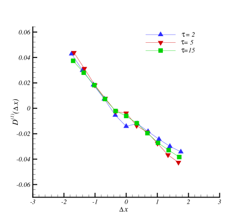
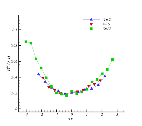
FIG. 4.: The drift and diffusion coefficients $D^{(1)}(\Delta x)$ and $D^{(2)}(\Delta x)$ are estimated from the Eq. (6) for typical patients with congestive heart failure, and follow linear and quadratic behavior, respectively.

Let us emphasize that the previous analysis^1-6 of the data that we consider in this paper indicated that there may be long-range correlations in the data which might be characterized by self-affine fractal distributions, such as the fractional Brownian motion or other types of stochastic processes that give rise to such correlations. In that method one distinguishes healthy subjects from those with CHF in terms of the type of the correlations that might exist in the data. For example, if the data follow a fractional Brownian motion, then the corresponding Hurst exponent $H$ is used to distinguish the two classes of the subjects, as $H<0.5$ ($>0.5$) indicates negative (positive) correlations in the data, while $H=0.5$ indicates that the increments in the data follow Brownian motion. The method proposed in the present paper is different from such analyses in that, the increments in the data are analyzed in terms of Markov processes. This is not in contradiction with the previous analyses. Our analysis does indicate the existence of correlations in the increments, but, as is well-known in the theory of Markov processes, such correlations, though extended, eventually decay. We distinguish the healthy subjects from those with CHF in terms of the differences between the drift and diffusion coefficients of the Fokker-Plank equation that we construct for the incremental data which, in our view, provides a clearer and more physical way of understanding the differences between the two groups of the subjects than the previous method.

REFERENCES

- [1] C.-K. Peng, J. Mietus, J.M. Hausdorrf, S. Havlin, H.E. Stanley, and A.L. Golbereger, Phys. Rev. Lett. 70, 1343 (1993).
- [2] A. Bunde, S. Havlin, J.W. Kantelhardt, T. Penzel, J.-H. Peter, and K. Voigt, Phys. Rev. Lett. 85, 3736 (2000).
- [3] P. Bernaola-Galvan, P.Ch. Ivanov, L.N. Amaral, and H.E. Stanley, Phys. Rev. Lett. 87, 168105 (2001).
- [4] V. Schulte-Frohlinde, Y. Ashkenanzy, P. Ch. Ivanov, L. Glass, A.L. Goldberger, and H.E. Stanley, Phys. Rev. Lett. 87, 068104 (2001).
- [5] Y. Ashkennanzy, P.Ch. Ivanov, S. Havlin, C.K. Peng, A.L. Goldberger, and H.E. Stanly, Phys. Rev. Lett. 86, 1900 (2001).
- [6] T. Kuusela, Phys. Rev. E 69, 031916 (2004).
- [7] S. Torquato, Random Hetrogenous Materials (Springer, New York, 2002).
- [8] M. Sahimi, Hetrogenous Materials, Volume II (Springer, New York, 2003).
- [9] M. Mackey and L. Glass, Science 197, 287 (1977).
- [10] M.M. Wolf, G.A. Varigos, D. Hunt, and J.G. Sloman, Med. J. Aust. 2, 52 (1978).
- [11] R.I. Kitney, D. Linkens, A.C. Selman, and A.A. McDonald, Automedica 4, 141 (1982).
- [12] Theory of Heart, edited by L. Glass, P. Hunter, and A. McCulloch (Springer, NewYork, 1991), p. 3.
- [13] J.B. Bassingthwaighte, L.S. Liebovitch, and B.J. West, Fractal Physiology (Oxford University Press, New York, 1994).
- [14] J. Kurths, A. Voss, P. Saparin, A. Witf, H.J. Kilner, and N. Wessel, Chaos 5, 88 (1995).
- [15] G. Sugihara, A. Allan, D. Sobel, and K.D. Allan, Proc. Natl. Acad. Sci. USA 93, 2608 (1996).
- [16] R.I. Kitney and O. Rompelman, The Study of Heart-Rate Variability (Oxford University Press, London, 1980).
- [17] S. Akselrod, D. Gordon, F.A. Ubel, D.C. Shannon, A.C. Barger, and R.J. Cohen, Science 213, 220 (1981).
- [18] M. Kobayashi and T. Musha, IEEE Trans. Biomed. Eng. 29, 456 (1982).
- [19] J.P. Saul, P. Albrecht, D. Berger, and R.J. Cohen, in Computers in Cardiology (IEEE Computer Society Press, Washington, 1987), p. 419.
- [20] C.-K. Peng, S. Havlin, H.E. Stanley, and A.L. Goldberger, Chaos 5, 82 (1995); R.G. Turcott and M.C. Teich, Ann. Biomed. Eng. 24, 269 (1996).
- [21] P. Ch. Ivanov, M.G. Rosenblum, C.-K. Peng, J. Mietus, S. Havlin, H.E. Stanley, and A.L. Goldberger, Nature 383, 323 (1996).
- [22] P.Ch. Ivanov, L.A.N. Amaral, A.L. Goldberger, S. Havlin, M.G. Rosenblum, Z.R. Struzik, and H.E. Stanley, Nature 399, 461 (1999).
- [23] L.A. Lipsitz, J. Mietus, G.B. Moody, and A.L. Goldberger, Circulation 81, 1803 (1990); D.T. Kaplan, et al., Biophys. J. 59, 945 (1991); N. Iyengar, et al., Am. J. Physiol. 271, R1078 (1996).
- [24] M.F. Shlesinger and B.J. West, in Random Fluctuations and Pattern Growth: Experiments and Theory, edited by H.E. Stanley and N. Ostrowsky (Kluwer Academic Publishers, Boston, 1988).
- [25] H. Moelgaard, K.E. Soerensen, and P. Bjerregaard, Am. J. Cardiol. 68, 777 (1991).
- [26] P.Ch. Ivanov, et al., Physica A 249, 587 (1998).
- [27] C.-K. Peng, S.V. Buldyrev, S. Havlin, M. Simons, H.E. Stanley, and A.L. Goldberger, Phys. Rev. E 49 1685 (1994); C.-K. Peng, J.M. Hausdorff, and A.L. Goldberger, in Nonlinear Dynamics, Self-Organization, and Biomedicine, edited by J. Walleczek (Cambridge University Press, Cambridge, 1999).
- [28] A.L. Goldberger, et al., Heart Am. J. 128, 202 (1994).
- [29] R.W. Peters, et al., J. Am. Coll. Cardiol. 23, 283 (1994); S. Behrens, et al., Am. J. Cardiol. 80, 45 (1997).
- [30] P.Ch. Ivanov, L.A.N. Amaral, A.L. Goldberger, and H.E. Stanley, Europhys. Lett. 43, 363 (1998).
- [31] P.Ch. Ivanov, A. Bunde, L.A.N. Amaral, S. Havlin, J. Fritsch-Yelle, R.M. Baevsky, H.E. Stanley, and A.L. Goldberger, Europhys. Lett. 48, 594 (1999).
- [32] R.M. Berne and M.N. Levy, Cardiovascular Physiology, 6th ed. (C.V. Mosby, St. Louis, 1996).
- [33] Heart Rate Variability, edited by M. Malik and A.J. Camm (Futura, Armonk, New York, 1995).
- [34] R. Friedrich and J. Peinke, Phys. Rev. Lett. 78, 863 (1997); R. Friedrich, J. Peinke, and C. Renner, ibid. 84, 5224 (2000); M. Ragwitz and H. Kantz, ibid. 87, 254501 (2001).
- [35] H. Risken, The Fokker-Planck Equation (Springer, Berlin, 1984).
- [36] J. Davoudi and M.R. Rahimi Tabar, Phys. Rev. Lett. 82, 1680 (1999).
- [37] G.R. Jafari, S.M. Fazlei, F. Ghasemi, S.M. Vaez Allaei, M.R. Rahimi Tabar, A. Iraji Zad, and G. Kavei, Phys. Rev. Lett. 91, 226101 (2003).