Computation of protein geometry and its applications: Packing and function prediction

6.1 Introduction

Three-dimensional atomic structures of protein molecules provide rich information for understanding how these working molecules of a cell carry out their biological functions. With the amount of solved protein structures rapidly accumulating, computation of geometric properties of protein structure becomes an indispensable component in studies of modern biochemistry and molecular biology. Before we discuss methods for computing the geometry of protein molecules, we first briefly describe how protein structures are obtained experimentally.

There are primarily three experimental techniques for obtaining protein structures: X-ray crystallography, solution nuclear magnetic resonance (NMR), and recently freeze-sample electron microscopy (cryo-EM). In X-ray crystallography, the diffraction patterns of X-ray irradiation of a high quality crystal of the protein molecule are measured. Since the diffraction is due to the scattering of X-ray by the electrons of the molecules in the crystal, the position, the intensity, and the phase of each recorded diffraction spot provide information for the reconstruction of an electron density map of atoms in the protein molecule. Based on independent information of the amino acid sequence, a model of the protein conformation is then derived by fitting model conformations of residues to the electron density map. An iterative process called refinement is then applied to improve the quality of the fit of the electron density map. The final model of the protein conformation consists of the coordinates of each of the non-hydrogen atoms [1].

The solution NMR technique for solving protein structure is based on measuring the tumbling and vibrating motion of the molecule in solution. By assessing the chemical shifts of atomic nuclei with spins due to interactions with other atoms in the vicinity, a set of estimated distances between specific pairs of atoms can be derived from NOSEY spectra. When a large number of such distances are obtained, one can derive a set of conformations of the protein molecule, each is consistent with all of the distance constraints [2]. Although determining conformations from either X-ray diffraction patterns or NMR spectra is equivalent to solving an ill-posed inverse problem, technique such as Bayesian Markov chain Monte Carlo with parallel tempering has been shown to be effective in obtaining protein structures from NMR spectra [3]. The cryo-EM technique for obtaining protein structure is described in more details in Chapter 11.

6.2 Theory and Model

6.2.1 The idealized ball model

The shape of a protein molecule is complex. The chemical properties of atoms in a molecule are determined by their electron charge distribution. It is this distribution that generates the scattering patterns of the X-ray diffraction. Chemical bonds between atoms lead to transfer of electronic charges from one atom to another, and the resulting isosurfaces of the electron density distribution depend not only on the location of individual nuclei but also on interactions between atoms. This results in an overall complicated isosurface of electron density [4].

The geometric model of macromolecule amenable to convenient computation is an idealized model, where the shapes of atoms are approximated by three-dimensional balls. The shape of a protein or a DNA molecule consisting of many atoms is then the space-filling shape taken by a set of atom balls. This model is often called the interlocking hard-sphere model, the fused ball model, the space filling model [5, 6, 7, 8], or the union of ball model [9]. In this model, details in the distribution of electron density, e.g., the differences between regions of covalent bonds and non-covalent bonds, are ignored. This idealization is quite reasonable, as it reflects the fact that the electron density reaches maximum at a nucleus, and its magnitude decays almost spherically away from the point of the nucleus. Despite possible inaccuracy, this idealized model has found wide acceptance, because it enables quantitative measurement of important geometric properties (such as area and volume) of molecules. Insights gained from these measurements correlate well with experimental observations [5, 10, 8, 11, 12, 13].

In this idealization, the shape of each atom is that of a ball, and its size parameter is the ball radius. There are many possible choices for the parameter set of atomic radii [14, 15]. Frequently, atomic radii are assigned the values of their van der Waals radii [16]. Among all these atoms, hydrogen atom has the smallest mass, and has a much smaller radius than those of other atoms. For simplification, the model of united atom is often employed to approximate the union of a heavy atom and the hydrogen atoms connected by a covalent bond. In this case, the radius of the heavy atom is increased to approximate the size of the union of the two atoms. This practice significantly reduces the total number of atom balls in the molecule. However, this approach has been questioned for possible inadequacy [17].

The mathematical model of this idealized model is that of the union of balls [9]. For a molecule $M$ of $n$ atoms, the $i$-th atom is modeled as a ball $b_{i}$, whose center is located at ${\mbox{\boldmath$z$}}_{i}\in{{\mathbb{R}}}^{3}$, and the radius of this ball is $r_{i}\in{{\mathbb{R}}}$, namely, we have $b_{i}\equiv\{{\mbox{\boldmath$x$}}|{\mbox{\boldmath$x$}}\in{{\mathbb{R}}}^{3},||{\mbox{\boldmath$x$}}-{\mbox{\boldmath$z$}}_{i}||\leq r_{i}\}$ parameterized by $({\mbox{\boldmath$z$}}_{i},r_{i})$. The molecule $M$ is formed by the union of a finite number $n$ of such balls defining the set $\cal B$:

$$M=\bigcup{\cal B}=\bigcup_{i=1}^{n}\{b_{i}\}.$$

It creates a space-filling body corresponding to the union of the excluded volumes $\operatorname{vol}(\bigcup_{i=1}^{n}b_{i})$ [9]. When the atoms are assigned the van der Waals radii, the boundary surface $\partial\bigcup{\cal B}$ of the union of balls is called the van der Waals surface.

6.2.2 Surface models: Lee-Richards and Connolly’s surfaces

Protein folds into native three-dimensional shape to carry out its biological functional roles. The interactions of a protein molecule with other molecules (such as ligand, substrate, or other protein) determine its functional roles. Such interactions occur physically on the surfaces of the protein molecule.

The importance of protein surface was recognized very early on. Lee and Richards developed the widely used solvent accessible surface (SA) model, which is also often called the Lee-Richards surface model [5]. Intuitively, this surface is obtained by rolling a ball of radius $r_{s}$ everywhere along the van der Waals surface of the molecule. The center of the solvent ball will then sweep out the solvent accessible surface. Equivalently, the solvent accessible surface can be viewed as the boundary surface $\partial\bigcup{\cal B}_{r_{s}}$ of the union of a set of inflated balls ${\cal B}_{r_{s}}$, where each ball takes the position of an atom, but with an inflated radius $r_{i}+r_{s}$ (Fig. 6.1a).

The solvent accessible surface in general has many sharp crevices and sharp corners. In hope of obtaining a smoother surface, one can take the surface swept out by the front instead of the center of the solvent ball. This surface is the molecular surface (MS model), which is often called the Connolly’s surface after Michael Connolly who developed the first algorithm for computing molecular surface [11]. Both solvent accessible surface and molecular surface are formed by elementary pieces of simpler shape.

Elementary pieces. For the solvent accessible surface model, the boundary surface of a molecule consists of three types of elements: the convex spherical surface pieces, arcs or curved line segments (possibly a full circle) formed by two intersecting spheres, and a vertex that is the intersection point of three atom spheres. The whole boundary surface of the molecules can be thought of as a surface formed by stitching these elements together.

Figure 6.1: Geometric models of protein surfaces. (a) The solvent accessible surface (SA surface) is shown in the front. The van der Waals surface (beneath the SA surface) can be regarded as a shrunken version of the SA surface by reducing all atomic radii uniformly by the amount of the radius of the solvent probe $r_{s}=1.4$Å. The elementary pieces of the solvent accessible surface are the three convex spherical surface pieces, the three arcs, and the vertex where the three arcs meet. (b) The molecular surface (MS, beneath the SA surface) also has three types of elementary pieces: the convex spheric pieces, which are shrunken version of the corresponding pieces in the solvent accessible surface, the concave toroidal pieces, and concave spheric surface. The latter two are also called the re-entrant surface. (c) The toroidal surface pieces in the molecular surface, correspond to the arcs in the solvent accessible surface, and the concave spheric surface to the vertex. The set of elements in one surface can be continuously deformed to the set of elements in the other surface.

Similarly, the molecular surface swept out by the front of the solvent ball can also be thought of as being formed by elementary surface pieces. In this case, they are the convex spherical surface pieces, the toroidal surface pieces, and the concave or inverse spherical surface pieces (Fig. 6.1b) . The latter two types of surface pieces are often called the “re-entrant surfaces” [11, 8].

The surface elements of the solvent accessible surface and the molecular surface are closely related. Imagine a process where atom balls are shrunk or expanded. The vertices in solvent accessible surface becomes the concave spherical surface pieces, the arcs becomes the toroidal surfaces, and the convex surface pieces become smaller convex surface pieces (Fig. 6.1c). Because of this mapping, these two type of surfaces are combinatorically equivalent and have similar topological properties, i.e., they are homotopy equivalent.

However, the SA surface and the MS surface differ in their metric measurement. In concave regions of a molecule, often the front of the solvent ball can sweep out a larger volume than the center of the solvent ball. A void of size close to zero in solvent accessible surface model will correspond to a void of the size of a solvent ball ($4\pi r_{s}^{3}/3$). It is therefore important to distinguish these two types of measurement when interpreting the results of volume calculations of protein molecules. The intrinsic structures of these fundamental elementary pieces are closely related to several geometric constructs we describe below.

6.2.3 Geometric constructs

Figure 6.2: Geometry of a simplified two dimensional model molecule, to illustrate the geometric constructs and the procedure mapping the Voronoi diagram to the Delaunay triangulation. (a) The molecule formed by the union of atom disks of uniform size. Voronoi diagram is in dashed lines. (b) The shape enclosed by the boundary polygon is the convex hull. It is tessellated by the Delaunay triangulation. (c) The alpha shape of the molecule is formed by removing those Delaunay edges and triangles whose corresponding Voronoi edges and Voronoi vertices do not intersect with the body of the molecule. A molecular void is represented in the alpha shape by two empty triangles.

Voronoi diagram. Voronoi diagram (Fig 6.2a), also known as Voronoi tessellation, is a geometric construct that has been used for analyzing protein packing in the early days of protein crystallography [6, 18, 19]. For two dimensional Voronoi diagram, we consider the following analogy. Imagine a vast forset containing a number of fire observation towers. Each fire ranger is responsible for putting out any fire closer to his/her tower than to any other tower. The set of all trees for which a ranger is responsible constitutes the Voronoi cell associated with his/her tower, and the map of ranger responsibilities, with towers and boundaries marked, constitutes the Voronoi diagram.

We formalize this for three dimensional space. Consider the point set $S$ of atom centers in three dimensional space ${{\mathbb{R}}}^{3}$. The Voronoi region or Voronoi cell $V_{i}$ of an atom $b_{i}$ with atom center ${\mbox{\boldmath$z$}}_{i}\in{{\mathbb{R}}}^{3}$ is the set of all points that are at least as close to ${\mbox{\boldmath$z$}}_{i}$ than to any other atom centers in ${\cal S}$:

$$V_{i}=\{{\mbox{\boldmath$x$}}\in{{\mathbb{R}}}^{3}|||{\mbox{\boldmath$x$}}-{\mbox{\boldmath$z$}}_{i}||\leq||{\mbox{\boldmath$x$}}-{\mbox{\boldmath$z$}}_{j}||,{\mbox{\boldmath$z$}}_{j}\in{\cal S}\}.$$ (6.1)

We can have an alternative view of the Voronoi cell of an atom $b_{i}$. Considering the distance relationship of atom center ${\mbox{\boldmath$z$}}_{i}$ with the atom center ${\mbox{\boldmath$z$}}_{k}$ of another atom $b_{k}$. The plane bisecting the line segment connecting points ${\mbox{\boldmath$z$}}_{i}$ and ${\mbox{\boldmath$z$}}_{k}$ divides the full ${{\mathbb{R}}}^{3}$ space into two half spaces, where points in one half space is closer to ${\mbox{\boldmath$z$}}_{i}$ than to ${\mbox{\boldmath$z$}}_{k}$, and points in the other allspice is closer to ${\mbox{\boldmath$z$}}_{k}$ than to ${\mbox{\boldmath$z$}}_{i}$. If we repeat this process and take ${\mbox{\boldmath$z$}}_{k}$ in turn from the set of all atom centers other than ${\mbox{\boldmath$z$}}_{i}$, we will have a number of halfspaces where points are closer to ${\mbox{\boldmath$z$}}_{i}$ than to each of the atom center ${\mbox{\boldmath$z$}}_{k}$. The Voronoi region $V_{i}$ is then the common intersections of these half spaces, which is convex. When we consider atoms of different radii, we replace the Euclidean distance $||{\mbox{\boldmath$x$}}-{\mbox{\boldmath$z$}}_{i}||$ with the power distance defined as: $\pi_{i}({\mbox{\boldmath$x$}})\equiv||{\mbox{\boldmath$x$}}-{\mbox{\boldmath$z$}}_{i}||^{2}-r_{i}^{2}$.

Delaunay tetrahedrization. Delaunay triangulation in ${{\mathbb{R}}}^{2}$ or Delaunay tetrahedrization in ${{\mathbb{R}}}^{3}$ is a geometric construct that is closely related to the Voronoi diagram (Fig 6.2b). In general, it uniquely tessellates or tile up the space of the convex hull of the atom centers in ${{\mathbb{R}}}^{3}$ with tetrahedra. Convex hull for a point set is the smallest convex body that contains the point set . The Delaunay tetrahedrization of a molecule can be obtained from the Voronoi diagram. Consider that the Delaunay tetrahedrization is formed by gluing four types of primitive elements together: vertices, edges, triangles, and tetrahedra. Here vertices are just the atom centers. We obtain a Delaunay edge by connecting atom centers ${\mbox{\boldmath$z$}}_{i}$ and ${\mbox{\boldmath$z$}}_{j}$ if and only if the Voronoi regions $V_{i}$ and $V_{j}$ have a common intersection, which is a planar piece that may be either bounded or extend to infinity. We obtain a Delaunay triangle connecting atom centers ${\mbox{\boldmath$z$}}_{i}$, ${\mbox{\boldmath$z$}}_{j}$, and ${\mbox{\boldmath$z$}}_{k}$ if the common intersection of Voronoi regions $V_{i},V_{j}$ and $V_{k}$ exists, which is either a line segment, or a half-line, or a line in the Voronoi diagram. We obtain a Delaunay tetrahedra connecting atom centers ${\mbox{\boldmath$z$}}_{i},{\mbox{\boldmath$z$}}_{j},{\mbox{\boldmath$z$}}_{k}$ and ${\mbox{\boldmath$z$}}_{l}$ if and only if the Voronoi regions $V_{i},V_{j},V_{k}$ and $V_{l}$ intersect at a point.

6.2.4 Topological structures

Delaunay complex. The structures in both Voronoi diagram and Delaunay tetrahedrization are better described with concepts from algebraic topology. We focus on the intersection relationship in the Voronoi diagram and introduce concepts formalizing the primitive elements. In ${{\mathbb{R}}}^{3}$, between two to four Voronoi regions may have common intersections. We use simplices of various dimensions to record these intersection or overlap relationships. We have vertices $\sigma_{0}$ as 0-simplices, edges $\sigma_{1}$ as 1-simplices, triangles $\sigma_{2}$ as 2-simplices, and tetrahedra $\sigma_{3}$ as 3-simplices. Each of the Voronoi plane, Voronoi edge, and Voronoi vertices corresponds to a 1-simplex (Delaunay edge), 2-simplex (Delaunay triangle), and 3-simplex (Delaunay tetrahedron), respectively. If we use 0-simplices to represent the Voronoi cells, and add them to the simplices induced by the intersection relationship, we can think of the Delaunay tetrahedrization as the structure obtained by “glueing” these simplices properly together. Formally, these simplices form a simplicial complex ${\cal K}$:

$${\cal K}=\{\sigma_{|I|-1}|\bigcap_{i\in I}V_{i}\neq\emptyset\},$$ (6.2)

where $I$ is an index set for the vertices representing atoms whose Voronoi cells overlap, and $|I|-1$ is the dimension of the simplex.

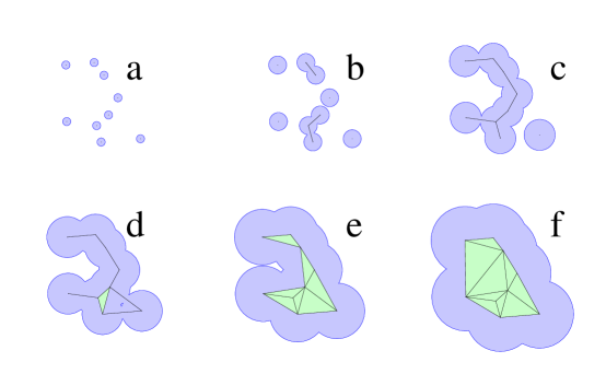
Figure 6.3: The family of alpha shapes or dual simplicial complexes for a two-dimensional toy molecule. (a) We collect simplices from the Delaunay triangulation as atoms grow by increasing the $\alpha$ value. At the beginning as $\alpha$ grows from $-\infty$, atoms are in isolation and we only have vertices in the alpha shape. (b) and (c) When $\alpha$ is increased such that some atom pairs start to intersect, we collect the corresponding Delaunay edges. (d) When three atoms intersect as $\alpha$ increases, we collect the corresponding Delaunay triangles. When $\alpha=0$, the collection of vertices, edges, and triangles form the dual simplicial complex ${\cal K}_{0}$, which reflecting the topological structure of the protein molecule. (e) More edges and triangles from the Delaunay triangulation are now collected as atoms continue to grow. (d) Finally, all vertices, edges, and triangles are now collected as atoms are grown to large enough size. We get back the full original Delaunay complex.

Alpha shape and protein surfaces. Imagine we can turn a knob to increase or decrease the size of all atoms simultaneously. We can then have a model of growing balls and obtain further information from the Delaunay complex about the shape of a protein structure. Formally, we use a parameter $\alpha\in{{\mathbb{R}}}$ to control the size of the atom balls. For an atom ball $b_{i}$ of radius $r_{i}$, we modified its radius $r_{i}$ at a particular $\alpha$ value to $r_{i}(\alpha)=(r_{i}^{2}+\alpha)^{1/2}$. When $-r_{i}<\alpha<0$, the size of an atom is shrunk. The atom could even disappear if $\alpha<0$ and $|\alpha|>r_{i}$. We start to collect the simplices at different $\alpha$ value as we increase $\alpha$ from $-\infty$ to $+\infty$ (see Fig 6.3 for a two-dimensional example). At the beginning, we only have vertices. When $\alpha$ is increased such that two atoms are close enough to intersect, we collect the corresponding Delaunay edge that connects these two atom centers. When three atoms intersect, we collect the corresponding Delaunay triangle spanning these three atom centers. When four atoms intersect, we collect the corresponding Delaunay tetrahedron. At any specific $\alpha$ value, we have a dual simplicial complex or alpha complex ${\cal K}_{\alpha}$ formed by the collected simplices. If all atoms take the incremented radius of $r_{i}+r_{s}$ and $\alpha=0$, we have the dual simplicial complex ${\cal K}_{0}$ of the protein molecule. When $\alpha$ is sufficiently large, we have collected all simplices and we get the full Delaunay complex. This series of simplicial complexes at different $\alpha$ value form a family of shapes (Fig 6.3), called alpha shapes, each faithfully represents the geometric and topological property of the protein molecule at a particular resolution parametrized by the $\alpha$ value.

An equivalent way to obtain the alpha shape at $\alpha=0$ is to take a subset of the simplices, with the requirement that the corresponding intersections of Voronoi cells must overlap with the body of the union of the balls. We obtain the dual complex or alpha shape ${\cal K}_{0}$ of the molecule at $\alpha=0$ (Fig 6.2c):

$${\cal K}_{0}=\{\sigma_{|I|-1}|\bigcap_{i\in I}V_{i}\cap\bigcup{\cal B}\neq\emptyset\}.$$ (6.3)

Alpha shape provides a guide map for computing geometric properties of the structures of biomolecules. Take the molecular surface as an example, the re-entrant surfaces are formed by the concave spherical patch and the toroidal surface. These can be mapped from the boundary triangles and boundary edges of the alpha shape, respectively [20]. Recall that a triangle in the Delaunay tetrahedrization corresponds to the intersection of three Voronoi regions, i.e., a Voronoi edge. For a triangle on the boundary of the alpha shape, the corresponding Voronoi edge intersects with the body of the union of balls by definition. In this case, it intersects with the solvent accessible surface at the common intersecting vertex when the three atoms overlap. This vertex corresponds to a concave spherical surface patch in the molecular surface. For an edge on the boundary of the alpha shape, the corresponding Voronoi plane coincides with the intersecting plane when two atoms meet, which intersect with the surface of the union of balls on an arc. This line segment corresponds to a toroidal surface patch. The remaining part of the surface are convex pieces, which correspond to the vertices, namely, the atoms on the boundary of the alpha shape.

The numbers of toroidal pieces and concave spherical pieces are exactly the numbers of boundary edges and boundary triangles in the alpha shape, respectively. Because of the restriction of bond length and the excluded volume effects, the number of edges and triangles in molecules are roughly in the order of ${\cal O}(n)$ [21].

6.2.5 Metric measurement

We have described the relationship between the simplices and the surface elements of the molecule. Based on this type of relationship, we can compute efficiently size properties of the molecule. We take the problem of volume computation as an example.

Consider a grossly incorrect way to compute the volume of a protein molecule using the solvent accessible surface model. We could define that the volume of the molecule is the summation of the volumes of individual atoms, whose radii are inflated to account for solvent probe. By doing so we would have significantly inflated the value of the true volume, because we neglected to consider volume overlaps. We can explicitly correct this by following the inclusion-exclusion formula: when two atoms overlap, we subtract the overlap; when three atoms overlap, we first subtract the pair overlaps, we then add back the triple overlap, etc. This continues when there are four, five, or more atoms intersecting. At the combinatorial level, the principle of inclusion-exclusion is related to the Gauss-Bonnet theorem used by Connolly [11]. The corrected volume $V({\cal B})$ for a set of atom balls ${\cal B}$ can then be written as:

$$\begin{split}V({\cal B})&=\sum_{\begin{subarray}{c}\operatorname{vol}(\bigcap T)>0\\ T\subset{\cal B}\end{subarray}}(-1)^{\dim(T)-1}\operatorname{vol}(\bigcap T),\end{split}$$ (6.4)

where $\operatorname{vol}(\bigcap T)$ represents volume overlap of various degree, $T\subset{\cal B}$ is a subset of the balls with non-zero volume overlap: $\operatorname{vol}(\bigcap T)>0$.

However, the straightforward application of this inclusion-exclusion formula does not work. The degree of overlap can be very high: theoretical and simulation studies showed that the volume overlap can be up to 7-8 degrees [22, 23]. It is difficult to keep track of these high degree of volume overlaps correctly during computation, and it is also difficult to compute the volume of these overlaps because there are many different combinatorial situations, i.e., to quantify how large is the $k$-volume overlap of which one of the $7\choose k$ or $8\choose k$ overlapping atoms for all of $k=2,\cdots,7$ [23]. It turns out that for three-dimensional molecules, overlaps of five or more atoms at a time can always be reduced to a “$+$” or a “$-$” signed combination of overlaps of four or fewer atom balls [9]. This requires that the 2-body, 3-body, and 4-body terms in Eqn 6.4 enter the formula if and only if the corresponding edge $\sigma_{ij}$ connecting the two balls (1-simplex), triangles $\sigma_{ijk}$ spanning the three balls (2-simplex), and tetrahedron $\sigma_{ijkl}$ cornered on the four balls (3-simplex) all exist in the dual simplicial complex ${\cal K}_{0}$ of the molecule [9, 21]. Atoms corresponding to these simplices will all have volume overlaps. In this case, we have the simplified exact expansion:

$$\begin{split}V({\cal B})&=\sum_{\sigma_{i}\in{\cal K}}\operatorname{vol}(b_{i})-\sum_{\sigma_{ij}\in{\cal K}}\operatorname{vol}(b_{i}\cap b_{j})\\ &\quad\quad\quad\quad+\sum_{\sigma_{ijk}\in{\cal K}}\operatorname{vol}(b_{i}\cap b_{j}\cap b_{k})-\sum_{\sigma_{ijkl}\in{\cal K}}\operatorname{vol}(b_{i}\cap b_{j}\cap b_{k}\cap b_{l}).\end{split}$$

The same idea is applicable for the calculation of surface area of molecules.

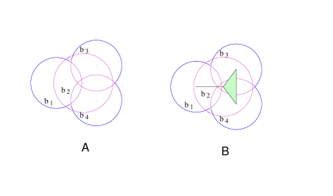
Figure 6.4: An example of analytical area calculation. (a) Area can be computed using the direct inclusion-exclusion. (b) The formula is simplified without any redundant terms when using alpha shape.

An example. An example of area computation by alpha shape is shown in Fig 6.4. Let $b_{1},b_{2},b_{3},b_{4}$ be the four disks. To simplify the notation we write $A_{i}$ for the area of $b_{i}$, $A_{ij}$ for the area of $b_{i}\cap b_{j}$, and $A_{ijk}$ for the area of $b_{i}\cap b_{j}\cap b_{k}$. The total area of the union, $b_{1}\cup b_{2}\cup b_{3}\cup b_{4}$, is

$$A_{\mbox{total}} = (A_{1}+A_{2}+A_{3}+A_{4})$$

$$- (A_{12}+A_{23}+A_{24}+A_{34})$$

$$+ A_{234}.$$

We add the area of $b_{i}$ if the corresponding vertex belongs to the alpha complex (Fig 6.4), we subtract the area of $b_{i}\cap b_{j}$ if the corresponding edge belongs to the alpha complex, and we add the area of $b_{i}\cap b_{j}\cap b_{k}$ if the corresponding triangle belongs to the alpha complex. Note without the guidance of the alpha complex, the inclusion-exclusion formula may be written as:

$$A_{\mbox{total}} = (A_{1}+A_{2}+A_{3}+A_{4})$$

$$- (A_{12}+A_{13}+A_{14}+A_{23}+A_{24}+A_{34})$$

$$+ (A_{123}+A_{124}+A_{134}+A_{234})$$

$$- A_{1234}.$$

This contains 6 canceling redundant terms: $A_{13}=A_{123}$, $A_{14}=A_{124}$, and $A_{134}=A_{1234}$. Computing these terms would be wasteful. Such redundancy does not occur when we use the alpha complex: the part of the Voronoi regions contained in the respective atom balls for the redundant terms do not intersect. Therefore, the corresponding edges and triangles do not enter the alpha complex. In two dimensions, we have terms of at most three disk intersections, corresponding to triangles in the alpha complex. Similarly, in three dimensions the most complicated terms are intersections of four spherical balls, and they correspond to tetrahedra in the alpha complex.

Voids and pockets. Voids and pockets represent the concave regions of a protein surface. Because shape-complementarity is the basis of many molecular recognition processes, binding and other activities frequently occur in pocket or void regions of protein structures. For example, the majority of enzyme reactions take place in surface pockets or interior voids.

The topological structure of the alpha shape also offers an effective method for computing voids and pockets in proteins. Consider the Delaunay tetrahedra that are not included in the alpha shape. If we repeatedly merge any two such tetrahedra on the condition that they share a 2-simplex triangle, we will end up with discrete sets of tetrahedra. Some of them will be completely isolated from the outside, and some of them are connected to the outside by triangle(s) on the boundary of the alpha shape. The former corresponds to voids (or cavities) in proteins, the latter corresponds to pockets and depressions in proteins.

A pocket differs from a depression in that it must have an opening that is at least narrower than one interior cross-section. Formally, the discrete flow [24] explains the distinction between a depression and a pocket. In a two dimensional Delaunay triangulation, the empty triangles that are not part of the alpha shape can be classified into obtuse triangles and acute triangles. The largest angle of an obtuse triangle is more than 90 degrees, and the largest angle of an acute triangle is less than 90 degrees. An empty obtuse triangle can be regarded as a “source” of empty space that “flows” to its neighbor, and an empty acute triangle a “sink” that collects flow from its obtuse empty neighboring triangle(s). In Figure 6.5a, obtuse triangles 1, 3, 4 and 5 flow to the acute triangle 2, which is a sink. Each of the discrete empty spaces on the surface of protein can be organized by the flow systems of the corresponding empty triangles: Those that flow together belong to the same discrete empty space. For a pocket, there is at least one sink among the empty triangles. For a depression, all triangles are obtuse, and the discrete flow goes from one obtuse triangle to another, from the innermost region to outside the convex hull. The discrete flow of a depression therefore goes to infinity. Figure 6.5b gives an example of a depression formed by a set of obtuse triangles.

Once voids and pockets are identified, we can apply the inclusion-exclusion principle based on the simplices to compute the exact size measurement (e.g., volume and area) of each void and pocket [25, 24].

Figure 6.5: Discrete flow of empty space illustrated for two dimensional disks. (a) Discrete flow of a pocket. Triangles 1, 3, 4 and 5 are obtuse. The free volume flows to the “sink” triangle 2, which is acute. (b) In a depression, the flow is from obtuse triangles to the outside.

The distinction between voids and pockets depends on the specific set of atomic radii and the solvent radius. When a larger solvent ball is used, the radii of all atoms will be inflated by a larger amount. This could lead to two different outcomes. A void or pocket may become completely filled and disappear. On the other hand, the inflated atoms may not fill the space of a pocket, but may close off the opening of the pocket. In this case, a pocket becomes a void. A widely used practice in the past was to adjust the solvent ball and repeatedly compute voids, in the hope that some pockets will become voids and hence be identified by methods designed for cavity/void computation. The pocket algorithm [24] and tools such as CastP [26, 27] often makes this unnecessary.

6.3 Computation and software

Computing Delaunay tetrahedrization and Voronoi diagram. It is easier to discuss the computation of tetrahedrization first. The incremental algorithm developed in [28] can be used to compute the weighted tetrahedrization for a set of atoms of different radii. For simplicity, we sketch the outline of the algorithm below for two dimensional unweighted Delaunay triangulation.

The intuitive idea of the algorithm can be traced back to the original observation of Delaunay. For the Delaunay triangulation of a point set, the circumcircle of an edge and a third point forming a Delaunay triangle must not contain a fourth point. Delaunay showed that if all edges in a particular triangulation satisfy this condition, the triangulation is a Delaunay triangulation. It is easy to come up with an arbitrary triangulation for a point set. A simple algorithm to covert this triangulation to the Delaunay triangulation is therefore to go through each of the triangles, and make corrections using “flips” discussed below if a specific triangle contains an edge violating the above condition. The basic ingredients for computing Delaunay tetrahedrization are generalizations of these observations. We discuss the concept of locally Delaunay edge and the edge-flip primitive operation below.

Locally Delaunay edge. We say an edge $ab$ is locally Delaunay if either it is on the boundary of the convex hull of the point set, or if it belongs to two triangles $abc$ and $abd$, and the circumcircle of $abc$ does not contain $d$ (e.g., edge $cd$ in Fig 6.6a).

Figure 6.6: An illustration of locally Delaunay edge and flips. (a) For the quadrilateral $abcd$, edge $ab$ is not locally Delaunay, as the circumcircle passing through edge $ab$ and a third point $c$ contains a fourth point $d$. Edge $cd$ is locally Delaunay, as $b$ is outside the circumcircle $adc$. An edge-flip or 2-to-2 flip replaces edge $ab$ by edge $cd$, and replace the original two triangles $abc$ and $adb$ with two new triangles $acd$ and $bcd$. (b) When a new vertex is inserted, we replace the old triangle containing this new vertex with three new triangles. This is called 1-to3 flips.

Edge-flip. If $ab$ is not locally Delaunay (edge $ab$ in Fig 6.6a), then the union of the two triangles $abc\cup abd$ is a convex quadrangle $acbd$, and edge $cd$ is locally Delaunay. We can replace edge $ab$ by edge $cd$. We call this an edge-flip or 2-to-2 flip, as two old triangles are replaced by two new triangles.

We recursively check each boundary edge of the quadrangle $abcd$ to see if it is also locally Delaunay after replacing $ab$ by $cd$. If not, we recursively edge-flip it.

Incremental algorithm for Delaunay triangulation. Assume we have a finite set of points (namely, atom centers) ${\cal S}=\{{\mbox{\boldmath$z$}}_{1},{\mbox{\boldmath$z$}}_{2},\cdots,{\mbox{\boldmath$z$}}_{i},\cdots,{\mbox{\boldmath$z$}}_{n}\}$. We start with a large auxiliary triangle that contains all these points. We insert the points one by one. At all times, we maintain a Delaunay triangulation ${\cal D}_{i}$ upto insertion of point ${\mbox{\boldmath$z$}}_{i}$.

After inserting point ${\mbox{\boldmath$z$}}_{i}$, we search for the triangle $\tau_{i-1}$ that contains this new point. We then add ${\mbox{\boldmath$z$}}_{i}$ to the triangulation and split the original triangle $\tau_{i-1}$ into three smaller triangles. This split is called 1-to-3 flip, as it replaces one old triangle with three new triangles. We then check if each of the three edges in $\tau_{i-1}$ still satisfies the locally Delaunay requirement. If not, we perform a recursive edge-flip. This algorithm is summarized in Algorithm 1.

Algorithm 1 Delaunay triangulation

  Obtain random ordering of points $\{{\mbox{\boldmath$z$}}_{1},\cdots,{\mbox{\boldmath$z$}}_{n}\}$;

  for $i=1$ to $n$ do

     find $\tau_{i-1}$ such ${\mbox{\boldmath$z$}}_{i}\in\tau_{i-1}$;

     add ${\mbox{\boldmath$z$}}_{i}$, and split $\tau_{i-1}$ into three triangles (1-to-3 flip);

     while any edge $ab$ not locally Delaunay do

        flip $ab$ to other diagonal $cd$ (2-to-2 edge flip);

     end while

  end for

In ${{\mathbb{R}}}^{3}$, the algorithm of tetrahedrization becomes more complex, but the same basic ideas apply. In this case, we need to locate a tetrahedron instead of a triangle that contains the newly inserted point. The concept of locally Delaunay is replaced by the concept of locally convex, and there are flips different than the 2-to-2 flip in ${{\mathbb{R}}}^{3}$ [28]. Although an incremental approach, i.e., sequentially adding points, is not necessary for Delaunay triangulation in ${{\mathbb{R}}}^{2}$, it is necessary in ${{\mathbb{R}}}^{3}$ to avoid non-flippable cases and to guarantee that the algorithm will terminate. This incremental algorithm has excellent expected performance [28].

The computation of Voronoi diagram is conceptually easy once the Delaunay triangulation is available. We can take advantage of the mathematical duality and compute all of the Voronoi vertices, edges, and planar faces from the Delaunay tetrahedra, triangles, and edges. Because one point ${\mbox{\boldmath$z$}}_{i}$ may be an vertex of many Delaunay tetrahedra, the Voronoi region of ${\mbox{\boldmath$z$}}_{i}$ therefore may contain many Voronoi vertices, edges, and planar faces. The efficient quad-edge data structure can be used for software implementation [29].

Volume and area computation. Let $V$ and $A$ denote the volume and area of the molecule, respectively, ${\cal K_{0}}$ for the alpha complex, $\sigma$ for a simplex in ${\cal K}$, $i$ for a vertex, $ij$ for an edge, $ijk$ for a triangle, and $ijkl$ for a tetrahedron. The algorithm for volume and area computation can be written as Algorithm 2.

Algorithm 2 Volume and area measurement

  $V:=A:=0.0$;

  for all $\sigma\in{\cal K}$ do

     if $\sigma$ is a vertex $i$ then

        $V:=V+\operatorname{vol}(b_{i})$; $A:=A+\operatorname{area}(b_{i})$;

     end if

     if $\sigma$ is an edge $ij$ then

        $V:=V-\operatorname{vol}(b_{i}\cap b_{j})$; $A:=A-\operatorname{area}(b_{i}\cap b_{j})$;

     end if

     if $\sigma$ is a triangle $ijk$ then

        $V:=V+\operatorname{vol}(b_{i}\cap b_{j}\cap b_{k})$; $A:=A+\operatorname{area}(b_{i}\cap b_{j}\cap b_{k})$;

     end if

     if $\sigma$ is a tetrahedron $ijkl$ then

        $V:=V-\operatorname{vol}(b_{i}\cap b_{j}\cap b_{k}\cap b_{l})$; $A:=A-\operatorname{area}(b_{i}\cap b_{j}\cap b_{k}\cap b_{l})$;

     end if

  end for

Additional details of volume and area computation can be found in [20, 21].

Software. The software package Delcx for computing weighted Delaunay tetrahedrization, Mkalf for computing the alpha shape, Volbl for computing volume and area of both molecules and interior voids and be found at www.alphashape.org. The CastP webserver for pocket computation can be found at cast.engr.uic.edu. There are other studies that compute or use Voronoi diagrams of protein structures [30, 31, 32, 32], although not all computes the weighted version which allows atoms to have different radii.

In this short description of algorithm, we have neglected many details important for geometric computation. For example, the problem of how to handle geometric degeneracy, namely, when three points are co-linear, or when four points are co-planar. Interested readers should consult the excellent monograph by Edelsbrunner for a detailed treatise of these and other important topics in computational geometry [33].

6.4 Applications: Packing analysis.

An important application of the Voronoi diagram and volume calculation is the measurement of protein packing. Tight packing is an important feature of protein structure [6, 10], and is thought to play important roles in protein stability and folding dynamics [34]. The packing density of a protein is measured by the ratio of its van der Waals volume and the volume of the space it occupies. One approach is to calculate the packing density of buried residues and atoms using Voronoi diagram [6, 10]. This approach was also used to derive radii parameters of atoms [15].

Figure 6.7: Voids and pockets for a set of 636 proteins representing most of the known protein folds, and the scaling behavior of the geometric properties of proteins. (a) The number of voids and pockets detected with a 1.4 Å probe is linearly correlated with the number of residues in a protein. Only proteins with less than 1,000 residues are shown. Solid triangles and empty circles represent the pockets and the voids, respectively. (b) The van der Waals ($vdw$) volume and van der Waals area of proteins scale linearly with each other. Similarly, molecular surface ($ms$) volume also scales linearly with molecular surface area using a probe radius of 1.4Å. (Data not shown. Figure adapted after [35])

Based on the computation of voids and pockets in proteins, a detailed study surveying major representatives of all known protein structural folds showed that there is a substantial amount of voids and pockets in proteins [35]. On average, every 15 residues introduces a void or a pocket (Fig 6.7a). For a perfectly solid three-dimensional sphere of radius $r$, the relationship between volume $V=4\pi r^{3}/3$ and surface area $A=4\pi r^{2}$ is: $V\propto A^{3/2}$. In contrast, Figure 6.7b shows that the van der Waals volume scales linearly with the van der Waals surface areas of proteins. The same linear relationship holds irrespective of whether we relate molecular surface volume and molecular surface area, or solvent accessible volume and solvent accessible surface area. This and other scaling behavior point out that protein interior is not packed as tight as solid [35]. Rather, packing defects in the form of voids and pockets are common in proteins.

If voids and pockets are prevalent in proteins, an interesting question is what is then the origin of the existence of these voids and pockets. This question was studied by examining the scaling behavior of packing density and coordination number of residues through the computation of voids, pockets, and edge simplices in the alpha shapes of random compact chain polymers [36]. For this purpose, a 32-state discrete state model was used to generate a large ensemble of compact self-avoiding walks. This is a difficult task, as it is very challenging to generate a large number of independent conformations of very compact chains that are self-avoiding. The results in [36] showed that it is easy for compact random chain polymers to have similar scaling behavior of packing density and coordination number with chain length. This suggests that proteins are not optimized by evolution to eliminate voids and pockets, and the existence of many pockets and voids is random in nature, and is due to the generic requirement of compact chain polymers. The frequent occurrence and the origin of voids and pockets in protein structures raise a challenging question: How can we distinguish voids and pockets that perform biological functions such as binding from those formed by random chance? This question is related to the general problem of protein function prediction.

6.5 Applications: Protein function prediction from structures.

Conservation of protein structures often reveals very distant evolutionary relationship, which are otherwise difficult to detect by sequence analysis [37]. Comparing protein structures can provide insightful ideas about the biochemical functions of proteins (e.g., active sites, catalytic residues, and substrate interactions) [38, 39, 40].

A fundamental challenge in inferring protein function from structure is that the functional surface of a protein often involves only a small number of key residues. These interacting residues are dispersed in diverse regions of the primary sequences and are difficult to detect if the only information available is the primary sequence. Discovery of local spatial motifs from structures that are functionally relevant has been the focus of many studies.

Graph based methods for spatial patterns in proteins. To analyze local spatial patterns in proteins. Artymiuk et al developed an algorithm based on subgraph isomorphism detection [41]. By representing residue side-chains as simplified pseudo-atoms, a molecular graph is constructed to represent the patterns of side-chain pseudo-atoms and their inter-atomic distances. A user defined query pattern can then be searched rapidly against the Protein Data Bank for similarity relationship. Another widely used approach is the method of geometric hashing. By examining spatial patterns of atoms, Fischer et al developed an algorithm that can detect surface similarity of proteins [42, 43]. This method has also been applied by Wallace et al for the derivation and matching of spatial templates [44]. Russell developed a different algorithm that detects side-chain geometric patterns common to two protein structures [45]. With the evaluation of statistical significance of measured root mean square distance, several new examples of convergent evolution were discovered, where common patterns of side-chains were found to reside on different tertiary folds.

These methods have a number of limitations. Most require a user-defined template motif, restricting their utility for automated database-wide search. In addition, the size of the spatial pattern related to protein function is also often restricted.

Predicting protein functions by matching pocket surfaces. Protein functional surfaces are frequently associated with surface regions of prominent concavity [46, 26]. These include pockets and voids, which can be accurately computed as we have discussed. Computationally, one wishes to automatically identify voids and pockets on protein structures where interactions exist with other molecules such as substrate, ions, ligands, or other proteins.

Binkowski et al. developed a method for predicting protein function by matching a surface pocket or void on a protein of unknown or undetermined function to the pocket or void of a protein of known function [47, 48]. Initially, the Delaunay tetrahedrization and alpha shapes for almost all of the structures in the PDB databank are computed [27]. All surface pockets and interior voids for each of the protein structure are then exhaustively computed [24, 25]. For each pocket and void, the residues forming the wall are then concatenated to form a short sequence fragment of amino acid residues, while ignoring all intervening residues that do not participate in the formation of the wall of the pocket or void. Two sequence fragments, one from the query protein and another from one of the proteins in the database, both derived from pocket or void surface residues, are then compared using dynamic programming. The similarity score for any observed match is assessed for statistical significance using an empirical randomization model constructed for short sequence patterns.

For promising matches of pocket/void surfaces showing significant sequence similarity, we can further evaluate their similarity in shape and in relative orientation. The former can be obtained by measuring the coordinate root mean square distance (rmsd) between the two surfaces. The latter is measured by first placing a unit sphere at the geometric center ${\mbox{\boldmath$z$}}_{0}\in{{\mathbb{R}}}^{3}$ of a pocket/void. The location of each residue ${\mbox{\boldmath$z$}}=(x,y,z)^{T}$ is then projected onto the unit sphere along the direction of the vector from the geometric center: ${\mbox{\boldmath$u$}}=({\mbox{\boldmath$z$}}-{\mbox{\boldmath$z$}}_{0})/||{\mbox{\boldmath$z$}}-{\mbox{\boldmath$z$}}_{0}||$. The projected pocket is represented by a collection of unit vectors located on the unit sphere, and the original orientation of residues in the pocket is preserved. The rmsd distance of the two sets of unit vectors derived from the two pockets are then measured, which is called the ormsd for orientation rmsd [47]. This allows similar pockets with only minor conformational changes to be detected [47].

The advantage of the method of Binkowski et al is that it does not assume prior knowledge of functional site residues, and does not require a priori any similarity in either the full primary sequence or the backbone fold structures. It has no limitation in the size of the spatially derived motif and can successfully detect patterns small and large. This method has been successfully applied to detect similar functional surfaces among proteins of the same fold but low sequence identities, and among proteins of different fold [47, 49].

Function prediction through models of protein surface evolution. To match local surfaces such as pockets and voids and to assess their sequence similarity, an effective scoring matrix is critically important. In the original study of Binkowski et al, Blosum matrix was used. However, this is problematic, as Blosum matrices were derived from analysis of precomputed large quantities of sequences, while the information of the particular protein of interest has limited or no influence. In addition, these precomputed sequences include buried residues in protein core, whose conservation reflects the need to maintain protein stability rather than to maintain protein function. In reference [50, 51], a continuous time Markov process was developed to explicitly model the substitution rates of residues in binding pockets. Using a Bayesian Markov chain Monte Carlo method, the residue substitution rates at functional pocket are estimated. The substitution rates are found to be very different for residues in the binding site and residues on the remaining surface of proteins. In addition, substitution rates are also very different for residues in the buried core and residues on the solvent exposed surfaces.

These rates are then used to generate a set of scoring matrices of different time intervals for residues located in the functional pocket. Application of protein-specific and region-specific scoring matrices in matching protein surfaces result in significantly improved sensitivity and specificity in protein function prediction [50, 51].

In a large scale study of predicting protein functions from structures, a subset of 100 enzyme families are collected from the total of 286 enzyme families containing between 10–50 member protein structures with known Enzyme Classification (E.C.) labels. By estimating the substitution rate matrix for residues on the active site pocket of a query protein, a series of scoring matrices of different evolutionary time is derived. By searching for similar pocket surfaces from a database of 770,466 pockets derived from the CastP database (with the criterion that each must contain at least 8 residues), this method can recover active site surfaces on enzymes similar to that on the query structure at an accuracy of $>92$%. Fig 6.8 shows the Receiver Operating Characteristic Curve of this study. An example of identifying human amylase using template surfaces from B. subtilis and from barley is shown in Fig 6.9.

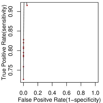
Figure 6.8: A large scale study of protein function prediction from structures by matching similar functional surfaces for 100 protein families. A correct prediction is made if the matched surface comes from a protein structure with the same Enzyme Classification (E.C.) number (upto the 4-th digit) as that of the query protein. The $x$-axis of the Receiver Operating Characteristics curve reflects the false positive rate ($1-$specificity) at different statistical significance $p$-value by cRMSD measurement, and the $y$-axis reflects the true positive rate (sensitivity).

The method of surface matching based on evolutionary model is also especially effective in solving the challenging problems of protein function prediction of orphan structures of unknown function (such as those obtained in structural genomics projects), which have only sequence homologs that are themselves hypothetical proteins with unknown functions.

Figure 6.9: Protein function prediction as illustrated by the example of alpha amylases. Two template binding surfaces are used to search database of protein surfaces to identify protein structures that are of similar functions. (a) The phylogenetic tree for the template Pdb structure 1bag from B. subtilis. (b) The template binding pocket of alpha amylase on 1bag. (c) A matched binding surface on a different protein structure (1b2y from human, full sequence identity 22%) obtained by querying with 1bag. (d) The phylogenetic tree for the template structure 1bg9 from H. vulgare. (e) The template binding pocket on 1bg9. (f) A matched binding surface on a different protein structure (1u2y from human, full sequence identity 23%) obtained by querying with 1bg9 (Adapted from [51]).

6.6 Discussion

A major challenge in studying protein geometry is to understand our intuitive notions of various geometric aspects of molecular shapes, and to quantify these notions with mathematical models that are amenable to fast computation. The advent of the union of ball model of protein structures enabled rigorous definition of important geometric concepts such as solvent accessible surface and molecular surface. It also led to the development of algorithms for area and volume calculations of proteins. Deep understanding of the topological structure of molecular shapes is also based on the idealized union of ball model [9]. A success in approaching these problems is exemplified in the development of the pocket algorithm [24]. Another example is the recent development of a rigorous definition of protein-protein binding or interaction interface and algorithm for its computation [52].

Perhaps a more fundamental problem we face is to identify important structural and chemical features that are the determinants of biological problems of interest. For example, we would like to know what are the shape features that has significant influences on protein solvation, protein stability, ligand specific binding, and protein conformational changes. It is not clear whether our current geometric intuitions are sufficient, or are the correct or the most relevant ones. There may still be important unknown shape properties of molecules that elude us at the moment.

An important application of geometric computation of protein structures is to detect patterns important for protein function. The shape of local surface regions on a protein structure and their chemical texture are the basis of its binding interactions with other molecules. Proteins fold into specific native structure to form these local regions for carrying out various biochemical functions. The geometric shape and chemical pattern of the local surface regions, and how they change dynamically are therefore of fundamental importance in computational studies of proteins.

Another important application is the development of geometric potential functions. Potential functions are important for generating conformations, for distinguishing native and near native conformations from other decoy conformations in protein structure predictions [53, 54, 55, 56] and in protein-protein docking [57]. They are also important for peptide and protein design [57, 58]. Chapter 4 describes in details the development of geometric potential and applications in decoy discrimination and in protein-protein docking prediction.

We have not described in detail the approach of studying protein geometry using graph theory. In addition to side-chain pattern analysis briefly discussed earlier, graph based protein geometric model also has lead to a number of important insights, including the optimal design of model proteins formed by hydrophobic and polar residues [59], and methods for optimal design of side-chain packing [60, 61]. Another important topic we did not touch upon is the analysis of the topology of protein backbones. Based on concepts from knot theory, Røgen and Bohr developed a family of global geometric measures for protein structure classification [62]. These measures originate from integral formulas of Vassiliev knot invariants. With these measures, Røgen and Fain further constructed a system that can automatically classify protein chains into folds [63]. This system can reproduce the Cath classification system that requires explicit structural alignment as well as human curation.

Further development of descriptions of geometric shape and topological structure, as well as algorithms for their computation will provide a solid foundation for studying many important biological problems. The other important tasks are then to show how these descriptors may be effectively used to deepen our biological insights and to develop accurate predictive models of biological phenomena. For example, in computing protein-protein interfaces, a challenging task is to discriminate surfaces that are involved in protein binding from other non-binding surface regions, and to understand in what fashion this depends on the properties of the binding partner protein.

Undoubtedly, evolution plays central roles in shaping up the function and stability of protein molecules. The method of analyzing residue substitution rates using a continuous time Markov models [50, 51], and the method of surface mapping of conservation entropy and phylogeny [64, 65] only scratches the surface of this important issue. Much remains to be done in incorporating evolutionary information in protein shape analysis for understanding biological functions.

6.7 Summary

The accumulation of experimentally solved molecular structures of proteins provides a wealth of information for studying many important biological problems. With the development of a rigorous model of the structure of protein molecules, various shape properties, including surfaces, voids, and pockets, and measurements of their metric properties can be computed. Geometric algorithms have found important applications in protein packing analysis, in developing potential functions, in docking, and in protein function prediction. It is likely further development of geometric models and algorithms will find important applications in answering additional biological questions.

6.8 Further reading

The original work of Lee and Richards surface can be found in [5], where they also formulated the molecular surface model [8]. Michael Connolly developed the first method for the computation of the molecular surface [11]. Tsai et al. described a method for obtaining atomic radii parameter [15]. The mathematical theory of the union of balls and alpha shape was developed by Herbert Edelsbrunner and colleague [9, 66]. Algorithm for computing weighted Delaunay tetrahedrization can be found in [28], or in a concise monograph with in-depth discussion of geometric computing [33]. Details of area and volume calculations can be found in [20, 21, 25]. The theory of pocket computation and applications can be found in [24, 26]. Richards and Lim offered a comprehensive review on protein packing and protein folding [12]. A detailed packing analysis of proteins can be found in [35]. The study on inferring protein function by matching surfaces is described in [47]. The study of the evolutionary model of protein binding pocket and its application in protein function prediction can be found in [51].

6.9 Acknowledgments

This work is supported by grants from the National Science Foundation (CAREER DBI0133856), the National Institute of Health (GM68958), the Office of Naval Research (N000140310329), and the Whitaker Foundation (TF-04-0023). The author thanks Jeffrey Tseng for help in preparing this chapter.

Bibliography

- [1] G. Rhodes. Crystallography Made Crystal Clear: A Guide for Users of Macromolecular Models. Academic Press, 1999.
- [2] G. M. Crippen and T. F. Havel. Distance Geometry and Molecular Conformation. J. Wiley & Sons, 1988.
- [3] W. Rieping, M. Habeck, and M. Nilges. Inferential structure determination. Science, 309(5732):303–6, 2005.
- [4] R.F.W. Bader. Atoms in Molecules: A Quantum Theory. The international series of mongraphs on chemistry, No. 22. Oxford University Press, 1994.
- [5] B. Lee and F. M. Richards. The interpretation of protein structures: estimation of static accessibility. J. Mol. Biol., 55:379–400, 1971.
- [6] F. M. Richards. The interpretation of protein structures: total volume, group volume distributions and packing density. J. Mol. Biol., 82:1–14, 1974.
- [7] T. J. Richmond. Solvent accessible surface area and excluded volume in proteins: analytical equations for overlapping spheres and implications for the hydrophobic effect. J. Mol. Biol., 178:63–89, 1984.
- [8] F. M. Richards. Calculation of molecular volumes and areas for structures of known geometries. Methods in Enzymology, 115:440–464, 1985.
- [9] H. Edelsbrunner. The union of balls and its dual shape. Discrete Comput. Geom., 13:415–440, 1995.
- [10] F. M. Richards. Areas, volumes, packing, and protein structures. Ann. Rev. Biophys. Bioeng., 6:151–176, 1977.
- [11] M. L. Connolly. Analytical molecular surface calculation. J. Appl. Cryst., 16:548–558, 1983.
- [12] F. M. Richards and W. A. Lim. An analysis of packing in the protein folding problem. Q. Rev. Biophys., 26:423–498, 1994.
- [13] M. Gerstein and F. M Richards. Protein Geometry: Distances, Areas, and Volumes, volume F, chapter 22. International Union of Crystallography, 1999.
- [14] F. M. Richards. The interpretation of protein structures: total volume, group volume distributions and packing density. J. Mol. Biol., 82:1–14, 1974.
- [15] J. Tsai, R. Taylor, C. Chothia, and M. Gerstein. The packing density in proteins: standard radii and volumes. J Mol Biol, 290(1):253–66, 1999.
- [16] A. Bondi. VDW volumes and radii. J. Phys. Chem., 68:441–451, 1964.
- [17] J.M. Word, S.C. Lovell, J.S. Richardson, and D.C. Richardson. Asparagine and glutamine: using hydrogen atom contacts in the choice of side-chain amide orientation. J Mol Biol, 285(4):1735–47, 1999.
- [18] J. L. Finney. Volume occupation, environment and accessibility in proteins. The problem of the protein surface. J. Mol. Biol., 96:721–732, 1975.
- [19] B. J. Gellatly and J.L. Finney. Calculation of protein volumes: an alternative to the Voronoi procedure. J. Mol. Biol., 161:305–322, 1982.
- [20] H. Edelsbrunner, M. Facello, P. Fu, and J. Liang. Measuring proteins and voids in proteins. In Proc. 28th Ann. Hawaii Int’l Conf. System Sciences, volume 5, pages 256–264, Los Alamitos, California, 1995. IEEE Computer Scociety Press.
- [21] J. Liang, H. Edelsbrunner, P. Fu, P. V. Sudhakar, and S. Subramaniam. Analytical shape computing of macromolecules I: Molecular area and volume through alpha-shape. Proteins, 33:1–17, 1998.
- [22] K. W. Kratky. Intersecting disks (and spheres) and statistical mechanics. I. mathematical basis. J. Stat. Phys., 25:619–634, 1981.
- [23] M. Petitjean. On the analytical calculation of van der waals surfaces and volumes: some numerical aspects. J. Comput. Chem., 15:507–523, 1994.
- [24] H. Edeslbrunner, M. Facello, and J. Liang. On the definition and the construction of pockets in macromolecules. Disc. Appl. Math., 88:18–29, 1998.
- [25] J. Liang, H. Edelsbrunner, P. Fu, P. V. Sudhakar, and S. Subramaniam. Analytical shape computing of macromolecules II: Identification and computation of inaccessible cavities inside proteins. Proteins, 33:18–29, 1998.
- [26] J. Liang, H. Edelsbrunner, and C. Woodward. Anatomy of protein pockets and cavities: Measurement of binding site geometry and implications for ligand design. Protein Sci, 7:1884–1897, 1998.
- [27] T. A. Binkowski, S. Naghibzadeh, and J. Liang. CASTp: Computed atlas of surface topography of proteins. Nucleic Acids Res., 31:3352–3355, 2003.
- [28] H. Edelsbrunner and N.R. Shah. Incremental topological flipping works for regular triangulations. Algorithmica, 15:223–241, 1996.
- [29] L. Guibas and J. Stolfi. Primitives for the manipulation of general subdivisions and the computation of Voronoi diagrams. ACM Transactions on Graphiques, 4:74–123, 1985.
- [30] S. Chakravarty, A. Bhinge, and R. Varadarajan. A procedure for detection and quantitation of cavity volumes proteins. application to measure the strength of the hydrophobic driving force in protein folding. J Biol Chem, 277(35):31345–53, 2002.
- [31] A. Goede, R. Preissner, and C. Frommel. Voronoi cell: New method for allocation of space among atoms: Elimination of avoidable errors in calculation of atomic volume and density. J. Comput. Chem., 18:1113–1123, 1997.
- [32] Y. Harpaz, M. Gerstein, and C. Chothia. Volume changes on protein folding. Structure, 2(7):641–9, 1994.
- [33] H. Edelsbrunner. Geometry and Topology for Mesh Generation. Cambridge University Press, 2001.
- [34] M. Levitt, M. Gerstein, E. Huang, S. Subbiah, and J. Tsai. Protein folding: the endgame. Annu Rev Biochem, 66:549–579, 1997.
- [35] J. Liang and K. A. Dill. Are proteins well-packed? Biophys. J., 81:751–766, 2001.
- [36] J. Zhang, R. Chen, C. Tang, and J. Liang. Origin of scaling behavior of protein packing density: A sequential monte carlo study of compact long chain polymers. J. Chem. Phys., 118:6102–6109, 2003.
- [37] A. E. Todd, C. A. Orengo, and J. M. Thornton. Evolution of function in protein superfamilies, from a structural perspective. J. Mol. Biol., 307:1113–1143, 2001.
- [38] L. Holm and C. Sander. New structure: Novel fold? Structure, 5:165–171, 1997.
- [39] A. C. R. Martin, C. A. Orengo, E. G. Hutchinson, A. D. Michie, A. C. Wallace, M. L. Jones, and J. M. Thornton. Protein folds and functions. Structure, 6:875–884, 1998.
- [40] C. A. Orengo, A. E. Todd, and J. M. Thornton. From protein structure to function. Curr. Opinion Structural Biology, 9(4):374–382, 1999.
- [41] P. J. Artymiuk, A. R. Poirrette, H. M. Grindley, D.W. Rice, and P. Willett. A graph-theoretic approach to the identification of three-dimensional patterns of amino acid side-chains in protein structure. J. Mol. Biol., 243:327–344, 1994.
- [42] D. Fischer, R. Norel, H. Wolfson, and R. Nussinov. Surface motifs by a computer vision technique: searches, detection, and implications for protein- ligand recognition. Proteins: Structure, Function and Genetics, 16:278–292, 1993.
- [43] R. Norel, D. Fischer, H. J. Wolfson, and R. Nussinov. Molecualr surface recognition by computer vision-based technique. Protein Eng., 1994.
- [44] A. C. Wallace, N. Borkakoti, and J. M. Thornton. TESS: a geometric hashing algorithm for deriving 3d coordinate templates for searching structural databases. Application to enzyme active sites. Protein Sci., 6:2308–2323, 1997.
- [45] R. Russell. Detection of protein three-dimensional side-chain patterns: New examples of convergent evolution. J. Mol. Biol., 279:1211–1227, 1998.
- [46] R. A. Laskowski, N. M. Luscombe, M. B. Swindells, and J. M. Thornton. Protein clefts in molecular recognition and function. Protein Sci., 5:2438–2452, 1996.
- [47] T. A. Binkowski, L. Adamian, and J. Liang. Inferring functional relationship of proteins from local sequence and spatial surface patterns. J. Mol. Biol., 332:505–526, 2003.
- [48] T.A. Binkowski, A. Joachimiak, and J. Liang. Protein surface analysis for function annotation in high-throughput structural genomics pipeline. Protein Sci, 14(12):2972–81, 2005.
- [49] T.A. Binkowski, P. Freeman, and J. Liang. pvSOAR: Detecting similar surface patterns of pocket and void surfaces of amino acid residues on proteins. Nucleic Acid Research, 32:W555–W558, 2004.
- [50] Y.Y. Tseng and J. Liang. Estimating evolutionary rate of local protein binding surfaces: a bayesian monte carlo approach. Proceedings of 2005 IEEE-EMBC Conference, 2005.
- [51] Y.Y. Tseng and J. Liang. Estimation of amino acid residue substitution rates at local spatial regions and application in protein function inference: A Bayesian Monte Carlo approach. Mol. Biol. Evol., 23:421–436, 2006.
- [52] Y. Ban, H. Edelsbrunner, and J. Rudolph. Interface surfaces for protein-protein complexes. In RECOMB, pages 205–212, 2004.
- [53] R. K. Singh, A. Tropsha, and I. I. Vaisman. Delaunay tessellation of proteins: four body nearest-neighbor propensities of amino-acid residues. J. Comp. Bio., 3:213–221, 1996.
- [54] W. Zheng, S. J. Cho, I. I. Vaisman, and A. Tropsha. A new approach to protein fold recognition based on Delaunay tessellation of protein structure. In R.B. Altman, A.K. Dunker, L. Hunter, and T.E. Klein, editors, Pacific Symposium on Biocomputing’97, pages 486–497, Singapore, 1997. World Scientific.
- [55] X. Li, C. Hu, and J. Liang. Simplicial edge representation of protein structures and alpha contact potential with confidence measure. Proteins, 53:792–805, 2003.
- [56] X. Li and J. Liang. Geometric cooperativity and anticooperativity of three-body interactions in native proteins. Proteins, 60(1):46–65, 2005.
- [57] X. Li and J. Liang. Computational design of combinatorial peptide library for modulating protein-protein interactions. Pac Symp Biocomput, pages 28–39, 2005.
- [58] C. Hu, X. Li, and J. Liang. Developing optimal nonlinear scoring function for protein design. Bioinformatics, 20:3080–3098, 2004.
- [59] J. Kleinberg. Efficient algorithms for protein sequence design and the analysis of certain evolutionary fitness landscapes. In RECOMB, pages 205–212, 2004.
- [60] J. Xu. Rapid protein side-chain packing via tree decomposition. In RECOMB, pages 423–439, 2005.
- [61] A. Leaver-Fay, B. Kuhlman, and J. Snoeyink. An adaptive dynamic programming algorithm for the side chain placement problem. In Pacific Symposium on Biocomputing, pages 17–28, 2005.
- [62] P. Røgen and H. Bohr. A new family of global protein shape descriptors. Math Biosci, 182(2):167–81, 2003.
- [63] P. Røgen and B. Fain. Automatic classification of protein structure by using gauss in tegrals. Proc Natl Acad Sci U S A, 100(1):119–24, 2003.
- [64] O. Lichtarge, H.R. Bourne, and F.E. Cohen. An evolutionary trace method defines binding surfaces common to protein families. J Mol Biol, 257(2):342–58, 1996.
- [65] F. Glaser, T. Pupko, I. Paz, R.E. Bell, D. Shental, E. Martz, and N. Ben-Tal. Consurf: identification of functional regions in proteins by surface-mapping of phylogenetic information. Bioinformatics, 19(1):163–4, 2003.
- [66] H. Edelsbrunner and E.P. Mücke. Three-dimensional alpha shapes. ACM Trans. Graphics, 13:43–72, 1994.