The Topology of Pseudoknotted Homopolymers

Abstract

We consider the folding of a self-avoiding homopolymer on a lattice, with saturating hydrogen bond interactions. Our goal is to numerically evaluate the statistical distribution of the topological genus of pseudoknotted configurations. The genus has been recently proposed for classifying pseudoknots (and their topological complexity) in the context of RNA folding. We compare our results on the distribution of the genus of pseudoknots, with the theoretical predictions of an existing combinatorial model for an infinitely flexible and stretchable homopolymer. We thus obtain that steric and geometric constraints considerably limit the topological complexity of pseudoknotted configurations, as it occurs for instance in real RNA molecules. We also analyze the scaling properties at large homopolymer length, and the genus distributions above and below the critical temperature between the swollen phase and the compact-globule phase, both in two and three dimensions.

One of the most exciting fields in modern computational molecular biology is the search for tools predicting the complex foldings of bio-polymers such as RNA SBS ; tinoco ; Higgs , when homologous sequences are not available.

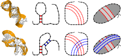
Figure 1: Top, from left to right: a hairpin loop (PDB number 1NA2), its squiggle-plot and disk diagram representation which is of genus zero since it is planar. Bottom: $H$-type pseudoknot (PDB number 1RNK). In this case the disk diagram is not planar and has genus one.

The prediction of the full tertiary structure of a RNA molecule is still an open issue mfold , mainly because of its intrinsic high computational complexity lyngso . It is known that the tertiary structure involves an important set of structural motifs, the so-called pseudoknots Bosch . These are conformations such that the associated disk diagram (which represents all nucleotides along the RNA backbone as points on an oriented circle from the 5’ end to the 3’ end, and where each base-pair is represented by an arc joining the two interacting nucleotides, inside the circle; see Figure 1) is not planar, i.e. it contains intersecting arcs. RNA pseudoknots have been identified in nearly every organism, and they proved to play important regulatory and functional roles c1 ; c2 . Their ubiquity manifests in a large variety of possible shapes and structures plos , and their existence should not be neglected in structure prediction algorithms, as they account for the 10%-30% on average of the total number of base pairs. Actually, several computer programs have been proposed for predicting RNA secondary structures including pseudoknots eddyrivas ; POZ ; PTOZ ; HI ; Gul ; abrah ; Tab (the list is not exhaustive), but the complexity of the problem and the approximations involved are usually such that the issue is far from being solved eddyBIO .
An analytic mathematical tool which can fully describe any RNA contact structure including all possible pseudoknots, appeared first in OZ . There, all RNA disk diagrams are considered as Feynman diagrams of a suitable field theory of $N\times N$ Hermitian matrices (a combinatorial tool borrowed from quantum field theory). The latter is known to organize all the diagrams according to an asymptotic $1/N^{2}$ topological expansion at large-$N$ thooft . This provides in fact a rigorous way to classify non-planar diagrams, and therefore it induces a natural topological classification of pseudoknots PTOZ . Namely, to any given pseudoknotted configuration (and more generally, to any contact structure of an heteropolymer with binary saturating interactions), one can associate an integer number $g$, the genus. It is defined as the topological genus of the associated disk diagram, i.e. by $\chi=1-2g$ where $\chi$ is the Euler characteristic number of the diagram. As reviewed in VOZ , the genus is the minimum number of handles the disk should have in order that all the cords are not intersecting (see Figure 1). Other characterizations of pseudoknots have been proposed (e.g. stella ; Aeddy ; Lucas ). The classification OZ is truly topological, meaning that it is independent from the way the diagram is drawn, and dependent only on the intrinsic complexity of the contact structure.

The large-$N$ asymptotics of the analytical model in OZ is hard to obtain exactly. However, in PRL a special case of the general model OZ has been considered and solved. It was the simple case of an infinitely flexible and stretchable homopolymer, where there is no dependence on the primary sequence, and any saturating base pair between all the “nucleotides” is allowed. An analytical asymptotic expansion was evaluated and the distribution of the genus of pseudoknotted contact structures was obtained. One of the results is that an homopolymer with $L$ nucleotides has an average genus close to the maximal one, that is $L/4$. Of course, real RNA molecules are not infinitely flexible and stretchable homopolymers. It is customary to assume that the bases $i$ and $j$ can interact only if they are sufficiently far apart along the chain (e.g. $\left|i-j\right|\geq 4$, mfold ) because of bending rigidity. Moreover helices have a long persistence length ($\sim 200$ base pairs) and this necessarily constrains the allowed pairings even more. We expect that including all steric and geometrical constraints should considerably decrease the genus of allowed pseudoknots, compared to the purely combinatorial case PRL where the actual three-dimensional conformation was neglected. The purpose of this Letter is to numerically analyze the effects of steric and geometric constraints on the genus distribution of pseudoknots topologies in homopolymers, in the same spirit of PRL .

The Model: we model the system by considering a polymer on a cubic lattice, i.e. a self-avoiding random walk with short-range attractive interaction degennes . A self-avoiding walk (SAW) is a sequence of neighboring lattice sites $i=0,1,\ldots,n$ with coordinates $\{\mathbf{r}_{i}\}$, such that the same lattice-site cannot be visited more than once. This is a standard approach in polymer physics (and RNA: see e.g. stella ; Lucas ). The attractive interaction is usually used to describe bad solvent quality, but in our case we insist more on the saturating nature of the hydrogen bond interactions. Such a requirement is crucial here, since the concept of the topological genus for a contact structure can be defined unambiguously only when the interactions are saturating. One of the most natural ways to model the interaction is by considering a “spin” model (see e.g. GOO ; FS ; Tiana ). Strictly speaking, our model is a variation of the standard $\theta$-polymer model, and similar interaction models for RNA on the lattice have been already proposed (e.g. orl ). To each vertex $i$ we associate a unit spin $\mathbf{s}_{i}$ which represents the nucleotide direction with respect to the backbone. The only allowed directions for $\mathbf{s}_{i}$ are the lattice ones. Moreover, the spins cannot overlap with the backbone because of the excluded volume between the nucleotides and the backbone. The saturating nucleotide-nucleotide interaction occurs when two spins $\mathbf{s}_{i},\mathbf{s}_{j}$ on neighboring sites, $\left|\mathbf{r}_{i}-\mathbf{r}_{j}\right|=1$, are pointing to each other. The energy of a configuration $\{\mathbf{r}_{i},\mathbf{s}_{i}\}$ is thus defined by the Hamiltonian:

$${\mathcal{H}}=-\epsilon\sum_{i<j}\,\delta(\mathbf{r}_{i}+\mathbf{s}_{i}-\mathbf{r}_{j})\delta(\mathbf{s}_{i}+\mathbf{s}_{j})\delta(\left|\mathbf{r}_{i}-\mathbf{r}_{j}\right|-1)\,,$$ (1)

where $\epsilon\geq 0$ is an effective hydrogen-binding energy, the same for all monomers of the chain. Let us note that since we are not aimidgng to set up a realistic lattice model for RNA-folding, but rather to understand steric effects on the genus distributions of a homopolymer, we do not take into account stacking energies.

The basic features of our model are clear: At high temperatures, we expect the system to be in a swollen SAW state (entropy dominated coil state), whereas at lower temperatures we expect a kind of “compact globule”-like phase degennes . The transition temperature $T_{\theta}$ defines the so-called $\theta$-point. However, details on the thermodynamics, kinetics, phase diagram, etc. can be rather complex orl ; Lucas . We limit ourselves here only to the analysis of the genus distribution of pseudoknotted structures for comparing the effects of stericity constraints versus the purely combinatorial model of PRL . All other considerations are postponed elsewhere.

The Method: The numerical sampling of the statistical distribution ${\mathcal{Z}}=\sum_{\mathrm{SAW},\{\mathbf{s}_{i}\}}\exp({-\mathcal{H}/k_{B}T})$, where $k_{B}$ is Boltzmann’s constant, $T$ is the absolute temperature, and the sum is restricted to SAWs and configurations of spins $\{\mathbf{s}_{i}\}$ satisfying the aforementioned constraints, is implemented by using the Monte Carlo Growth Method. It was originally proposed by T. Garel and H. Orland in GO and has been applied to several statistical systems since then (see references in HO ). It consists in starting with an ensemble of chains at equilibrium and then growing each chain by adding one monomer at a time with a probability proportional to the Boltzmann factor for the energy of the chain. At each step the ensemble remains at equilibrium (a detailed description of the algorithm with applications can be found in HO ). It belongs to the family of so-called “population Monte Carlo algorithms” Iba , where, contrary to the “dynamical” Markov Chain Monte Carlo methods, the population is fully grown and evolved, non-dynamically. At high temperatures we considered populations with a variable number of chains in the range 10000-40000, and with a typical length of $L=500$ monomers (up to $L=1200$ in some cases). Accuracy and statistical averages were computed by taking several independent populations (of the order of 40). At low temperatures we considered populations of up to 100000 chains. All the simulations have also been performed on a square lattice in two dimensions.

Results and discussion: We expect different genus distributions above and below $T_{\theta}$. We therefore first determine $T_{\theta}$ , which can be done efficiently by computing the end-to-end distance $R_{e}^{2}=(\mathbf{r}_{L}-\mathbf{r}_{0})^{2}$, and the radius of gyration $R_{g}^{2}=\sum_{i<j}(\mathbf{r}_{i}-\mathbf{r}_{j})^{2}/L^{2}$. It is known that the ratio $\rho^{2}=\langle R_{e}^{2}\rangle/\langle R_{g}^{2}\rangle$ is universal in the limit $L\to\infty$ and converges to a step function as a function of $T$, with a universal critical value at $T_{\theta}$ degennes ; PHA ; Nickel . In Figure 2 we plot $\rho$ which shows a transition temperature $T_{\theta}=0.39\pm 0.01$ ($T^{2D}_{\theta}=0.48\pm 0.02$ in two dimensions), in units where $k_{B}=1$ and $\epsilon=1$.

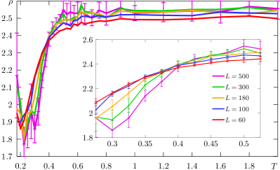
Figure 2: The ratio $\rho$ in $3d$ as a function of the temperature $T$, for several values of $L$ (with error bars plotted only for $L=60$). At low temperatures the error bars are larger than the variations of the curves. The inset shows that as $L$ increases, the curves approach a universal step function about $T_{\theta}\sim 0.39\pm 0.01$.

We also verified that $\rho_{\infty}=2.5\pm 0.05$ for $T\gg T_{\theta}$ asymptotically, and we find an intermediate value $\rho_{\theta}=2.35\pm 0.05$ at $T_{\theta}$ (and $\rho_{\infty}=2.67\pm 0.01$ and $\rho_{\theta}=2.39\pm 0.01$ in 2d, respectively). At large-$L$ we find the following scalings: for $T>T_{\theta}$, $\langle R_{g}\rangle\sim L^{\nu}$ with $\nu=0.59\pm 0.01$ ($\nu=0.75\pm 0.02$ in two dimensions), which is consistent with the critical exponent of a swollen SAW; for $T<T_{\theta}$, $\nu=0.32\pm 0.02$ ($\nu=0.50\pm 0.01$ in two dimensions) which is consistent with a compact phase. All these results are in agreement with high-accuracy simulations of similar models grassberger ; madras . We then proceed with extracting the genus distributions in the two phases. The results are in Figure 3 and 4.

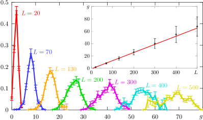
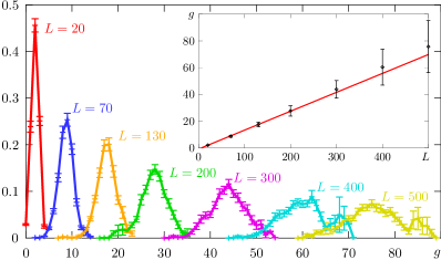
Figure 3: The genus distributions of pseudoknots at fixed $L$, in $2d$ (top) and $3d$ (bottom), in the compact phase at $T=0.225$ and $T=0.2$, respectively. The insets represent the behavior of $\langle g\rangle$ at large-$L$.

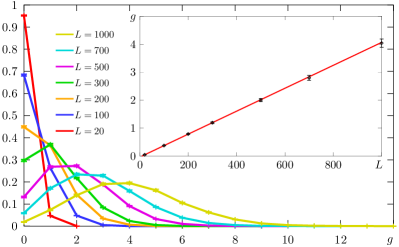
Figure 4: The genus distribution of a two dimensional homopolymer, in the swollen phase $T=10>T^{2D}_{\theta}$, at various values of $L$.

When comparing them with the combinatorial results of PRL , we see that the genus at a fixed $L$ is on the average much smaller. More precisely, below the $\theta$-point the average genus scales like by $\langle g/L\rangle\sim 0.141\pm 0.003$ and $\langle g/L\rangle\sim 0.1318\pm 0.0025$, in $3d$ (at $T=0.2$) and $2d$ (at $T=0.225$), respectively. In both cases the scaling is at a lower rate (about 50% less) than the value $L/4$ computed in PRL . In the swollen-phase (e.g. $T=10>T_{\theta}$), the average genus is given by $\langle g/L\rangle\sim(585\pm 8)10^{-6}$ in $3d$, and $\langle g/L\rangle\sim(410\pm 1)10^{-5}$ in $2d$. Such a low rate comes from the tendency of a homopolymer to develop long rectilinear sub-chains in the swollen phase. In two dimensions the entropic factor is smaller than in three dimensions and the genus growth rate is therefore larger (see Figure 4). Moreover, the genus distributions for $T>T_{\theta}$ are numerically consistent with Poissonian distributions (see Figure 4), whereas at smaller temperatures they are closer to Gaussian ones.

It turns out that the average genus is an extensive quantity, like the energy, and their ratio is shown in Figure 5.

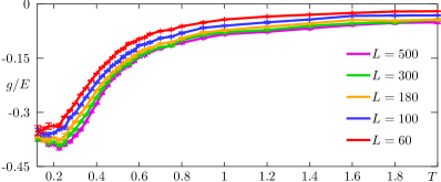
Figure 5: The ratio genus/energy of an homopolymer on a cubic lattice, as a function of $T$, at different values of $L$.

All these results confirm that the genus distribution behaves differently in the two phases, as expected. They also quantify how much the restrictions induced by the actual three-dimensional arrangement of the chain can limit the number and complexity of pseudoknots (compared to PRL ). We find values closer to what seems to happen in pseudoknots of real RNA molecules. In fact, real RNA molecules typically have small genus. For instance, a simple $H$-type pseudoknot ($\sim$20 bases or more) or the classical kissing-hairpins pseudoknot ($\sim$30 bases or more) both have genus 1, much less than the toy-model prediction in PRL . Even tRNAs ($\sim$80 bases) mostly contain 4 helices, two of them linked together by a kissing-hairpin pseudoknot, has still genus 1. Typical tmRNAs ($\sim$350 bases long) contain four $H$-type pseudoknots, and its total genus is 4, far below the theoretical upper bound $L/4$. Our numerical results would instead indicate, for instance for a $80$ bases long homopolymer, a genus of about $11.2$ in three dimensions ($\sim$10.5 in two dimensions). Even if it is smaller than the value suggested in PRL (because of the steric constraints), it is still too high when compared to real RNA molecules. The obvious reasons are that we neither included the primary sequence nor realistic stacking energies. We have nevertheless been able to quantify the general effect of steric constraints on the genus distribution of a pseudoknotted homopolymer on a lattice, as a first step towards a model which includes a more realistic energy function.
Acknowledgements: We wish to thank T. Garel and R. Guida for discussions. This work was supported in part by the National Science Foundation under grant number PHY 99-07949, and by Sonderforschungsbereich-Transregio “Computational Particle Physics” (SFB-TR9). GV acknowledges the support of the European Fellowship MEIF-CT-2003-501547.

References

- (1) R. Schroeder, A. Barta and K. Semrad, Nature Rev. Mol. Cell Biol. 5, 908 (2004).
- (2) I. Tinoco Jr. and C. Bustamante, J. Mol. Biol. 293, 271 (1999).
- (3) P.G. Higgs, Quart. Rev. Biophys. 33, 199 (2000).
- (4) M. Zuker, Nucleic Acids Res. 31, 3406 (2003); See also I.L. Hofacker, Nucleic Acids Research, 31, 3429(2003).
- (5) R.B. Lyngsø and C.N. Pedersen, J. Comput. Biol. 7, 409 (2000).
- (6) C.W. Pleij, K. Rietveld and L. Bosch, Nucleic Acids Res. 11, 1717 (1985).
- (7) L.X. Shen and I. Tinoco Jr, J. Mol. Biol. 247, 963 (1995).
- (8) P.L. Adams, M.R. Stahley, A.B. Kosek, J. Wang and S.A. Strobel, Nature 430, 45 (2004).
- (9) D.W. Staple and S.E. Butcher, PLoS Biol 3, 213 (2005).
- (10) E. Rivas and S.R. Eddy, J. Mol. Biol. 285, 2053 (1999).
- (11) M. Pillsbury, H. Orland and A. Zee, Phys. Rev. E 72, 011911 (2005).
- (12) M. Pillsbury, J.A. Taylor, H. Orland and A. Zee, http:// arXiv.org/cond-mat/0310505.
- (13) A. Xayaphoummine, T. Bucher and H. Isambert, Nucleic Acids Res. 33, 605 (2005).
- (14) A.P. Gultyaev, Nucleic Acids Res. 19, 2489 (1991).
- (15) J.P. Abrahams, M. van den Berg, E. van Batenburg and C.W.A. Pleij, Nucleic Acids Res. 18, 3035 (1990).
- (16) J.E. Tabaska, R. B. Cary, H.N. Gabow and G.D. Stormo, Bioinformatics 14, 691 (1998).
- (17) S.R. Eddy, Nature Biotechnology 22, 1457 (2004).
- (18) H. Orland and A. Zee, Nucl. Phys. B 620, 456 (2002).
- (19) G. ’t Hooft, Nucl. Phys. B 72, 461 (1974).
- (20) G. Vernizzi, H. Orland and A. Zee, http://arxiv.org/q- bio.BM/0405014; see also Acta Phys. Pol. B 36, 2821 and 2829 (2005).
- (21) A. Kabakçioǧlu and A.L. Stella, Phys. Rev. E 70, 011802 (2004).
- (22) E. Rivas and S.R. Eddy, Bioinformatics 16, 334 (2000).
- (23) A. Lucas and K.A. Dill, J. Chem. Phys. 119, 2414 (2003).
- (24) G. Vernizzi, H. Orland and A. Zee, Phys. Rev. Lett. 94 168103 (2005); Virt. J. Biol. Phys. Res. 9, May 1, 2005.
- (25) P.G. De Gennes, Scaling Concepts in Polymer Physics, Cornell University Press (1979); C. Vanderzande,Lattice Models of Polymers, Cambridge University Press (1998).
- (26) T. Garel, H. Orland and E. Orlandini, Eur. Phys. J. B 12, 261-268 (1999).
- (27) D.P. Foster and F. Seno, J. Phys. A 34, 9939 (2001).
- (28) J. Borg, M.H. Jensen, K. Sneppen and G. Tiana, Phys. Rev. Lett. 86, 1031 (2001).
- (29) M. Baiesi, E. Orlandini and A.L. Stella, Phys. Rev Lett. 91, 198102 (2003); P. Leoni and C. Vanderzande, Phys. Rev. E. 68, 051904 (2003).
- (30) T. Garel and H. Orland, J. Phys. A 23, L621 (1990).
- (31) P.G. Higgs and H. Orland, J. Chem. Phys. 95, 4506 (1991).
- (32) Y. Iba, Trans. Jap. Soc. for Artif. Intell. 16, 279 (2001).
- (33) V. Provman, P.C. Hohenberg and A. Aharony, Phase Transitions and Critical Phenomena, edited by C. Domb and J.L Lebowitz, Academic Press, New York (1991).
- (34) B.G. Nickel, Macromolecules 24, 1358 (1991).
- (35) P. Grassberger, Phys. Rev. E 56, 3682 (1997).
- (36) B.Li, N. Madras and A.D. Sokal, J. Stat. Phys. 80, 661 (1995).