Abstract

The distribution of inequivalent geometries occurring during self-assembly of the major capsid protein in thermodynamic equilibrium is determined based on a master equation approach. These results are implemented to characterize the assembly of SV40 virus and to obtain information on the putative pathways controlling the progressive build-up of the SV40 capsid. The experimental testability of the predictions is assessed and an analysis of the geometries of the assembly intermediates on the dominant pathways is used to identify targets for antiviral drug design.

1 Introduction

Manipulating the assembly of viral capsids is one way of interfering with the viral replication cycle and hence a possible avenue for anti-viral drug design. Despite of its importance the theory of viral capsid assembly is still in its infancy. A first model for the self-assembly of a small plant virus was pioneered by Zlotnick [25], exploring the assembly of a dodecagonal shape by a cascade of single order reactions. It has since been extended to more involved scenarios [6, 26, 27], including a study of the energy landscape underlying assembly [7], that is similar to approaches in protein folding [2] or the energy landscape description of association reactions [21, 22, 23]. These results have been used to investigate the possibility of inhibiting assembly via an anti-viral drug in the case of Herpes Virus [28]. Related approaches include molecular dynamics studies of viral capsid assembly [13, 14], and a molecular dynamics-like formalism that is implemented in connection with a “local rules” mechanism that regulates capsid assembly [1, 18].

A characteristic feature of these models is the fact that the bonding structures of all building blocks are treated on an equal footing. While this is justified for a large number of viruses, it is an inappropriate simplification for important families of virus such as the Papovaviridae, which are linked to cancer and are hence of particular interest for the public health sector. For example, the (pseudo-) T=7 capsids in this family are known to be composed of two different types of pentameric building blocks which are distinguished by their local bonding structure. This requires a mathematical representation of these building blocks that takes the differences in the local bonding environments into account. The tiling approach for the description of viral capsids [19, 20] provides an appropriate mathematical framework for this. It encodes the locations of proteins and inter-subunit bonds in terms of tilings, i.e. tessellations that represent the surface structure of the capsids. Since the vertex atlas of these tilings, i.e. the collection of all distinct local configurations around vertices in the tiling, encodes all different types of capsomeres and their bonding structures, it provides appropriate building blocks for the construction of assembly models. An assembly model for (pseudo-) T=7 capsids in the family of Papovaviridae has been introduced along these lines in [10]. In this reference, a tree structure – the assembly tree – has been determined that encodes all energetically preferred pathways of assembly, and it specifies how the tree structure changes in dependence on the association constants. Moreover, the concentrations of the statistically dominant assembly intermediates (i.e. inequivalent shapes at various stages of capsid construction that are located on all pathways) have been computed.

For applications to anti-viral drug design, it is important to control not only the statistically dominant assembly intermediates, but also the concentrations of all other assembly intermediates, and, based on this, to determine the most probable assembly pathway(s). This issue is addressed in this paper, where we adopt a master equation approach for the computation of the concentrations of all assembly intermediates in the assembly tree and use this information to determine the putative pathways controlling the progressive build-up of the capsid. In particular, in section 2 we introduce the master equation approach as a tool for the computation of the concentrations of the assembly intermediates for arbitrary viruses from a thermodynamical point of view. In section 3 we apply this formalism to SV40 virus and determine the equilibrium concentrations of the various assembly intermediates. We discuss how this information can be used to determine the dominant pathway of assembly, and show that the dominant pathways have intermediates with a characteristic structure that may potentially be exploited in the framework of anti-viral drug design. In the final section we summarize our results and assess the implications for other families of viruses.

2 The master equation approach

The formalism presented in this section allows to compute the probability distribution of the inequivalent configurations (also called species or assembly intermediates) that appear during self-assembly of the major capsid protein of a virus in thermodynamic equilibrium. Assume that the different species are indexed from 1 to $N$, where species 1 corresponds to the fundamental building block of the capsid, $N$ to the final capsid, and every other assembly intermediate, $i$, is formed by $n_{i}$ copies of building block 1. As customary, we consider capsid assembly as a sequence of low order reactions, and hence assume that the formation of the capsid occurs from the attachment or detachment of single fundamental units to the partially-formed capsid. From a phenomenological point of view, the equilibrium thermodynamics of the process is described through second-order association constants. Indicating with $[a]$ and $[b]$ the concentrations of two species whose number of constitutive building blocks is, respectively, $n_{a}$ and $n_{b}=n_{a}+1$, we have that their association constant is given by

$$K_{b,a}={[b]_{eq}\over[a]_{eq}[1]_{eq}}\,.$$ (1)

where $[1]$ denotes the concentration of the fundamental building block and the subscripts are used to stress that the concentrations pertaint to the equilibrium (stationary) state. This phenomenological relationship can be related to the fundamental entropic and energetic aspects of the association process through the following factorization (as in [25], [10]):

$$K_{b,a}=\frac{1}{c_{0}}S_{1}\,S_{ba}\,e^{-\Delta G(b,a)\over RT}\,,$$ (2)

where $S_{1}$ denotes the geometric degeneracy of the fundamental “incoming” subunit, $S_{ba}:=O(b)/O(a)$ corresponds to the ratio of the orders of the discrete rotational symmetry groups of the two species $O(b)$ and $O(a)$, $\Delta G(b,a)$ is the free energy difference associated to the bonds formed by the incoming building block, and $R$ and $T$ denote the gas constant ($R=1.987calK^{-1}mol^{-1}$) and, respectively, temperature (chosen as room temperature $T=298K$). The quantity $c_{0}$, having the dimension of a concentration, can be put in unique correspondence with the total concentration of elementary blocks present in the system, as will be shown below.

The hierarchy of association constants of the various pairs of intermediate species differing by one fundamental building block can be used in recursive schemes for obtaining the equilibrium probabilities of any species. In fact, by combining equations (1) and (2) and introducing the adimensional quantity ${\widetilde{[1]}_{eq}}:=\frac{[1]_{eq}}{c_{0}}$ we obtain the fundamental relationship:

$${[b]_{eq}\over[a]_{eq}}=S_{1}\,S_{ba}\,{\widetilde{[1]}_{eq}}\,e^{-\Delta G(b,a)\over RT}$$ (3)

which, used recursively, yields the formal expression of the equilibrium concentration of a generic species, $[i]$, ($i\not=1$),

$$[i]_{eq}=\displaystyle S_{1}^{n_{i}-1}\frac{O(1)}{O(i)}e^{-\frac{\Delta G(i,1)}{RT}}\,[1]_{eq}\,{\widetilde{[1]}_{eq}}^{n_{i}-1},$$ (4)

where $n_{i}$ is the number of fundamental building blocks in species $i$ and $O(1)$ and $O(i)$ refer to the orders of discrete rotational symmetry of subunit $1$ and species $i$, respectively. Notice that equation (4) depends implicitly on $c_{0}$ through $\widetilde{[1]}_{eq}$. This gives the possibility of relating $c_{0}$ to the total concentration of fundamental building blocks, $[c^{*}]$, through the relationship,

$$[c^{*}]=\sum_{i=1}^{N}\,n_{i}\,[i]\ .$$ (5)

Notice that this relationship expresses the law of conservation of the total number of fundamental building blocks present in the system (be they “free” or assembled in intermediate species) and therefore is valid not only in equilibrium. The association constants of equation (1) can be used beyond the equilibrium framework since they constitute the starting point for formulating phenomenological kinetic equations apt to capture the time evolution of the system given the initial concentration of the various species. Within a vanishingly small time interval the concentration of a given species $[i]$ (we assume $i\not=1$) can change only due to the gain or loss of one fundamental building block:

$${d[i]\over dt}=\sum_{m}\,[m]\,W_{m,i}+\sum_{l}\,[l][1]\,W_{l,i}-\sum_{m}\,[i][1]\,W_{i,m}-\sum_{l}\,[i]\,W_{i,l}$$ (6)

where we have omitted the explicit time dependence of the species concentrations. The indices $l$ and $m$ in the sums refer to the species formed by one less, respectively one more, fundamental building block than species $i$. Finally, $W_{i,j}$ denotes the time-independent rate at which transitions are made from configuration $i$ to configuration $j$. The dynamics of the system is thus fully described by the set of coupled equations (6) for each $i\not=1$, supplemented with the conservation law in equation (5). The $W$’s must be appropriately related to the association constants, $K$, to ensure that the correct equilibrium conditions (1) are recovered at large times when the stationary regime is reached (i.e. when $d[i]/dt=0$ for all species $i$).

Among all possible initial conditions for the above mentioned kinetic evolution a particularly appealing and interesting one is represented by the case where the only species being present is the one associated with the fundamental building blocks. At this initial time ($t=0$) the state of the system would then be described as $[1]_{t=0}=[c^{*}]$ and $[j]_{t=0}=0$ for all species $j>1$. The lack of precise experimental characterization of the equilibrium concentrations of the various species in biologically-relevant conditions has lead previous theoretical studies to focus on particularly simple equilibrium situations, namely the one in which the only dominant species are that of the fully-formed capsid and that of the fundamental building blocks; both species are considered as equiprobable so that $[N]_{eq}=[1]_{eq}$ while, for all other species $j$, $[j]_{eq}\approx 0$.

Under these assumptions, the concentration of the fundamental species [1], is therefore expected to take on a rather limited range of values. We build on this observation to simplify the description of the assembly process of equation (6) through a set of effective first order reactions. The key ingredient in our analysis is to modify the right hand side of equation (6) so to neglect the time-dependence of the concentration $[1]$ and absorb it in new effective time-independent transition rates, $W$. It is convenient to recast the kinetics obtained by this simplification of equation (6) not in terms of the concentration of the $i$th species but of the equivalent probability of occurrence, $P_{i}(t)=[i]/\sum_{j}[j]$. The discrete time evolution of $P_{i}$ is therefore governed by the following master equation

$$P_{i}(t+\Delta t)=P_{i}(t)+\Delta t\left(\sum_{j}P_{j}(t)\,W_{j,i}-\sum_{j}P_{i}(t)\,W_{i,j}\right)$$ (7)

where $\Delta t$ is the time step of the discretized evolution (assumed to be sufficiently small to justify the linearization of the continuous time evolution). As before, the only non-zero entries in the transition matrix $W$ are those connecting species which differ by the addition/removal of one fundamental building block. The matrix $W=(W_{i,j})$ has to satisfy a number of properties (see [9]):

• $\Delta t\,\sum_{j}W_{i,j}=1$    (normalization condition) ,

• there exists a finite integer $l$ such that $[W^{l}]_{i,j}>0\ \forall i,j$    (ergodic condition) .

It is easy to check that the first condition ensures that $\sum P_{j}(t)$ is constant at all times while the second one requires that any two configurations must be connected by a finite number of transitions. The above conditions are sufficient to ensure the onset of equilibrium at $t\to\infty$, irrespective of the initial condition of the system. From the stationarity of the equilibrium distribution we obtain, from equation (7) the generalised balance condition:

$$\sum_{j}(P_{j}^{eq}\,W_{j,i}-P_{i}^{eq}\,W_{i,j})=0\ .$$ (8)

The constraints entailed by the balance equation are not sufficient to identify the matrix $W$ uniquely. We solve this ambiguity by adopting the commonly-employed Metropolis criterion within a detailed balance scheme [9]. The detailed balance condition requires that each term in the sum of eqn. (8) is zero. The Metropolis criterion further specifies the precise form of the $W$ matrix elements. Accordingly, for two different species $i$ and $j$, which differ by the addition/removal of one fundamental building block (otherwise $W_{ij}=0$) one has

$$W_{i,j}=\left\{\begin{array}[]{l l}1&\mbox{if $P^{eq}_{i}<P^{eq}_{j}$}\\ P_{j}^{eq}/P_{i}^{eq}&\mbox{otherwise}\end{array}\right.\,.$$ (9)

The diagonal elements are instead obtained from the normalization condition:

$$W_{ii}={1\over\Delta t}-\sum_{j\not=i}\,W_{i,j}\,.$$ (10)

It is easy to check that with this choice of $W$ the equilibrium distribution is stationary under the evolution of equation (7). In the particular context of capsid assembly, the ratio of probabilities in equation (9) is straightforwardly obtained from equation (3) given the proportionality of $[i]$ and $P_{i}$.

Some caveats must be borne in mind when interpreting the outcome of the master equation as a kinetic process. While the equilibrium distribution is insensitive to the choice of the $W$’s, as long as they satisfy equation (8), the kinetics is strongly affected by the form of the $W$ matrix. Our choice follows the common practice of adopting the Metropolis criterion, but remains only one of the equivalent possibilities in terms of correct asymptotic behaviour. Also, we stress again that recasting equation (6) into the master equation of equation (7) was possible upon neglecting the time dependence of [1] in (6).

3 Application of the formalism to SV40 virus

In this section we apply the master equation formalism to the assembly of SV40 virus. The capsid of SV40 is composed of 72 pentameric building blocks that adopt two different types of local configurations (with respect to their local bonding structure) in the capsid. These can be modelled via the tiling approach shown in Fig. 1 adapted from [19].

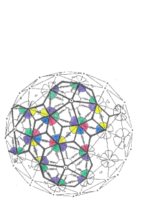
Figure 1: The tiling representing the viral capsid of SV40.

In particular, dimer- and trimer interactions, that is interactions between two, respectively three, protein subunits, are represented geometrically as rhombs, respectively kites. These rhombs and kites (see also Fig. 2) tessellate the surface of the capsid, and encode the locations of the protein subunits and the inter-subunit bonds.

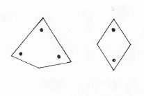
Figure 2: Tiles corresponding to the tiling in Fig. 1.

In particular, tiles have to be interpreted as follows: dots on the tiles correspond to angles of equal magnitude and mark the locations of the protein subunits. The locations of the inter-subunit bonds (C-terminal arm extensions in the case of SV40) correspond to the straight lines connecting these dots.

SV40 has an icosahedrally symmetric capsid, and therefore also the tiling has this symmetry. From the tiling, one can see that the twelve pentamers located at the 5-fold vertices of the capsid are surrounded by trimer-interactions, and the 60 other pentamers by a combination of dimer- and trimer-interactions. There are hence two different types of local environments, which are shown in Fig. 3.

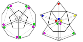
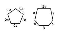
Figure 3: The building blocks for SV40 capsid assembly.

Instead of using the tiles themselves, it is more convenient – and mathematically equivalent – to work with the pentagons and hexagons shown superimposed on the tiles (Fig. 3, left), where the edges of the pentagons and hexagons are labelled according to the association energies related to the tiles they bisect (same figure, right). In particular, for SV40 there are 3 different types of bonds, that correspond to the association energies $a$ for a single C-terminal arm in a kite tile, association energy $b$ for a quasi-dimer bond (”yellow-yellow” rhombs in Fig. 1, named after their location on a local 2-fold symmetry axis), and $c$ for a strict dimer bond (”blue-red” rhombs in the figure, named after their location on a 2-fold symmetry axis). They have to be taken into account when computing the free energies $\Delta G$ in equation 3.

In [10] the assembly of SV40 virus is considered based on these pentagonal and hexagonal building blocks. Assembly is considered as a cascade of low order reactions by association of a single building block at a time. The complete characterization of the assembly thermodynamics would require the full classification of all possible species of correctly-connected pentamers and hexamers, that is all combinatorially possible combinations of these building blocks, even those comprising more than the 72 blocks blocks necessary to form the full capsid (and may correspond to malformed capcids or other types of closed or open structures). Obviously, this exhaustive enumeration cannot be accomplished. Consequently it is necessary to reduce the number of building blocks to a manageable size by discarding configurations that are supposed to play an unimportant role in the assembly process. To illustrate the reduction procedure employed in this study it is convenient to regard the various species as the nodes of a graph. The links in the graph connect species which differ by the attachment/removal of a pentamer of hexamer. The assembly tree containing the species to which we restrict our attention is constructed as follows. Without loss of generality the first node is constituted by the fundamental pentamer. We then consider all the geometrically inequivalent species obtained via the addition of an extra building unit. Of these species we retain only the one (or ones in case of degeneracy) having the lowest free energy. Each of the retained species become new nodes of the graph (and are linked to the parent node). In correspondence of each of these offspring nodes we carry out the search of minimum free-energy descendants, as before. The process ultimately ends when the node corresponding to the full capsid is reached.

Within this limited set of species, the possible assembly pathways are represented as walks on the tree connecting linked nodes. We stress again that, due to the selection criterion based on the free energy minimization, the assembly tree that we obtain represents only a subset of the combinatorially possible nodes. The resulting “minimal tree” is uniquely encoded by the energy parameters, $a,\ b$ and $c$. Since one of these three quantities can be taken as the unit of energy, we have that the choice of the assembly tree depends on two adimensional parameters: $a/c$ and $b/c$. In [10], the phase diagram of the system corresponding to these parameters is depicted. It is shown that one can identify convex regions in this two-dimensional parameter space where parameters can be varied without affecting the assembly tree (but, obviously, the probability of occurrence of the various species will change from point to point in the same region).

While no direct measurement of the association energies $a$, $b$ and $c$ is available, an estimate for the assembly free energies is provided by the VIPER database. We discuss the assembly tree associated with the point $x\equiv b/c\approx 0.92$ and $y\equiv a/c\approx 0.47$, in the phase space, as it corresponds to the ratios of the association energies listed on the VIPER webpages for SV40.

In Fig. 4 we portray the portion of the assembly tree for SV40 limited to species with up to 16 building blocks.

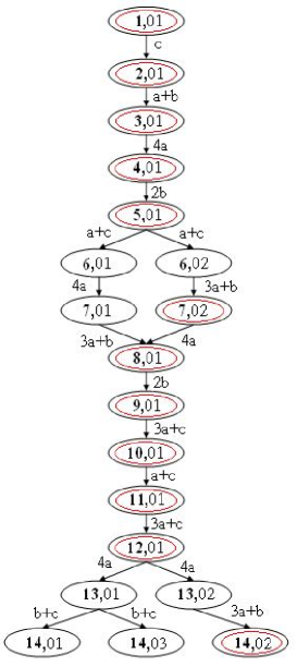
Figure 4: The start of the assembly tree for SV40.

It contains 19 assembly intermediates, out of a total number of 505 assembly intermediates that are encoded by the minimal free-energy assembly tree [10]. The complicated structure of the assembly tree makes impractical the use of relation (4) for computing the relative concentrations of the assembly intermediates. Therefore, only the concentrations of the dominant assembly intermediates, i.e. those located on all paths in the assembly tree such as, for example, the intermediates denoted as 1, 01 to 5, 01 and 8, 01 to 12, 01 in Fig. 4, have been computed prior to this work (see ref. [10]). However, the concentrations of all assembly intermediates are needed in order to obtain clues about the putative pathways of assembly, and hence about possible mechanisms for anti-viral drug design.

To compute the equilibrium probabilities of occupation of the various species, and to identify the dominant kinetic pathway within the assembly tree of Fig. 4 we must go beyond the mere specification of the adimensional parameters $a/c$ and $b/c$ and consider the absolute values of the energies $a,\ b,\ c$. The absolute value of the nominal free energies provided by the VIPER website are more than an order of magnitude larger than the typical interaction energies of biomolecules (usually of the order of a few $Kcal/mol$). The particularly high VIPER values may indeed reflect the shortcoming of the rigid-unit approximations involved in the potential extraction scheme. We shall therefore obtain an indication of the absolute scale for the SV40 free energies and of the concentration $c_{0}$, by following some guidelines inspired by previous theoretical and experimental work.

The first quantitative experimental input pertains to the overall concentration of fundamental units present in solution, $[c^{*}]$, which has, typically, of the order of 10 $\mu$M. Secondly, as anticipated, we wish to describe the situation where the dominant species in equilibrium are $[1]$ and $[N]$ . Assuming that $[N]_{eq}$ and $[1]_{eq}$ are equiprobable one has:

$$1=\frac{[N]_{eq}}{[1]_{eq}}=12\,({{\widetilde{[1]}_{eq}}\over 5})^{71}e^{\kappa\,a/RT}\,,$$ (11)

where $\kappa:=180+60b/a+30c/a\approx 360.8571$.

The above requirement provides a relationship through the free energy scale, $a$, and $c_{0}$ (entering implicitly through $\widetilde{[1]}_{eq})$. The second condition typing $c_{0}$ and $a$ is obtained by requiring that the concentration of species $[2]$ is significantly smaller than $[1]$. This requirement implies, through the chain relations of equation 4, that the dominant species are indeed $[1]$ and $[N]$, so that

$$[c^{*}]=\sum_{k=1}^{505}n_{k}\frac{5^{n_{k}}}{O(k)}e^{-\Delta G(1,k)\over RT}{\widetilde{[1]}_{eq}}^{n_{k}-1}[1]_{eq}\approx[1]_{eq}+72\,[N]_{eq}=73\,[1]_{eq}\ .$$ (12)

We discuss here the case where $[2]=[1]/10$, which is satisfied when $a$ takes on the realistic value, $a\approx-0.7kcal/mol$. All our conclusions about the dominant pathway in the assembly tree are unchanged if much larger values of $a$ (in modulus) are used, although these might result in unrealistically low concentrations of intermediates.

Therefore the assembly tree for SV40 has been computed for the values $a=-0.7$ kcal mol^-1, $b=-1.37$ kcal mol^-1 and $c=-1.49$ kcal mol^-1. The shortest pathways in the tree that connect $[1]$ and $[N]$ (i.e. those without loops) contains precisely 72 species, one for each possible value of building blocks, see Fig. 3.

We have computed the concentrations of the assembly intermediates in thermodynamic equilibrium as shown in Fig. 5.

Figure 5: SV40 capsid assembly: scatter plot for the concentrations of assembly intermediates, $[j]$, as a function of the number of building blocks, $n_{j}$. The concentrations were normalised with respect to that of the fundamental unit, $[1]$. Notice that more than a species may exist for given $n_{j}$. The plot refers to the situation where $[c^{*}]=10\mu$M and $a=-0.7kcal/mol$.

In particular, one observes that concentrations are highest at the beginning and at the end of the assembly pathways, and are strictly and rapidly decreasing (at the beginning) or increasing (at the end). For the intermediates at the start of the assembly tree shown in Fig. 4 one observes furthermore the following scenario: in the cases where more than one intermediate of the same number of building blocks exists (such as for example 6, 01 and 6, 02, or, 7, 01 and 7, 02) their concentrations are either identical as a consequence of degeneracy (such as for 6, 01 and 6, 02 and all other nodes springing out from a parent node), or vary strongly (7, 02 having a larger concentration than 7, 01). In the latter case, we indicate the intermediate with the larger concentration by a double circle in Fig. 4. Our computations show furthermore that for comparable values of probabilities towards the end of the pathways, different intermediates with the same number of building blocks (and hence all assembly pathways) are indistinguishable. Therefore, the start of the assembly pathways singles out the dominant pathway(s). Since dead-ends and traps do not occur in the assembly tree, the pathways containing the two largely dominant configurations 7, 02 and 14, 02 in Fig. 4 must be the dominant pathways during assembly.

The geometries of the intermediates 7, 02 and 14, 02 are shown in Fig. 6.

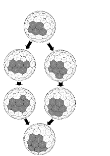
Figure 6: The geometries of the intermediates 7, 02 and 14, 02.

One observes that in each case, the dominant configuration is obtained from the previous intermediate via the formation of bonds with association energy $2a$, $a$ and $b$. The fact that the formation of this constellation of bonds is important is corroborated further by the following: We have increased the association energies of the bonds $a$ and $b$ individually, and have compared the ratio of final capsids to pentamers in equilibrium. In both cases the yield of final capsids has increased, with a stronger increase in response to an increase of the association energy related to the bond with association energy $b$.

These considerations suggest that SV40 capsid assembly is driven more by the details of the association free energies rather than differences in the geometrical entropy associated to rotational symmetries of the various species. This fact can be conveniently checked by setting to zero all association free energies, $a,\ b$ and $c$ and computing the contribution of the factors $S_{1}$ and $S_{n}$ to the concentrations of the various species. One observes that all assembly intermediates (on different assembly pathways) of an equal number of building blocks have the same probability, with the exception of assembly intermediates that have a discrete rotational symmetry. However, since these symmetry corrections appear only at later stages in the pathways (first occurrence at iteration step 30) where concentrations are low when energy effects are counted in, they do not need to be considered when distinguishing the dominant pathways. The dominant pathways are, therefore, strongly dependent on the association free energies.

In [10] it has been shown that the phase space formed by the ratios of the association constants can be partitioned into areas in which the qualitative behaviour of assembly, as encoded in the assembly tree, is indistinguishable. In order to explore if similar results occur also for these other areas in phase space (and hence for different assembly trees), we have calculated the concentrations of the assembly intermediates for a representative of a different area in the partition (area 1 in Fig. 5 [10]). It corresponds to the point $x=0.75$ and $y=0.45$ in phase space. The complete assembly tree consists of 281 species, and the start of the assembly tree is shown in Fig. 7.

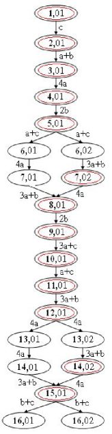
Figure 7: The start of the assembly tree for a representative of a different area in phase space.

The assembly intermediates with the larger concentrations are again marked by double circles. As in the case of SV40 assembly, the occurrence of assembly intermediates with concentrations larger that that of the other intermediates with the same number of building blocks is related to the formation of bonds with association energies $2a$, $a$ and $b$. This phenomenon hence seems pertinent to the selection of the dominant pathways, and may therefore provide insight into the aspect of the viral assembly which may become target of drugs.

4 Discussion

We have demonstrated that a combination of the master equation and the tiling approach allows to determine the putative pathways for SV40 capsid assembly and sheds light on the mechanisms that drive capsid assembly. In particular, we have demonstrated that the more important assembly pathways are those where a particular constellation of bonds is formed at an early stage (see Fig. 6). Hence, this constellation of bonds could be a possible target for antiviral drug design; for example, it suggests to search for a drug that binds to the sites related to these bonds, hence preventing the formation of this particular constellation of bonds.

Moreover, our analysis has shown that SV40 capsid assembly is strongly driven by the details of the association free energies of the tiles and is only slighted affected by the entropic aspects associated to the different rotational symmetries of the various species. While this may be similar for other DNA viruses, it is presumably not the case for RNA viruses due to the interactions between RNA and the protein building blocks of the capsids. This fact justifies to neglect other combinatorially possible intermediates, which however may be important for other viruses as demonstrated in [7].

References

- [1] Berger, B. et al. (1994), Proc. Natl. Acad. Sci. 91, pp. 7732.
- [2] Brooks III, C.L. et al. (1998), Proc. Natl. Acad. Sci. 95, pp. 11037.
- [3] Casjens, S. (1985). Virus structure and assembly. Jones and Bartlett, Boston, Massachusets.
- [4] Johnson, J.M. et al. (2005) - Nanoletters - complete…
- [5] Caspar, D.L.D. and A. Klug (1962), Cold Spring Harbor Symp. Quant. Biol. 27, pp. 1.
- [6] Endres, D. and A. Zlotnick (2002), Biophysical Journal 83, pp. 1217.
- [7] Endres, D., Miyahara, M., Moisant, P. and A. Zlotnick (2005), Protein Science 14, pp. 1518.
- [8] Horton, N. and M. Lewis (1992), Protein Science 1, pp. 169.
- [9] Itzykson & Drouffe, Statistical field theory, 2nd volume
- [10] Keef, T., Taormina, A. and Twarock, R. (2005) Assembly Models for Papovaviridae based on Tiling Theory, submitted to J. Phys. Biol..
- [11] Liddington, R.C. et al. (1991), Nature 354, pp. 278.
- [12] Modis, Y., et al. (2002), EMBO J. 21, pp. 4754.
- [13] Rapaport, D.C., et al. (1999), Comp. Phys. Comm. 121, pp. 231.
- [14] Rapaport, D.C., et al. (2004), Phys. Rev. E 70, pp.
- [15] Rayment, I., et al. (1982), Nature 295, pp. 110.
- [16] Reddy, V. S. et al. (1998), Biophysical Journal 74, pp. 546.
- [17] Reddy, V. S. et al. (2001). J. Virol. 75 pp. 11943.
-
[18]
Schwartz, R. et al. (1998). Biophys. J. 75 pp. 2626.
Schwartz, R. et al. (2000). Virology 268 pp. 461. - [19] Twarock, R. (2004), J. Theor. Biol. 226, pp. 477.
- [20] Twarock, R. (2005), Bull. Math. Biol. 68, in press.
- [21] Wales, D.J. (1987), Chem. Phys. Lett. 141, pp. 478.
- [22] Wales, D.J. (1996), Science 271, pp. 925.
- [23] Wolynes, P.G. (1996), Proc. Natl. Acad. Sci. 93, pp. 14249.
- [24] Zandi, R. et al. (2004), Proc. Natl. Acad. Sci. 101, pp. 15556.
- [25] Zlotnick, A. (1994), J. Mol. Biol., 241, pp. 59.
- [26] Zlotnick, A. et al., (1999), Biochemistry, 38, pp. 14644.
- [27] Zlotnick, A. et al., (2000), Virology, 277, pp. 450.
- [28] Zlotnick, A. et al., (2002), J. Virol., 76, pp. 4848.