Signal detection, modularity and the correlation between extrinsic and intrinsic noise in biochemical networks

Abstract

Understanding cell function requires an accurate description of how noise is transmitted through biochemical networks. We present an analytical result for the power spectrum of the output signal of a biochemical network that takes into account the correlations between the noise in the input signal (the extrinsic noise) and the noise in the reactions that constitute the network (the intrinsic noise). These correlations arise from the fact that the reactions by which biochemical signals are detected necessarily affect the signaling molecules and the detection components of the network simultaneously. We show that anti-correlation between the extrinsic and intrinsic noise enhances the robustness of zero-order ultrasensitive networks to biochemical noise. We discuss the consequences of the correlation between extrinsic and intrinsic noise for a modular description of noise transmission through large biochemical networks in the context of the mitogen-activated protein kinase cascade.

Living cells process information in a stochastic manner  McAdams and Arkin (1997); Elowitz and Leibler (2000); Ozbudak et al. (2002); Elowitz et al. (2002); Ozbudak et al. (2004); Pedraza and van Oudenaarden (2005); Rosenfeld et al. (2005); Blake et al. (2003); Raser and O’Shea (2004); Acar et al. (2005); Becksei et al. (2005); Colman-Lerner et al. (2005); Korobkova et al. (2004). It it generally believed that biochemical noise can be detrimental to cell function, because it can hamper the reliable integration and transmission of signals Rao et al. (2002). It is increasingly becoming recognized, however, that stochasticity can also play a beneficial role Kaern et al. (2005). Biochemical noise can enhance the functioning of biochemical networks by, e.g., increasing the sensitivity Paulsson et al. (2000) or by driving oscillations Vilar et al. (2002), while stochastic switching between phenotypes can increase the proliferation of an organism in a randomly fluctuating environment Thattai and van Oudenaarden (2004); Kussell and Leibler (2005). It is thus important to understand how living cells process noisy signals. The complete biochemical network of a living cell consists of a huge number of biochemical reactions. This precludes a detailed mesoscopic description of the propagation of noise through the full network. However, it is believed that biochemical networks are modular in design, which means that they can be decomposed into smaller, functionally independent units Hartwell et al. (1999); Kashtan and Alon (2005). This is potentially useful, because it would make it possible to coarse-grain the full network of individual reactions to a smaller network consisting of modules, where each module is described as a ‘black box’ with input and output signals; the reactions that constitute each module would then be integrated into the input-output relations Angeli et al. (2004). This would allow a simplified description of the behavior of the full network Hartwell et al. (1999); Angeli et al. (2004). It is not clear, however, whether such a description is possible for the transmission of noise. Here we address the question: under which conditions can modularity be exploited to develop a coarse-grained description for the transmission of noise?

Recently, several groups have derived analytical expressions for the noise in the output signal of a network as a function of the noise in the input signal, known as the “extrinsic noise”, and the noise in the biochemical reactions that constitute the network, the “intrinsic noise” Detwiler et al. (2000); Thattai and van Oudenaarden (2002); Paulsson (2004); Shibata and Fujimoto (2005). These results suggest that the input-output relations for the noise of the individual modules of a network can be combined in a simple way to quantify the transmission of noise through the full network Detwiler et al. (2000); Thattai and van Oudenaarden (2002); Shibata and Fujimoto (2005). However, these studies assume that the extrinsic and intrinsic noise are independent sources of noise Detwiler et al. (2000); Thattai and van Oudenaarden (2002); Paulsson (2004); Shibata and Fujimoto (2005). Here, we show that the biochemical reactions that allow a module to detect the incoming signals introduce correlations between the fluctuations in the input signals and the intrinsic noise of the processing module; the extrinsic and intrinsic noise are not therefore independent of one another. This means that the fluctuations in the output signal of one module (which depend upon the intrinsic noise of that module) can affect the intrinsic noise of another module. As a consequence, the modules do not perform independently of one another and this, in general, impedes a quantitative modular description of the propagation of noise through large scale biochemical networks. Our analysis also reveals the conditions under which detection reactions do not introduce correlations between the extrinsic and intrinsic noise; under these conditions, a modular description of noise transmission can be developed.

We study the consequences of the correlations between extrinsic and intrinsic noise for the mechanism of zero-order ultrasensitivity Goldbeter and Koshland, Jr. (1981). Zero-order ultrasensitivity is one of the principal mechanisms that allow cells to strongly amplify input signals Goldbeter and Koshland, Jr. (1981); Ferrell, Jr. (1996). It operates in push-pull networks, which are ubiquitous in prokaryotes and eukaryotes. In a push-pull network, two enzymes covalently modify a component in an antagonistic manner, e.g., a kinase that phosphorylates a component and a phosphatase that dephosphorylates the same component (see Fig. 1). If both enzymes operate near saturation, then the modification and demodification reactions will be zero-order, which means that their reaction rates become insensitive to the substrate concentrations. Under these conditions, a small change in the concentration of one of the two enzymes, will lead to a large change in the concentration of the modified protein. Zero-order ultrasensitivity thus allows push-pull networks to turn a graded input signal (the concentration of one the enzymes) into a nearly binary output signal (the covalently modified protein) Goldbeter and Koshland, Jr. (1981); Ferrell, Jr. (1996). However, if the enzymes operate near saturation, then these networks are also known to exhibit large intrinsic fluctuations Berg et al. (2000). This will not only weaken the sharpness of the macroscopic response curve Berg et al. (2000), but will also strongly limit the detectability of the input signal Detwiler et al. (2000). Moreover, large extrinsic fluctuations in, e.g., the activity of the kinase, can induce bistability in the network Samoilov et al. (2005). In order to understand the performance of zero-order ultrasensitive networks, it is therefore important to understand not only their macroscopic input-output curves, but also their noise characteristics.

Figure 1: The Mos/MEK/p42 MAPK cascade. This network consists of three tiers, which, from a topological point of view, could be regarded as modules. Note also that the full network consists of push-pull networks, in which the activity of an enzyme is covalently modified by the action of two opposing enzymes.

The noise properties of zero-order ultrasensitive networks have been studied extensively Detwiler et al. (2000); Berg et al. (2000); Shibata and Fujimoto (2005); Samoilov et al. (2005). However, all these studies have ignored the correlations between the extrinsic and intrinsic noise: the modification and demodification reactions were assumed to be given by Michaelis-Mention kinetics without explicitly taking into account the binding and unbinding of the enzymes to their substrates Detwiler et al. (2000); Berg et al. (2000); Shibata and Fujimoto (2005); Samoilov et al. (2005). Here, we show that the (un)binding of the enzymes to their substrates induces anti-correlations between the extrinsic noise – the fluctuations in the activating enzyme – and the intrinsic noise – the fluctuations in the modification and demodification reactions. These anti-correlated fluctuations reduce the noise in the output signal (the covalently modified protein). While it has long been known that temporal fluctuations in the network components can adversely affect the performance of zero-order ultrasensitive networks Rao et al. (2002); Berg et al. (2000), our calculations reveal that anti-correlated fluctuations between different sources of noise can, in fact, enhance their performance by increasing the signal-to-noise ratio.

Finally, we illustrate the consequences of the correlations between extrinsic and intrinsic noise for a modular description of noise propagation using the MAPK cascade. This network is an important intracellular signaling pathway in eukaryotes, where it plays a central role in cell proliferation, cell differentiation, and cell cycle control Ferrell, Jr. (1996). The MAPK cascade consists of three push-pull modules connected in series (see Fig. 1). We find that because of the correlations, the modules no longer perform independently of one another. As a result, an iterative application of noise-input-output relations of the individual modules drastically overestimates the propagation of noise. Only by analyzing the modules together at the level of the individual biochemical reactions do we arrive at the correct result.

The noise properties of genetic networks in both prokaryotes Elowitz and Leibler (2000); Ozbudak et al. (2002); Elowitz et al. (2002); Pedraza and van Oudenaarden (2005); Rosenfeld et al. (2005) and eukaryotes Blake et al. (2003); Raser and O’Shea (2004); Acar et al. (2005); Becksei et al. (2005); Colman-Lerner et al. (2005) have been measured. While noise in signaling pathways has been studied to some extent in prokaryotes Korobkova et al. (2004), noise in eukaryotic signaling networks has not yet been experimentally investigated. Our results provide a general, quantitative framework for describing the transmission of noise in gene regulatory networks and signal transduction pathways.

I Noise addition rule: uncorrelated extrinsic and intrinsic noise

We consider a module with one input and one output signal. We imagine that the module is a ‘black box’: we will not therefore consider the biochemical reactions that constitute the module explicitly. Clearly, in general, the incoming signal could be transformed into the outgoing signal in a complicated manner, depending upon the reactions that form the module. We imagine, however, that the system is in steady state and we assume that the fluctuations of the incoming and outgoing signals around their steady-states values are small; this allows us to linearize the coupling between them and to use the linear-noise approximation van Kampen (1992). Moreover, we will here assume that the noise in the input and output signals is uncorrelated and that the output signal relaxes exponentially with decay rate $\mu$. This yields the following chemical Langevin equation for the output signal

$$\dot{x}=\nu s(t)-\mu x+\eta(t).$$ (1)

Here, $s=S-\langle{S}\rangle$ is the deviation of the number of signaling molecules, $S$, from its mean, $\langle{S}\rangle$, and $x=X-\langle{X}\rangle$ is the corresponding quantity for the output signal; $\nu$ corresponds to the differential gain and the dot denotes a time derivative. The last term, $\eta(t)$, describes the fluctuations in the reactions that constitute the processing unit; we repeat that we make the crucial assumption that this is uncorrelated from the input signal $s(t)$. We model $\eta(t)$ as Gaussian white noise: $\langle{\eta(t)}\rangle=0$ and $\langle{\eta(t)\eta(t^{\prime})}\rangle=\sigma_{\eta}^{2}\delta(t-t^{\prime})$. By taking the Fourier transform we obtain the power spectrum $S_{{\mathrm{X}}}$ for the the outgoing signal:

$$S_{{\mathrm{X}}}(\omega)=\langle{|\tilde{x}(\omega)|^{2}}\rangle=\frac{2\,\sigma_{\mathrm{in}}^{2}\mu}{\nu^{2}+\omega^{2}}+\frac{\nu^{2}}{\mu^{2}+\omega^{2}}S_{{\mathrm{S}}}(\omega),$$ (2)

where $\sigma_{\mathrm{in}}^{2}=\sigma_{\eta}^{2}/(2\mu)$ is the intrinsic noise and $S_{{\mathrm{S}}}(\omega)=\langle{|\tilde{s}(\omega)|^{2}}\rangle$ is the power spectrum of the incoming signal. A similar expression has been obtained recently Detwiler et al. (2000); Simpson et al. (2004); Shibata and Fujimoto (2005). We refer to Eq. 2 as the spectral addition rule.

Eq. 2 has the attractive interpretation that the computational module acts as a low-pass filter for the input noise (second term) and generates its own noise in the process (first term); the filter function $\nu^{2}/(\mu^{2}+\omega^{2})$ filters the high-frequency components in the input signal. Moreover, in this model, the effects are additive: the intrinsic noise is simply that which would arise if the input signal did not fluctuate; conversely, the extrinsic noise is not affected by the intrinsic noise. The spectral addition rule is a consequence of the linear response of $x$ to the sum $\nu s(t)+\eta(t)$ (Eq. 1), and the assumption that $s(t)$ and $\eta(t)$ are uncorrelated.

If the autocorrelation function for the noise in the incoming signal has an amplitude $\sigma_{\mathrm{s}}^{2}$ and decays exponentially with a relaxation rate $\lambda$, then its power spectrum is given by

$$S_{{\mathrm{S}}}(\omega)=\frac{2\,\sigma_{\mathrm{s}}^{2}\lambda}{\lambda^{2}+\omega^{2}}.$$ (3)

In this case, the total noise in the outgoing signal, $\sigma_{\mathrm{tot}}^{2}=1/(2\pi)\int_{-\infty}^{\infty}d\omega\,S_{{\mathrm{X}}}(\omega)$, is given by

$$\sigma_{\mathrm{tot}}^{2}=\sigma_{\mathrm{in}}^{2}+g^{2}\frac{\langle{X}\rangle^{2}}{\langle{S}\rangle^{2}}\frac{\mu}{\lambda+\mu}\,\sigma_{\mathrm{s}}^{2}\equiv\sigma_{\mathrm{in}}^{2}+\sigma_{\mathrm{ex}}^{2}.$$ (4)

Here, $\sigma^{2}_{\mathrm{ex}}$ is the extrinsic noise and $g\equiv\partial\ln\langle{X}\rangle/\partial\ln\langle{S}\rangle=(\nu/\mu)\,\,\langle{S}\rangle/\langle{X}\rangle$ is the logarithmic gain. This relation has been derived recently by Paulsson Paulsson (2004) and Shibata and Fujimoto Shibata and Fujimoto (2005). We refer to Eq. 4 as the noise addition rule. It is only valid if the incoming signal has a single exponential relaxation time and if the spectral addition rule, Eq. 2, holds, which means that the incoming signal and the intrinsic noise must be uncorrelated.

Eqs. 2 and 4 are potentially powerful relations, because they allow a modular description of noise propagation. If, for instance, the network consists of a number of modules connected in series, then, once the intrinsic noise for each of the individual modules is known, the propagation of noise through the network can be obtained for arbitrarily varying input signals by the recursive application of the spectral addition rule, Eq. 2, to the successive modules Detwiler et al. (2000); Thattai and van Oudenaarden (2002); the noise strength of the output signal of the network could then be obtained by integrating over its power spectrum. However, this approach requires that the spectral addition rule holds for each of the individual modules. Below, we will show that the detection reactions can introduce correlations between the extrinsic and intrinsic noise. These correlations lead to a break down of the spectral addition rule, impeding a quantitative modular description of the transmission of noise through large networks.

II Correlated extrinsic and intrinsic noise

To elucidate the origin of the correlations between the extrinsic and intrinsic noise, it will be instructive to consider a module that consists of one component only. This component, $\mathrm{X}$, both detects the input signal $\mathrm{S}$ and provides the output signal. In the next section we will generalize our results and discuss more complex modules. To capture the correlations between the extrinsic and intrinsic noise, we explicitly describe the detection of the signal by studying the coupled Langevin equations for the two interacting species – the signaling molecules $\mathrm{S}$ and the detection molecules $\mathrm{X}$; only by analyzing the input signal and the processing module together, do we arrive at the correct results.

	Scheme	Examples
(I)	${\mathrm{S}}+{\mathrm{W}}\overset{\nu=k_{f}{\mathrm{W}}}{\underset{\mu}{\rightleftarrows}}{\mathrm{X}}$
(II)	${\mathrm{S}}\stackrel{{\scriptstyle\nu}}{{\longrightarrow}}{\mathrm{X}}\stackrel{{\scriptstyle\mu}}{{\longrightarrow}}{\emptyset}$
(III)	${\mathrm{S}}\stackrel{{\scriptstyle\nu}}{{\longrightarrow}}{\mathrm{S}}+{\mathrm{X}}$,  ${\mathrm{X}}\stackrel{{\scriptstyle\mu}}{{\longrightarrow}}{\emptyset}$

Table 1: Three elementary detection motifs. Here, ${\mathrm{X}}$ is the output signal and ${\mathrm{S}}$ is the input signal; in motif I, ${\mathrm{W}}$ is the inactive (unbound) state of the detection component and ${\mathrm{X}}$ the active (bound) state. All these schemes have ${\emptyset}\overset{k}{\longrightarrow}n\,{\mathrm{S}}$ and ${\mathrm{S}}\overset{\lambda}{\longrightarrow}{\emptyset}$ as a precursor to generate an input signal which fluctuates about a steady state. For all the schemes, the mean output signal obeys $d\langle{X}\rangle/dt=\nu\langle{S}\rangle-\mu\langle{X}\rangle$. A class of examples of detection motif II is the endocytosis of receptors such as the EGF receptors, which, upon ligand binding, are endocytosed together with the ligand Felder et al. (1992).

The most general form of the two coupled chemical Langevin equations is

$$\dot{s} =-\lambda s+\kappa x+\xi(t),$$ (5a)

$$\dot{x} =\nu s-\mu x+\eta(t).$$ (5b)

Here, $$\kappa \xi(t) s \xi(t) \eta(t) \langle{\xi(t)}\rangle=\langle{\eta(t)}\rangle=0 \langle{\xi(t)\xi(t^{\prime})}\rangle=\langle{\xi^{2}}\rangle\delta(t-t^{\prime}) \langle{\eta(t)\eta(t^{\prime})}\rangle=\langle{\eta^{2}}\rangle\delta(t-t^{\prime}) \langle{\xi(t)\eta(t^{\prime})}\rangle=\langle{\xi\eta}\rangle\delta(t-t^{\prime}) S_{{\mathrm{S}}}(\omega) S_{{\mathrm{X}}}(\omega)$$ describes how the number of signaling molecules is directly affected by the number of (active) detection molecules and models the noise in ; the noise terms, and , are modeled as correlated Gaussian white noise: , , and . The pair of linear differential equations in Eq. 5 can be solved using Fourier transformation, which leads to the following power spectra for the signaling molecules, , and detection molecules, ,

$$S_{{\mathrm{S}}}(\omega) ={\frac{{\kappa^{2}}\,{\langle{\eta^{2}}\rangle}+2\,\kappa\,\mu\,\langle{\xi\eta}\rangle+\left({\mu^{2}}+{{\omega}^{2}}\right)\,{\langle{\xi^{2}}\rangle}}{{{\left(\kappa\,\nu-\lambda\,\mu\right)}^{2}}+\left({\lambda^{2}}+2\,\kappa\,\nu+{\mu^{2}}\right)\,{{\omega}^{2}}+{{\omega}^{4}}}},$$ (6a)

$$S_{{\mathrm{X}}}(\omega) ={\frac{\langle{\eta^{2}}\rangle\,\left({\lambda^{2}}+{{\omega}^{2}}\right)+2\,\lambda\,\nu\,\langle{\xi\eta}\rangle+{\nu^{2}}\,\langle{\xi^{2}}\rangle}{{{\left(\kappa\,\nu-\lambda\,\mu\right)}^{2}}+\left({\lambda^{2}}+2\,\kappa\,\nu+{\mu^{2}}\right)\,{{\omega}^{2}}+{{\omega}^{4}}}}.$$ (6b)

In contrast to Eq. 2, Eq. 6 takes into account the correlation between the noise in the external signal and the intrinsic noise of the processing unit. Importantly, if both $\kappa$ and $\langle{\xi\eta}\rangle$ are zero, then Eq. 6 reduces to Eq. 2.

The correlations between extrinsic and intrinsic noise can have two distinct origins. Both are a consequence of the molecular character of the components; the correlations are thus unique to biochemical networks and absent in electronic circuits. We will illustrate the sources of correlations using three elementary detection motifs, which are described in Table 1; Table 2 shows their power spectra and noise strengths. The motifs obey the same macroscopic chemical rate equation and have the same intrinsic noise. However, the noise in the input signals is transmitted differently. The differences between the motifs are due to the different sources of correlations that are present.

The first source of correlation between the extrinsic and intrinsic noise arises from the fact that the processing unit can act back on the input signal by directly affecting the number of signaling molecules; this corresponds to a non-zero value of $\kappa$. This source of correlation is present in detection motif I, where it arises from the unbinding of signaling molecules from the detection molecules. For scheme I, $\kappa=\mu$; the effect of this source of correlation on the noise in $\mathrm{S}$ and $\mathrm{X}$ depends upon the values of all the rate constants (see Eq. 6) and can either be negative or positive. The second possible source of correlation between the extrinsic and intrinsic noise is the correlated fluctuations in the number of signaling molecules and detection molecules, which arise from detection reactions that simultaneously change the number of both species; these correlated fluctuations are quantified via the cross-correlation function $\langle{\xi(t)\,\eta(t^{\prime})}\rangle$. This source of correlation is present in both schemes I and II, since each time a detection reaction fires, a signaling molecule is consumed and simultaneously a molecule of the processing module is produced (or activated). Additionally, for scheme I, the unbinding reactions also lead to cross-correlations in $\xi(t)$ and $\eta(t)$. For scheme I, $\langle{\xi\eta}\rangle=-(\nu\langle{S}\rangle+\mu\langle{X}\rangle)$, while for scheme II, $\langle{\xi\eta}\rangle=-\nu\langle{S}\rangle$ Gillespie (2000). We emphasize that the sign of $\langle{\xi\eta}\rangle$ is negative; the extrinsic and intrinsic noise are thus anti-correlated. Eq. 6 shows that these anti-correlated fluctuations can lower the noise in $\mathrm{S}$ and $\mathrm{X}$.

Scheme	Noise strength	Noise power spectrum
(I)	$\begin{array}[]{l}\displaystyle{\sigma_{\mathrm{s}}^{2}=\langle{S}\rangle\,\frac{(n+1)(\lambda+\mu)+2\nu}{2(\lambda+\mu+\nu)}}\\[12.0pt] \displaystyle{\sigma_{\mathrm{x}}^{2}=\sigma_{\mathrm{in}}^{2}+g^{2}\frac{\langle{X}\rangle^{2}}{\langle{S}\rangle^{2}}\frac{(n-1)\mu}{(n+1)(\lambda+\mu)+2\nu}\,\sigma_{\mathrm{s}}^{2}}\end{array}$	$\begin{array}[]{l}\displaystyle{S_{\mathrm{s}}(\omega)=\langle{S}\rangle\,\frac{(n+1)\mu^{2}\lambda+(2\nu+(n+1)\lambda)\omega^{2}}{\mu^{2}\lambda^{2}+(\lambda^{2}+\mu^{2}+\nu^{2}+2\nu(\lambda+\mu))\omega^{2}+\omega^{4}}}\\[12.0pt] \displaystyle{S_{\mathrm{x}}(\omega)=\langle{X}\rangle\,\frac{\mu[\lambda(2\lambda+(n+1)\nu)+2\omega^{2}]}{\mu^{2}\lambda^{2}+(\lambda^{2}+\mu^{2}+\nu^{2}+2\nu(\lambda+\mu))\omega^{2}+\omega^{4}}}\end{array}$
(II)	$\begin{array}[]{l}\displaystyle{\sigma_{\mathrm{s}}^{2}=\langle{S}\rangle\,\frac{n+1}{2}}\\[12.0pt] \displaystyle{\sigma_{\mathrm{x}}^{2}=\sigma_{\mathrm{in}}^{2}+g^{2}\frac{\langle{X}\rangle^{2}}{\langle{S}\rangle^{2}}\frac{(n-1)\mu}{(n+1)(\lambda+\mu+\nu)}\,\sigma_{\mathrm{s}}^{2}}\end{array}$	$\begin{array}[]{l}\displaystyle{S_{\mathrm{s}}(\omega)=\langle{S}\rangle\,\frac{(n+1)(\lambda+\nu)}{(\lambda+\nu)^{2}+\omega^{2}}}\\[12.0pt] \displaystyle{S_{\mathrm{x}}(\omega)=\frac{2\sigma_{\mathrm{in}}^{2}\mu}{\mu^{2}+\omega^{2}}+\frac{\nu^{2}}{\mu^{2}+\omega^{2}}\,\frac{n-1}{n+1}\,S_{{\mathrm{S}}}(\omega)}\end{array}$
(III)	$\begin{array}[]{l}\displaystyle{\sigma_{\mathrm{s}}^{2}=\langle{S}\rangle\,\frac{n+1}{2}}\\[12.0pt] \displaystyle{\sigma_{\mathrm{x}}^{2}=\sigma_{\mathrm{in}}^{2}+g^{2}\frac{\langle{X}\rangle^{2}}{\langle{S}\rangle^{2}}\frac{\mu}{\lambda+\mu}\,\sigma_{\mathrm{s}}^{2}}\end{array}$	$\begin{array}[]{l}\displaystyle{S_{\mathrm{s}}(\omega)=\langle{S}\rangle\,\frac{(n+1)\lambda}{\lambda^{2}+\omega^{2}}}\\[12.0pt] \displaystyle{S_{\mathrm{x}}(\omega)=\frac{2\sigma_{\mathrm{in}}^{2}\mu}{\mu^{2}+\omega^{2}}+\frac{\nu^{2}}{\mu^{2}+\omega^{2}}\,S_{{\mathrm{S}}}(\omega)}\end{array}$

Table 2: Exact solutions for the noise strengths and the noise power spectra, for the three detection motifs shown in Table 1; in scheme I, the detection molecules $W$ are assumed to be present in abundance. The noise strengths $\sigma_{\mathrm{s}}^{2}$ and $\sigma_{\mathrm{x}}^{2}$ correspond to the noise strengths of the input and output signal, respectively, and $S_{{\mathrm{S}}}(\omega)$ and $S_{{\mathrm{X}}}(\omega)$ denote the respective power spectra. For all motifs, the intrinsic noise is $\sigma_{\mathrm{in}}^{2}=\langle{X}\rangle$ and the logarithmic gain $g=\partial\ln\langle{X}\rangle\,/\,\partial\ln\langle{S}\rangle=(\nu/\mu)\,\,\langle{S}\rangle/\langle{X}\rangle$. Only scheme III obeys the spectral and noise addition rules (see Eqs. 2 and 4).

For detection motif III, both $\kappa$ and $\langle{\xi\eta}\rangle$ are zero. This scheme is the only one for which there is no correlation between the extrinsic and intrinsic noise. In motif III, the incoming signal catalyzes the activation of detection molecules. This reaction does not affect the signal in any way. The extrinsic and intrinsic noise are therefore uncorrelated and the spectral addition rule, Eq. 2, holds. In this example the input signal relaxes mono-exponentially, so that the noise addition rule, Eq. 4, also holds.

III General processing modules and modular description of noise transmission

The systems discussed in the previous section consist of one component only. In appendix B, we derive the power spectra of the output signals of modules that consist of an arbitrary number of linear(ized) reactions; they are a generalization of Eq. 6. Here, we summarize the main results and discuss how correlations between extrinsic and intrinsic noise affect a modular description of noise transmission through large networks.

If the incoming signals of a module are uncorrelated with each other and are processed via detection scheme III, then the power spectrum of the outgoing signal ${\mathrm{X}}_{i}$ is given by

$$S_{{\mathrm{X}}_{i}}(\omega)=S^{\mathrm{in}}_{{\mathrm{X}}_{i}}(\omega)+\sum_{j}\tilde{g}_{\mathrm{X}_{i}}^{\mathrm{S}_{j}}(\omega)S_{\mathrm{S}_{j}}(\omega).$$ (7)

The first term on the right-hand side is the power spectrum of the intrinsic noise in ${\mathrm{X}}_{i}$ and $\tilde{g}_{\mathrm{X}_{i}}^{\mathrm{S}_{j}}(\omega)$ is the frequency dependent gain corresponding to input signal $\mathrm{S}_{j}$. The gain $\tilde{g}_{\mathrm{X}_{i}}^{\mathrm{S}_{j}}(\omega)$ is determined by the coupling between the network components (see appendix B), which, in general, relax multi-exponentially. A noise addition rule analogous to Eq. 4 is therefore no longer obeyed. A spectral addition rule, Eq. 7, nevertheless still holds for these modules, because the extrinsic and intrinsic noise are independent of one another – the input signals are detected via motif III. Accordingly, the extrinsic contributions to the power spectrum of the output signal can be factorized into a function that only depends upon the intrinsic properties of the module, namely $\tilde{g}_{\mathrm{X}_{i}}^{\mathrm{S}_{j}}(\omega)$, and one that only depends upon the input signal, $S_{\mathrm{S}_{j}}(\omega)$. This allows a simple and modular description of noise transmission.

If a module receives its input via detection scheme I or II, then correlations will be induced between the noise in the input signals and the intrinsic noise of the module. In this case, the spectral addition rule, Eq. 7, and hence the noise addition rule Paulsson (2004); Shibata and Fujimoto (2005) break down. More importantly, the correlations mean that the noise in the output signal of one module (which depends upon the intrinsic noise of that module) affects the intrinsic noise of another module. As a result, the intrinsic fluctuations of the different modules become correlated with one another; the modules therefore no longer perform independently of one another. This precludes a modular description of noise propagation, because the modules have to be analyzed together at the mesoscopic level of the individual biochemical reactions.

IV Zero-order ultrasensitivity

We illustrate the consequences of correlated extrinsic and intrinsic noise using the following push-pull network (see also Fig. 1):

$${\mathrm{E_{a}}}+{\mathrm{W}}\overset{a_{1}}{\underset{d_{1}}{\rightleftarrows}}{\ \mathrm{E_{a}W}}\overset{k_{1}}{\longrightarrow}{\mathrm{E_{a}}}+{\mathrm{X}}$$ (8a)

$${\mathrm{E_{d}}}+{\mathrm{X}}\overset{a_{2}}{\underset{d_{2}}{\rightleftarrows}}{\ \mathrm{E_{d}X}}\overset{k_{2}}{\longrightarrow}{\mathrm{E_{d}}}+{\mathrm{W}}$$ (8b)

Here, ${\mathrm{E_{a}}}$ is the activating enzyme that provides the incoming signal and ${\mathrm{E_{d}}}$ is the deactivating enzyme; the substrate ${\ \mathrm{W}}$ is the unmodified component that serves as the detection component and ${\mathrm{X}}$ is the modified component that provides the outgoing signal.

We have computed the noise in the output signal ${\rm X}$ for the push-pull network of Eq. 8. The input signal ${\rm E_{a}}$ is modeled as a birth-death process, corresponding to (de)activation of ${\rm E_{a}}$. The analysis has been performed using the linear-noise approximation van Kampen (1992) (see Appendix C) and its accuracy was verified by performing kinetic Monte Carlo simulations of the chemical master equation Bortz et al. (1975); Gillespie (1977). We found that the analytical results are accurate to within 10%. Only at very high enzyme saturation, $[\rm W_{\rm T}]/[\rm E_{aT}]>100$, do the numerical results deviate significantly from the analytical results of the linear-noise approximation, because, in that regime, the fluctuations become are very large; this is due to the fact that, when the enzymes are fully saturated, the behavior of the push-pull network resembles that of a system that is close to the critical point of a thermodynamic phase transition Berg et al. (2000).

It is known that the noise in the output signal can increase as the biochemical reactions by which modules detect incoming signals become slower Bialek and Setayeshgar (2005). We have therefore varied the rate of binding and unbinding of the enzymes to their substrates. Fig. 2 shows the noise in the output signal as a function of the enzyme-substrate (un)binding rate, for different substrate concentrations; the ratios $d_{1}/k_{1}$ and $d_{2}/k_{2}$ are varied such that the Michaelis-Menten constants $K_{\mathrm{M,a}}\equiv(d_{1}+k_{1})/a_{1}=K_{\mathrm{M,d}}\equiv(d_{2}+k_{2})/a_{2}=K_{\mathrm{M}}$ remain constant. We find that as the detection reactions become slower (lower $d_{1}/k_{1}$), the noise in the output signal decreases, rather than increases. The reason for this, perhaps counterintuitive, result is that the detection reactions not only provide a source of biochemical noise, but also act to integrate the fluctuations in the input signal.

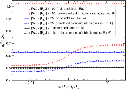
Figure 2: The noise of ${\mathrm{X}}$, $\sigma^{2}_{{\mathrm{X}}}/\langle{X}\rangle$ as a function of $d_{1}/k_{1}=d_{2}/k_{2}$ for a push-pull network for three different total substrate concentrations $[\mathrm{W_{\rm T}}]=[\mathrm{W}]+[\mathrm{E_{a}W}];[\mathrm{E_{a,T}}]=[\mathrm{E_{a}}]+[\mathrm{E_{a}W}]$ (see Eqs. 8). In all cases, the Michaelis-Menten constants were kept constant at $K_{M,E_{a}}=K_{M,E_{d}}=K_{M}=20$ $\mu$M. The horizontal solid lines correspond to the predictions of the noise addition rule (see Eq. 4), while the dotted curves correspond to the results of the full analysis that takes into account the correlations between the extrinsic and intrinsic noise. Note that as the substrate concentration increases, the push-pull network moves deeper into the zero-order regime and the noise in the output signal $\mathrm{X}$ increases. However, the actual increase is significantly lower than that predicted by the noise addition rule. The smaller increase in the output noise is due to the anti-correlations between the noise in the input signal and the intrinsic noise of the push-pull network. The decay rate of the enzyme $\mathrm{E_{a}}$ is $\lambda=30\,k_{1}$, while the production rate is chosen such that $[\mathrm{E_{a}}]=[\mathrm{E_{d}}]=0.2$ $\mu$M.

In the limit that both $d_{1}\gg k_{1}$ and $d_{2}\gg k_{2}$, the (un)binding reactions of the enzymes to the substrates can be integrated out and the reaction scheme reduces to

$${\mathrm{E_{a}}}+{\mathrm{W}}\,{\rightarrow}\,{\mathrm{E_{a}}}+{\mathrm{X}}$$ (9a)

$${\mathrm{E_{d}}}+{\mathrm{X}}\,{\rightarrow}\,{\mathrm{E_{d}}}+{\mathrm{W}}$$ (9b)

In this limit, the signal $\mathrm{E_{a}}$ is detected via scheme III (see Table 1); the modification and demodification rates are then given by Michaelis-Menten formulae Shibata and Fujimoto (2005). However, even in this limit, the spectral addition rule does not necessarily apply (see Fig. 2), as has been suggested Shibata and Fujimoto (2005). Because the total amount of $\mathrm{W}$ and $\mathrm{X}$ together is conserved, fluctuations in $\mathrm{X}$ are anti-correlated with those in $\mathrm{W}$ and hence with those in the fraction of enzyme $\mathrm{E_{a}}$ that is bound to its substrate $\mathrm{W}$. Since the bound enzyme is protected from deactivation, this effect will introduce anti-correlations between the fluctuations in the input signal $\mathrm{E_{a,T}}$ – the extrinsic noise – and those in the modification and demodification reactions – the intrinsic noise (see appendix C). This means that, even when $d_{1}\gg k_{1}$ and $d_{2}\gg k_{2}$, the spectral addition rule, and hence the noise addition rule, only holds when the fraction of bound enzyme is negligible (see Fig. 2).

It is commonly believed that one of the main biological functions of push-pull networks is to turn a graded input signal into a nearly binary output signal, thus allowing for an all-or-none response Goldbeter and Koshland, Jr. (1981); Ferrell, Jr. (1996). The amplification of input signals in push-pull networks strongly increases with increasing enzyme saturation Goldbeter and Koshland, Jr. (1981). Fig. 2 shows that as the substrate concentrations are increased (and the enzymes thus become more saturated with substrate), the noise in the output signal also markedly increases. This has been observed before Berg et al. (2000); Shibata and Fujimoto (2005): the higher gain not only amplifies the mean input signal, but also the noise in the input signal, the extrinsic noise Shibata and Fujimoto (2005); in addition, as the enzymes become more saturated with substrate, the intrinsic fluctuations of the network also increase, because the network moves deeper into the zero-order regime Berg et al. (2000). Our results show, however, that the actual increase in the output noise is much lower than that predicted by the noise addition rule. This is a result of the anti-correlations between the fluctuations in the input signal ($\mathrm{E_{a}}$) and the intrinsic noise of the network. These anti-correlations between the extrinsic and intrinsic noise reduce the noise in the output signal, but are neglected by the noise addition rule. Moreover, they become more important as the network moves deeper into the zero-order regime – as the enzymes $\mathrm{E_{a}}$ and $\mathrm{E_{d}}$ become more saturated with their substrates, the input signal $\mathrm{E_{a}}$ is increasingly being affected by its interaction with the detection component $\mathrm{W}$ of the network. While it is known that push-pull networks operating in the zero-order regime tend to exhibit large intrinsic fluctuations Berg et al. (2000); Rao et al. (2002), our results show that anti-correlations between the extrinsic and intrinsic noise temper these fluctuations.

	$\sigma^{2}_{\mathrm{Mos^{*}}}/{\left[\mathrm{Mos^{*}}\right]}$	$\sigma^{2}_{\mathrm{MEK-PP}}/{\left[{\mathrm{MEK-PP}}\right]}$	$\sigma^{2}_{\mathrm{MAPK-PP}}/{\left[{\mathrm{MAPK-PP}}\right]}$
Fully coupled ${\mathrm{Mos}}$, ${\mathrm{MEK}}$ and $\mathrm{MAPK}$	0.643	90.3	2.25
Spectral addition rule; all uncoupled	0.727	168.	3.75
Coupled ${\mathrm{Mos}}$ and ${\mathrm{MEK}}$; uncoupled $\mathrm{MAPK}$	0.643	91.1	2.26
Coupled ${\mathrm{MEK}}$ and ${\mathrm{MAPK}}$; uncoupled $\mathrm{Mos}$	0.727	166.	3.72

Table 3: Noise in the Mos/MEK/p42 MAPK cascade (see Fig. 1). “Full noise” refers to results of the analysis, in which the transmission of noise was computed by studying all the biochemical reactions together. “Spectral addition” corresponds to the results of the recursive application of the spectral addition rule to all the successive layers; the layers are thus assumed to form independent modules. “Coupled Mos and MEK; uncoupled MAPK” refers to the results of an analysis, in which the first two layers were considered to form one module, while the third layer was assumed to form an independent module; the transmission of noise from the first to the second layer was thus computed by taking into account the correlations between the fluctuations in the output signal of the first layer, the concentration of active Mos, and the intrinsic noise of the second layer, the intrinsic fluctuations of MEK; in contrast, the transmission of noise from the second to the third module was calculated using the spectral addition rule, thus ignoring these correlations. “Coupled MEK and MAPK; uncoupled Mos” corresponds to the analysis in which the first layer was considered to be independent, while the last two layers were considered to form one module. Note that the correlations between the noise in active Mos and the intrinsic fluctuations of MEK strongly affect the transmitted noise. The concentrations are: [Mos] = 3 nM; [MEK] = 1200 nM; [MAPK] = 300 nM. See appendix D for more details.

V Modularity and the MAPK cascade

We show the implications of the correlations between the extrinsic and intrinsic noise for a modular description of noise transmission in biochemical networks using a MAPK cascade that is based on the Mos/MEK/p42 MAPK cascade of Xenopus oocytes. From a topological point of view, this network consists of three push-pull modules that are connected in series. Their key features are shown in Fig. 1.

Active Mos can activate MEK through phosphorylation at two residues, while MEK, in turn, can activate p42 MAPK, also via double phosphorylation. The output signal of each of the modules, which provides the input signal for the next module in the cascade, is thus the active enzyme. We study here the network in which the feedback from p42 MAPK to Mos has been blocked Huang and Ferrell, Jr. (1996); Ferrell, Jr. and Machleder (1996). The rate constants and the protein concentrations were, as far as possible, taken from experiments Angeli et al. (2004); Ferrell, Jr. (1996); Huang and Ferrell, Jr. (1996) (see appendix D for details). All results have been obtained using the linear-noise approximations van Kampen (1992). These analytical results were found to be within 25% of numerical results of kinetic Monte Carlo simulations of the chemical master equation Bortz et al. (1975); Gillespie (1977). Appendix D describes in detail the linear-noise analysis.

Table 3 shows the noise in the output signals of the three modules, as predicted by an iterative application of the spectral addition rule to the successive modules and as revealed by the analysis that takes into account the correlations between the fluctuations in the input signal of a module (which is the output signal of its upstream module) and the intrinsic noise of that module (see appendix D). The spectral addition rule significantly overestimates the propagation of noise; the noise in MAPK, the output signal of the cascade, is about 50% lower than that predicted by the spectral addition rule. This supports our conclusion that anti-correlations between the extrinsic and intrinsic noise can enhance the performance of biochemical networks by making them more robust against biochemical noise.

Table 3 also illustrates under which conditions modularity can be exploited for a coarse-grained description of noise transmission. “Coupled Mos and MEK; uncoupled MAPK” refers to the results of an analysis, in which it is assumed that the first two layers together form one module, while the third layer constitutes a second, independent module. This analysis takes into account the correlations between the fluctuations in the output signal of the first layer – the concentration of active Mos – and the intrinsic fluctuations of the second layer – the noise in the modification and demodification reactions of MEK. However, it ignores the correlations between the output signal of the second layer and the intrinsic noise of the third layer. Similarly, “Coupled MEK and MAPK; uncoupled Mos” corresponds to the results of a description, in which the first layer forms one module, whereas the second and third layer form a second, independent module. We refer to appendix D for a mathematically precise description of the coupling between the respective layers.

It is seen that while the “Coupled Mos and MEK; uncoupled MAPK” description is fairly accurate, the “Coupled MEK and MAPK; uncoupled Mos” description significantly overestimates the noise in the output signal of the cascade. This shows that while the correlations between extrinsic and intrinsic noise are not very important for the transmission of noise from the second to the third layer, these correlations do strongly affect the propagation of noise from the first to the second layer. This difference is due to the differences in enzyme saturation: active Mos is more saturated with its substrate, MEK, than active MEK is with its substrate, MAPK. As a consequence, the signal that connects the first with the second layer (active Mos) is more affected by the detection reactions than that which connects the second with the third (active MEK).

VI Discussion

This analysis of the MAPK cascade unambiguously shows that correlations between the noise in the input signal of a network and the noise in the biochemical reactions that constitute the network, will affect the noise in the output signal of that network. It also shows the implications for a coarse-grained description of noise propagation in biochemical networks that, from a topological point of view, appear to consist of functionally independent modules Hartwell et al. (1999); Kashtan and Alon (2005); Angeli et al. (2004).

From the perspective of noise transmission, a network can be decomposed into modules only if the signals that connect them are detected via chemical reactions that do not introduce significant correlations between the noise in these signals and the intrinsic noise of the modules. Each module then has a characteristic noise input-output relation (Eq. 7) and this admits a modular description of noise transmission. The Mos-MEK/MAPK decomposition of the MAPK cascade illustrates this: the transmission of noise from the Mos-MEK subnetwork to the MAPK subnetwork can be described at the level of two independent modules connected in series, because the detection reactions do not affect the signal that connects the modules. If, however, the correlations between the extrinsic and intrinsic noise are significant, then the noise input-output relations of the different subnetworks become entangled and they no longer perform independently of one another, as the Mos/MEK-MAPK partitioning shows. In these cases, the propagation of noise can only be quantified accurately if the correlated subnetworks are regrouped into independent modules.

The effect of the correlations between the extrinsic and intrinsic noise is difficult to predict a priori. Our analytical expression for the power spectrum of the output signal (see Eq. 6) reveals that the effect on the noise in the output signal can either be positive or negative. This means that even if one would like to derive a lower or an upper bound on the transmitted noise, one has to explicitly take into account the correlations between the extrinsic and intrinsic noise. The noise addition rule, which neglects the correlations, makes uncontrolled assumptions and should thus be used with care Detwiler et al. (2000); Paulsson (2004); Shibata and Fujimoto (2005).

In general, the importance of the correlations between the extrinsic and intrinsic noise for the noise transmission is determined by the extent to which the signal is affected by the detection reactions. This increases when the concentration of the signaling molecules decreases with respect to that of the detection components (see Fig. 2). In zero-order ultrasensitive networks, the correlations are important, because the enzymes are saturated with substrate – the enzyme concentrations are thus low compared to the substrate concentrations. In gene regulatory networks, correlations between the fluctuations in the concentrations of the gene regulatory proteins, the extrinsic noise, and the intrinsic noise of gene expression, can contribute significantly to the transmission of noise through the network (to be published), because the concentrations of the gene regulatory proteins are often exceedingly low. The significance of the correlations between extrinsic and intrinsic noise also increases when the binding affinity of the signaling molecules for the detection component increases and/or when the detection reactions become slower (see Fig. 2). This is particularly important when weak signals have to be detected, as for example by the bacterium Escherichia coli, which can sense chemical attractants at nanomolar concentration Berg (2004). To be able to detect a weak signal, the processing network has to amplify the signal. This could be achieved by increasing the binding affinity of the signaling molecules. However, since the association rate cannot be increased beyond the diffusion-limited association rate constant, the only way to strongly increase the binding constant is to decrease the dissociation rate. As Fig. 2 shows, this will increase the importance of the correlations between the extrinsic and intrinsic noise. Correlations between extrinsic and intrinsic noise could thus impose strong design constraints for networks that have to detect small numbers of molecules. Lastly, we emphasize that any mechanism that increases the gain of a processing network, potentially also amplifies the effect of the correlations between the extrinsic and intrinsic noise. An interesting case is provided by the flagellar rotary motors of E. coli Berg (2004). Recent experiments have revealed that the probability of clockwise rotation depends very steeply on the concentration of the messenger protein; the effective Hill coefficient is about 10 Cluzel et al. (2000). This means that the noise in the rotation direction (the output signal of that system) is likely to be affected by the binding and unbinding of the messenger protein to the motor Bialek and Setayeshgar (2005) and thus to the correlations between the fluctuations in the messenger protein concentration (the extrinsic noise) and the intrinsic fluctuations of the motor switching (intrinsic noise).

Finally, we believe that the predictions of our analysis could be tested experimentally by performing fluorescence resonance energy transfer (FRET) or fluorescence correlation spectroscopy experiments on signal transduction pathways Sato et al. (2002); Sourjik and Berg (2002). The MAPK cascade would be an interesting model system. By putting a FRET donor on MEK, and a FRET acceptor on both the enzyme of the upstream module, Mos, and that of the downstream module, MAPK, it should be possible to study the effect of correlations between extrinsic and intrinsic noise on the transmission of noise in signal transduction cascades.

We thank Daan Frenkel, Bela Mulder, Rosalind Allen and Martin Howard for a critical reading of the manuscript. This work is supported by the Amsterdam Centre for Computational Science (ACCS). The work is part of the research program of the “Stichting voor Fundamenteel Onderzoek der Materie (FOM)", which is financially supported by the “Nederlandse organisatie voor Wetenschappelijk Onderzoek (NWO)".

Appendix A General analysis

We consider a general chemical network containing $N$ species $\{\mathrm{X}_{1},\mathrm{X}_{2},\dots,\mathrm{X}_{N}\}$. The state of the network is defined by the vector $\mathrm{\mathbf{X}}\equiv\{{X}_{1},{X}_{2},\dots,{X}_{N}\}$, where $X_{i}$ is the copy number of component $\rm{X_{i}}$. The $M$ reactions that constitute the network will be described by a propensity function ${\mathbf{A}}(\mathrm{\mathbf{X}})$ and a stoichiometric matrix $\mathrm{\mathbf{v}}^{i}$, where $\mathrm{v}^{i}_{j}$ denotes the change in the copy number of the species ${\mathrm{X}}_{j}$ due to reaction $i$. The reaction network dynamics can be modelled with a Chemical Master Equation, which describes the evolution of the probability $P(\mathbf{X},t)$ of having $X_{i}$ molecules of type $\mathrm{X}_{i}$

$$\frac{\text{d}P(\mathbf{X},t)}{\text{d}t}=\sum_{i=1}^{M}\left[A_{i}(\mathbf{X}-\mathbf{v}^{i})P(\mathbf{X}-\mathbf{v}^{i})-A_{i}(\mathbf{X})P(\mathbf{X})\right]$$ (10)

Following Gillespie (2000), the dynamics of the system can be approximated in the limit of large number of molecules by a Chemical Langevin Equation (CLE) of the form:

$$\frac{\text{d}\mathbf{X}}{\text{d}t}=\sum_{k=1}^{M}\mathbf{v}^{k}A_{k}(\mathbf{X})+\mathbf{\xi}$$ (11)

where $\mathbf{\xi}$ are Gaussian white noise terms of zero average and variance $\langle{\xi_{i}\xi_{j}}\rangle=\Xi_{ij}=\sum_{k=1}^{M}\mathbf{v}^{k}_{i}\mathbf{v}^{k}_{j}A_{k}(\mathbf{X})$. Setting the noise terms to zero one obtains the “deterministic rate equation”. The stable solutions of the equation

$$0=\sum_{k=1}^{M}\mathbf{v}^{k}A_{k}(\mathbf{X})$$ (12)

are usually a good approximation to the average values $\langle{\mathbf{X}}\rangle$ obtained from Eq. 10 in the limit of large volume van Kampen (1992). One can further simplify Eq. 11 by linearizing it around these solutions. One then obtains a set of linear stochastic differential equations for $\mathbf{x}=\mathbf{X}-\langle{\mathbf{X}}\rangle$. These represent the Linear Noise Approximation:

$$\frac{\text{d}x_{i}}{\text{d}t}=\sum_{j=1}^{N}F_{ij}x_{j}+\xi_{i}\quad\forall 0<i\leq N$$ (13)

where

$$F_{ij}=\sum_{k=1}^{M}\mathbf{v}^{k}_{i}\frac{\partial A_{k}(\langle{\mathbf{X}}\rangle)}{\partial X_{j}}$$ (14)

In this approximation, the noise characteristics (correlation matrix $\mathbf{\Xi}$) do not depend anymore on the dynamical variables (here, $\mathbf{x}$). The fluctuations of the variables $X_{i}$ are given by the correlation matrix $\mathbf{C}$, where $C_{ij}=\langle{x_{i}x_{j}}\rangle$. This correlation matrix can be obtained from the matrix equation Gardiner (2004)

$$\mathbf{FC}+\mathbf{CF}^{\dagger}=-\mathbf{\Xi}$$ (15)

The method that we have used to estimate the magnitude of the fluctuations of the components in the networks discussed below, consists of two steps: first, we set the noise terms to zero in the CLE to obtain the steady-state solutions of the resulting deterministic rate equation; second, we compute the force matrix $\mathbf{F}$ and the noise correlations $\mathbf{\Xi}$ in these points in order to obtain the correlation matrix $\mathbf{C}$. In what follows, we will refer to the value of the matrix element $C_{ii}$ as the noise in component $\rm{X_{i}}$. We have verified the accuracy of the Linear Noise Approximation for the problems discussed here by comparing the results with those of kinetic Monte Carlo simulations of the chemical master equation (Eq. 10) Bortz et al. (1975); Gillespie (1977).

Appendix B General Processing Network and Modularity

Let us consider a linear(ized) reaction network of $N$ components using the following set of Chemical Langevin Equations:

$$\dot{x}_{i}=\sum_{j=1}^{M}G_{ij}s_{j}+\sum_{j=1}^{N}A_{ij}x_{j}+\xi_{i}\quad\forall\,i=1\dots N.$$ (16)

Here, $x_{j}$ are the components of the processing network and $s_{j}$ denote the input signals. $A_{ij}$ are coefficients, $G_{ij}$ are transmission factors, and $\mathbf{\xi}$ model the noise in the network components; we model them as Gaussian white noise of zero average and with $\langle{\xi_{i}(t)\xi_{j}(t^{\prime})}\rangle=\Xi_{ij}\delta(t-t^{\prime})$. Crucially, in general, $\mathbf{s}$ depends upon the history of the values of the network components. Using the linearity of Eq. 16, the Fourier transform of the outputs ${\mathrm{X}}_{i}$ can be found from an algebraic equation with solution

$$\tilde{x}_{i}(\omega)=-\sum_{j=1}^{N}B_{ij}\left[\sum_{k=1}^{M}(G_{jk}\tilde{s}_{k}(\omega))+\tilde{\xi}_{j}(\omega)\right],$$ (17)

where the matrix $\mathbf{B}$ is given by $\mathbf{B}=\left(\mathbf{A}+\text{i}\omega\right)^{-1}$. The corresponding power spectrum is:

$$S_{\mathrm{X}_{i}}(\omega)=\sum_{k,j=1}^{N}B^{\dagger}_{ki}(\omega)B_{ij}(\omega)\Xi_{jk}+\sum_{j,l=1}^{N}\sum_{k,m=1}^{M}B_{ij}(\omega)G_{jk}\langle{\tilde{s}_{k}(\omega)\tilde{s}^{*}_{m}(\omega)}\rangle G^{\dagger}_{ml}B^{\dagger}_{li}(\omega)+$$

$$+\sum_{j,l=1}^{N}\sum_{k=1}^{M}B_{ij}(\omega)\left[G_{jk}C_{\mathrm{S}_{k}\xi_{l}}(\omega)+G_{lk}C^{*}_{\mathrm{S}_{k}\xi_{j}}(\omega)\right]B^{\dagger}_{li}(\omega).$$ (18)

Here, $\tilde{C}_{\mathrm{S}\xi}(\omega)$ denotes the correlation between the input signal and the noise $\xi$ in the frequency domain. The first term of the rhs of Eq. 18 is the power spectrum of the intrinsic noise of ${\mathrm{X}}_{i}$, while the second term is the spectrum of the signal $s_{j}$ modulated by an intrinsic transfer function. If the input signals are uncorrelated with each other ($\langle{\tilde{s}_{k}(\omega)\tilde{s}^{*}_{m}(\omega)}\rangle=\delta_{km}S_{\mathrm{S}_{k}}(\omega)$) and uncorrelated with the detection network ($\tilde{C}_{\mathrm{S}\xi}(\omega)=0$), Eq. 18 reduces to

$$S_{\mathrm{X}_{i}}(\omega)=S_{\mathrm{X}_{i}}^{\mathrm{in}}(\omega)+\sum_{j=1}^{M}g_{\mathrm{X}_{i}}^{\mathrm{S}_{j}}S_{\mathrm{S}_{k}}(\omega),$$ (19)

where $S_{\mathrm{X}_{i}}^{\mathrm{in}}(\omega)=\sum_{k,j=1}^{N}B^{\dagger}_{ki}(\omega)B_{ij}(\omega)\Xi_{jk}$ is the intrinsic noise and $g_{\mathrm{X}_{i}}^{\mathrm{S}_{k}}=\sum_{j,l=1}^{N}B_{ij}(\omega)G_{jk}G^{\dagger}_{kl}B^{\dagger}_{li}(\omega)$ are intrinsic transfer functions, both independent of the input signals. This is the spectral addition rule (Eq.7 of the manuscript) for a general linear(ized) reaction network that detects multiple input signals via detection scheme III. Importantly, in this case the power spectra of the input signals $S_{{\rm S}_{i}}(\omega)=\langle\tilde{s}_{i}(\omega)\tilde{s}^{*}_{i}(\omega)\rangle$ are unaffected by their interactions with the processing network; conversely, the intrinsic contribution to the power spectrum of ${\rm X}_{i}$, $S_{\mathrm{X}_{i}}^{\mathrm{in}}(\omega)$, is a truly intrinsic quantity that depends upon properties of the processing module only, and not upon the fluctuations in the input signals, given by $S_{\mathrm{S}_{k}}(\omega)$. However, if the input signals are correlated with each other and/or detected via scheme I and/or II, then the power spectra of the input signals and those of the network do mutually affect each other and the spectral addition rule breaks down. We emphasize that even when the input signals do not directly interact with the components that provide the output signals (as in the section II), but only indirectly via chemical reactions of the type of scheme I and II, then cross-correlations in the noise $\langle{\xi_{i}\xi_{j}}\rangle$ can be important, because their effects can propagate from the input signals to the output signals. From the perspective of noise transmission, a network can be decomposed into modules by cutting the network links that correspond to chemical reactions of the type in scheme III.

Appendix C Zero-Order Ultrasensitive push-pull module

Let us consider the network:

	$\mathrm{W}+\mathrm{E_{a}}\underset{d_{1}}{\overset{a_{1}}{\rightleftarrows}}\mathrm{E_{a}W}\overset{k_{1}}{\longrightarrow}\mathrm{E_{a}+X}$
	$\mathrm{X}+\mathrm{E_{d}}\underset{d_{2}}{\overset{a_{2}}{\rightleftarrows}}\mathrm{E_{d}X}\overset{k_{2}}{\longrightarrow}\mathrm{E_{d}+W}$

The input signal is provided by the enzyme $\mathrm{E_{a}}$. Its activation and deactivation dynamics is modeled as a birth-death process:

$$\emptyset\overset{k}{\longrightarrow}\mathrm{E_{a}}\overset{\lambda}{\longrightarrow}\emptyset$$ (20)

Michaelis-Menten formulae can be derived by assuming fast equilibration of the complexes $\mathrm{E_{a}W}$ and $\mathrm{E_{d}X}$. In order to self-consistently eliminate these intermediates, we split the independent variables into slow variables – those that do not change in the fast (un)binding reactions – and fast variables. We thus define the following slow variables: $\mathrm{W_{T}}=\mathrm{W}+\mathrm{E_{a}W}$, $\mathrm{X_{T}}=\mathrm{X}+\mathrm{E_{d}X}$, $\mathrm{E_{a,T}}=\mathrm{E_{a}}+\mathrm{E_{a}W}$ and $\mathrm{E_{d,T}}=\mathrm{E_{d}}+\mathrm{E_{d}X}$. The independent variables therefore are:

$$\mathrm{\mathbf{X}}=\{\mathrm{\mathbf{X}}_{s},\mathrm{\mathbf{X}}_{f}\},\quad\mathrm{\mathbf{X}}_{s}=\{E_{a,T},X_{T}\},\quad\mathrm{\mathbf{X}}_{f}=\{E_{a}W,E_{d}X\}.$$ (21)

We also use the conservation laws $W+E_{a}W+X+E_{d}X=Y=\mbox{constant}$ and $E_{d}+E_{d}X=E_{d,T}$. The values of the constants $Y$ and $E_{d,T}$ will appear as parameters in the dynamics of the network. For the full network, in the new variables, we have

$$\mathbf{F}=\begin{bmatrix}-\lambda&0&\lambda&0\\ 0&0&k_{1}&-k_{2}\\ a_{1}\langle{W}\rangle&-a_{1}\langle{E_{a}}\rangle&-d_{1}-k_{1}-a_{1}\langle{W+E_{a}}\rangle&0\\ 0&a_{2}E_{d}&0&-d_{2}-k_{2}-a_{2}\langle{X-E_{d}}\rangle\end{bmatrix}\mbox{, and}$$ (22)

$$\mathbf{\Xi}=\begin{bmatrix}k+\lambda\langle{E_{a}}\rangle&0&0&0\\ 0&k_{1}\langle{E_{a}}\rangle+k_{2}\langle{E_{d}X}\rangle&-k_{1}\langle{E_{a}W}\rangle&k_{2}\langle{E_{d}X}\rangle\\ 0&-k_{1}\langle{E_{a}W}\rangle&(d_{1}+k_{1})\langle{E_{a}W}\rangle+a_{1}\langle{E_{a}}\rangle\langle{W}\rangle&0\\ 0&k_{2}\langle{E_{d}X}\rangle&0&(d_{2}+k_{2})\langle{E_{d}X}\rangle+a_{2}\langle{E_{d}}\rangle\langle{X}\rangle\end{bmatrix}$$ (23)

In the limit of large (un)binding rates ($a,d\gg k$), the copy numbers of the enzyme-substrate complexes can be expressed as a function of those of the slow variables

$$E_{a}W(X_{T},E_{a,T}) = \frac{{E_{a,T}}+{K_{\mathrm{m}1}}+(Y-X_{T})-{\sqrt{{{\left({E_{a,T}}+{K_{\mathrm{m}1}}+Y-X_{T}\right)}^{2}}-4\,{E_{a,T}}\left(Y-X_{T}\right)}}}{2}$$

$$E_{d}X(X_{T},E_{a,T}) = \frac{{E_{d,T}}+{K_{\mathrm{m}2}}+X_{T}-{\sqrt{{{\left({E_{d,T}}+{K_{\mathrm{m}2}}+X_{T}\right)}^{2}}-4\,{E_{d,T}}\,X_{T}}}}{2}.$$ (24)

It is seen that the concentrations of the complexes depend on the rates $a_{i}$, $d_{i}$ and $k_{i}$ only through the Michaelis-Menten constants $K_{\mathrm{m}i}=(d_{i}+k_{i})/a_{i}$. The network dynamics can be reduced to the simple form of a two-dimensional Chemical Langevin Equation, depending only on $K_{\mathrm{m}i}$ and $k_{i}$:

$$\frac{\text{d}X_{T}}{\text{d}t} =k_{1}\,E_{a}W(X_{T},E_{a,T})-k_{2}\,E_{d}X(X_{T},E_{a,T})+\xi_{\mathrm{X_{T}}}$$ (25a)

$$\frac{\text{d}E_{a,T}}{\text{d}t} =k-\lambda\,\left[E_{a,T}-E_{a}W(X_{T},E_{a,T})\right]+\xi_{\mathrm{E_{a,T}}}$$ (25b)

In order to compute the noise in the network components within the Linear Noise Approximation we use the matrices

$$\mathbf{F}=\begin{bmatrix}-\lambda+\lambda\frac{\partial E_{a}W(X_{T},E_{a,T})}{\partial E_{a,T}}&\lambda\frac{\partial E_{a}W(X_{T},E_{a,T})}{\partial X_{T}}\\ k_{1}\frac{\partial E_{a}W(X_{T},E_{a,T})}{\partial E_{a,T}}-k_{2}\frac{\partial E_{d}X(X_{T},E_{a,T})}{\partial E_{a,T}}&k_{1}\frac{\partial E_{a}W(X_{T},E_{a,T})}{\partial X_{T}}-k_{2}\frac{\partial E_{d}X(X_{T},E_{a,T})}{\partial X_{T}}\\ \end{bmatrix}$$ (26)

and

$$\mathbf{\Xi}=\begin{bmatrix}k+\lambda\langle{E_{a}}\rangle&0\\ 0&k_{1}\langle{E_{a}}\rangle+k_{2}\langle{E_{d}X}\rangle\\ \end{bmatrix}.$$ (27)

The prediction of the noise addition rule for the noise in $\mathrm{X_{T}}$ is obtained by setting the feedback $F_{1,2}$ to zero, such that

$$\mathbf{F_{NA}}=\begin{bmatrix}-\lambda+\lambda\frac{\partial E_{a}W(X_{T},E_{a,T})}{\partial E_{a,T}}&0\\ k_{1}\frac{\partial E_{a}W(X_{T},E_{a,T})}{\partial E_{a,T}}-k_{2}\frac{\partial E_{d}X(X_{T},E_{a,T})}{\partial E_{a,T}}&k_{1}\frac{\partial E_{a}W(X_{T},E_{a,T})}{\partial X_{T}}-k_{2}\frac{\partial E_{d}X(X_{T},E_{a,T})}{\partial X_{T}}\\ \end{bmatrix}.$$ (28)

It is perhaps instructive to compare the approach presented here to that commonly employed for enzymatic reactions Detwiler et al. (2000); Berg et al. (2000); Shibata and Fujimoto (2005), which would write the reactions for the push-pull network as:

$$\mathrm{W}\underset{k_{d}}{\overset{k_{a}}{\rightleftarrows}}\mathrm{X};\,\,k_{a}=\frac{k_{1}E_{a,T}\,W}{W+K_{\mathrm{m}1}};\,\,k_{d}=\frac{k_{2}E_{d,T}\,X}{X+K_{\mathrm{m}2}}$$ (29)

A connection can be made by noting that, when the binding and unbinding of the enzymes to the substrates is fast, $E_{a}W=E_{a,T}W/(K_{{\rm m},1}+W)$ and $E_{d}X=E_{d,T}X/(K_{{\rm m},2}+X)$; it can be verified that these expressions are equivalent to those for $E_{a}W$ and $E_{d}X$ in Eq. C. However, the principal difference between our approach and that presented in Detwiler et al. (2000); Berg et al. (2000); Shibata and Fujimoto (2005) is that we analyze the dynamics of $E_{aT}$ and $X_{T}$ together, thus taking into the fact that the fluctuations in $X_{T}$ can act back on those in $E_{aT}$. If the fraction of enzyme $\rm{E_{a}}$ that is bound to its substrate, $\rm{W}$, is small, then the importance of the third term in Eq. 25b (involving the complex $E_{a}W$) is small. In this limit, the results of the full analysis, which takes into account the correlations between the extrinsic and intrinsic noise, reduces to those of the spectral addition rule (see Fig. 2).

$\mathrm{Mos}+\mathrm{E_{1}}\underset{d_{1}}{\overset{a_{1}}{\rightleftarrows}}\mathrm{E_{1}Mos}\overset{k_{1}}{\longrightarrow}\mathrm{E_{1}+Mos^{*}}$
$\mathrm{Mos^{*}}+\mathrm{E_{2}}\underset{d_{2}}{\overset{a_{2}}{\rightleftarrows}}\mathrm{E_{2}Mos^{*}}\overset{k_{2}}{\longrightarrow}\mathrm{E_{2}+Mos}$
$\mathrm{MEK}+\mathrm{Mos^{*}}\underset{d_{3}}{\overset{a_{3}}{\rightleftarrows}}\mathrm{Mos^{*}MEK}\overset{k_{3}}{\longrightarrow}\mathrm{Mos^{*}+MEK\!\!\!-\!\!\!P}$
$\mathrm{MEK\!\!\!-\!\!\!P}+\mathrm{MEKP^{\prime}ase}\underset{d_{4}}{\overset{a_{4}}{\rightleftarrows}}\mathrm{MEKP^{\prime}aseMEK\!\!\!-\!\!\!P}\overset{k_{4}}{\longrightarrow}\mathrm{MEKP^{\prime}ase+MEK}$
$\mathrm{MEK\!\!\!-\!\!\!P}+\mathrm{Mos^{*}}\underset{d_{5}}{\overset{a_{5}}{\rightleftarrows}}\mathrm{Mos^{*}MEK\!\!\!-\!\!\!P}\overset{k_{5}}{\longrightarrow}\mathrm{Mos^{*}+MEK\!\!\!-\!\!\!PP}$
$\mathrm{MEK\!\!\!-\!\!\!PP}+\mathrm{MEKP^{\prime}ase}\underset{d_{6}}{\overset{a_{6}}{\rightleftarrows}}\mathrm{MEKP^{\prime}aseMEK\!\!\!-\!\!\!PP}\overset{k_{5}}{\longrightarrow}\mathrm{MEKP^{\prime}ase+MEK\!\!\!-\!\!\!P}$
$\mathrm{MAPK}+\mathrm{MEK\!\!\!-\!\!\!PP}\underset{d_{7}}{\overset{a_{7}}{\rightleftarrows}}\mathrm{MEK\!\!\!-\!\!\!PPMAPK}\overset{k_{7}}{\longrightarrow}\mathrm{MEK\!\!\!-\!\!\!PP+MAPPK\!\!\!-\!\!\!P}$
$\mathrm{MAPK\!\!\!-\!\!\!P}+\mathrm{MAPKP^{\prime}ase}\underset{d_{8}}{\overset{a_{8}}{\rightleftarrows}}\mathrm{MAPKP^{\prime}aseMAPK\!\!\!-\!\!\!P}\overset{k_{8}}{\longrightarrow}\mathrm{MAPKP^{\prime}ase+MAPK}$
$\mathrm{MAPK\!\!\!-\!\!\!P}+\mathrm{MEK\!\!\!-\!\!\!PP}\underset{d_{9}}{\overset{a_{9}}{\rightleftarrows}}\mathrm{MEK\!\!\!-\!\!\!PPMAPK\!\!\!-\!\!\!P}\overset{k_{9}}{\longrightarrow}\mathrm{MEK\!\!\!-\!\!\!PP+MAPPK\!\!\!-\!\!\!PP}$
$\mathrm{MAPK\!\!\!-\!\!\!PP}+\mathrm{MAPKP^{\prime}ase}\underset{d_{10}}{\overset{a_{10}}{\rightleftarrows}}\mathrm{MAPKP^{\prime}aseMAPK\!\!\!-\!\!\!PP}\overset{k_{10}}{\longrightarrow}\mathrm{MAPKP^{\prime}ase+MAPK\!\!\!-\!\!\!P}$

Table 4: Reactions in the MAPK cascade.

Appendix D MAPK cascade

We model the Mos/MEK/p42 MAPK cascade as a network consisting of 10 enzymatic reactions Huang and Ferrell, Jr. (1996); these are listed in Table 4.

Since the association and deassociation rates ($a_{i}$ and $d_{i}$, respectively) have not been measured experimentally, we consider the limit of fast binding and unbinding. We are thus interested in the dynamics of the slow components:

$$\mathrm{Mos^{*}_{T}} \equiv \mathrm{Mos^{*}}+\mathrm{E_{2}Mos^{*}}+\mathrm{Mos^{*}MEK}+\mathrm{Mos^{*}MEK\!\!\!-\!\!\!P}$$

$$\mathrm{MEK\!\!\!-\!\!\!P_{T}} \equiv \mathrm{MEK\!\!\!-\!\!\!P}+\mathrm{Mos^{*}MEK\!\!\!-\!\!\!P}+\mathrm{MEKP^{\prime}aseMEK\!\!\!-\!\!\!P}$$

$$\mathrm{MEK\!\!\!-\!\!\!PP_{T}} \equiv \mathrm{MEK\!\!\!-\!\!\!PP}+\mathrm{MEKP^{\prime}aseMEK\!\!\!-\!\!\!PP}+\mathrm{MEK\!\!\!-\!\!\!PPMAPK}+\mathrm{MEK\!\!\!-\!\!\!PPMAPK\!\!\!-\!\!\!P}$$

$$\mathrm{MAPK\!\!\!-\!\!\!P_{T}} \equiv \mathrm{MAPK\!\!\!-\!\!\!P}+\mathrm{MEK\!\!\!-\!\!\!PPMAPK\!\!\!-\!\!\!P}+\mathrm{MAPKP^{\prime}aseMAPK\!\!\!-\!\!\!P}$$

$$\mathrm{MAPK\!\!\!-\!\!\!PP_{T}} \equiv \mathrm{MAPK\!\!\!-\!\!\!PP}+\mathrm{MAPKP^{\prime}aseMAPK\!\!\!-\!\!\!PP}$$ (30)

We use the conservation laws:

$$\mathrm{E_{1,T}} = \mathrm{E_{1}}+\mathrm{E_{1}Mos}=\mathrm{constant}$$

$$\mathrm{Mos_{T}} = \mathrm{Mos^{*}_{T}}+\mathrm{Mos}+\mathrm{E_{1}Mos}=\mathrm{constant}$$

$$\mathrm{E_{2,T}} = \mathrm{E_{2}}+\mathrm{E_{2}Mos^{*}}=\mathrm{constant}$$

$$\mathrm{MEK_{T}} = \mathrm{MEK\!\!\!-\!\!\!P_{T}}+\mathrm{MEK\!\!\!-\!\!\!PP_{T}}+\mathrm{MEK}+\mathrm{Mos^{*}MEK}=\mathrm{constant}$$

$$\mathrm{MEKP^{\prime}ase_{T}} = \mathrm{MEKP^{\prime}ase}+\mathrm{MEKP^{\prime}aseMEK\!\!\!-\!\!\!P}+\mathrm{MEKP^{\prime}aseMEK\!\!\!-\!\!\!PP}=\mathrm{constant}$$

$$\mathrm{MAPK_{T}} = \mathrm{MAPK}+\mathrm{MAPK\!\!\!-\!\!\!P_{T}}+\mathrm{MAPK\!\!\!-\!\!\!PP_{T}}+\mathrm{MEK\!\!\!-\!\!\!PPMAPK}=\mathrm{constant}$$ (31)

$$\mathrm{MAPKP^{\prime}ase_{T}} = \mathrm{MAPKP^{\prime}ase}+\mathrm{MAPKP^{\prime}aseMAPK\!\!\!-\!\!\!P}+\mathrm{MAPKP^{\prime}aseMAPK\!\!\!-\!\!\!PP}=\mathrm{constant}$$

For the slow variables, the Chemical Langevin Equations read:

$$\frac{\text{d}}{\text{d}t}Mos^{*}_{T} = k_{1}E_{1}Mos-k_{2}E_{2}Mos^{*}+\xi_{1}$$

$$\frac{\text{d}}{\text{d}t}MEK\!\!\!-\!\!\!P_{T} = k_{3}Mos^{*}MEK-k_{4}MEKP^{\prime}aseMEK\!\!\!-\!\!\!P-$$

$$k_{5}Mos^{*}MEK\!\!\!-\!\!\!P+k_{6}MEKP^{\prime}aseMEK\!\!\!-\!\!\!PP+\xi_{2}$$

$$\frac{\text{d}}{\text{d}t}MEK\!\!\!-\!\!\!PP_{T} = k_{5}Mos^{*}MEK\!\!\!-\!\!\!P-k_{6}MEKP^{\prime}aseMEK\!\!\!-\!\!\!PP+\xi_{3}$$

$$\frac{\text{d}}{\text{d}t}MAPK\!\!\!-\!\!\!P_{T} = k_{7}{MEK\!\!\!-\!\!\!PPMAPK}-k_{8}{MAPKP^{\prime}aseMAPK\!\!\!-\!\!\!P}-$$

$$k_{9}MEK\!\!\!-\!\!\!PPMAPK\!\!\!-\!\!\!P+k_{10}MAPKP^{\prime}aseMAPK\!\!\!-\!\!\!PP+\xi_{4}$$

$$\frac{\text{d}}{\text{d}t}{MAPK\!\!\!-\!\!\!PP_{T}} = k_{9}MEK\!\!\!-\!\!\!PPMAPK\!\!\!-\!\!\!P-k_{10}MAPKP^{\prime}aseMAPK\!\!\!-\!\!\!PP+\xi_{5}$$ (32)

where the noise terms $\mathbf{\xi}$, as discussed above, are modeled as Gaussian white noise of zero mean and variance:

$$\langle{\xi_{1}^{2}}\rangle = k_{1}E_{1}Mos+k_{2}E_{2}Mos^{*}$$

$$\langle{\xi_{2}^{2}}\rangle = k_{3}Mos^{*}MEK+k_{4}MEKP^{\prime}aseMEK\!\!\!-\!\!\!P+$$

$$k_{5}Mos^{*}MEK\!\!\!-\!\!\!P+k_{6}MEKP^{\prime}aseMEK\!\!\!-\!\!\!PP$$

$$\langle{\xi_{3}^{2}}\rangle = k_{5}Mos^{*}MEK\!\!\!-\!\!\!P+k_{6}MEKP^{\prime}aseMEK\!\!\!-\!\!\!PP$$

$$\langle{\xi_{4}^{2}}\rangle = k_{7}{MEK\!\!\!-\!\!\!PPMAPK}+k_{8}{MAPKP^{\prime}aseMAPK\!\!\!-\!\!\!P}+$$

$$k_{9}MEK\!\!\!-\!\!\!PPMAPK\!\!\!-\!\!\!P+k_{10}MAPKP^{\prime}aseMAPK\!\!\!-\!\!\!PP$$

$$\langle{\xi_{5}^{2}}\rangle = k_{9}MEK\!\!\!-\!\!\!PPMAPK\!\!\!-\!\!\!P+k_{10}MAPKP^{\prime}aseMAPK\!\!\!-\!\!\!PP$$ (33)

All the noise terms are uncorrelated, except:

$$\langle{\xi_{2}\xi_{3}}\rangle=-\left(k_{5}Mos^{*}MEK\!\!\!-\!\!\!P+k_{6}MEKP^{\prime}aseMEK\!\!\!-\!\!\!PP\right)$$

$$\langle{\xi_{4}\xi_{5}}\rangle=-\left(k_{9}MEK\!\!\!-\!\!\!PPMAPK\!\!\!-\!\!\!P+k_{10}MAPKP^{\prime}aseMAP\right)$$ (34)

The noise correlations $\langle{\xi_{i}\xi_{j}}\rangle$ define the elements of the matrix $\mathbf{\Xi}$.

The dependence of the intermediate complexes $\mathrm{E_{1}Mos}$, $\mathrm{E_{2}Mos^{*}}$, $\mathrm{Mos^{*}MEK}$, $\mathrm{Mos^{*}MEK\!\!\!-\!\!\!P}$, $\mathrm{MEKP^{\prime}aseMEK\!\!\!-\!\!\!P}$, $\mathrm{MEKP^{\prime}aseMEK\!\!\!-\!\!\!PP}$, $\mathrm{MEK\!\!\!-\!\!\!PPMAPK}$, $\mathrm{MEK\!\!\!-\!\!\!PPMAPK\!\!\!-\!\!\!P}$, $\mathrm{MAPKP^{\prime}aseMAPK\!\!\!-\!\!\!P}$, and $\mathrm{MAPKP^{\prime}aseMAPK\!\!\!-\!\!\!PP}$ on the slow variables around the steady state, has been obtained numerically. The concentrations of the complexes depend on the reaction rates only through the Michaelis-Menten constants $K_{\mathrm{m}i}=(d_{i}+k_{i})/a_{i}$.

We can now construct, as explained in section A, the force matrix $\mathbf{F}$ of the Linear Noise approximation and use $\mathbf{F}$ and $\mathbf{\Xi}$ as defined in Eqs. D and D to numerically solve Eq. 15.

The MAPK network consists of three layers. Here we address the question to what extent these can be described as three independent modules. To this end, we divide the full network into subnetworks, in three different manners:

$$\mathrm{1.} \{\mathrm{Mos^{*}_{T}}\} \{\mathrm{MEK\!\!\!-\!\!\!P_{T}},\mathrm{MEK\!\!\!-\!\!\!PP_{T}}\}\quad\{\mathrm{MAPK\!\!\!-\!\!\!P_{T}},\mathrm{MAPK\!\!\!-\!\!\!PP_{T}}\}$$

$$\mathrm{2.} \{\mathrm{Mos^{*}_{T}},\mathrm{MEK\!\!\!-\!\!\!P_{T}},\mathrm{MEK\!\!\!-\!\!\!PP_{T}}\} \{\mathrm{MAPK\!\!\!-\!\!\!P_{T}},\mathrm{MAPK\!\!\!-\!\!\!PP_{T}}\}$$

$$\mathrm{3.} \{\mathrm{Mos^{*}_{T}}\} \{\mathrm{MEK\!\!\!-\!\!\!P_{T}},\mathrm{MEK\!\!\!-\!\!\!PP_{T}},\mathrm{MAPK\!\!\!-\!\!\!P_{T}},\mathrm{MAPK\!\!\!-\!\!\!PP_{T}}\}$$ (35)

The network numbered 1 consists of three uncoupled layers; that numbered 2 consists of one module in which the Mos and the MEK layer are coupled, while the MAPK layer is assumed to form a second, independent module; network 3 consists of one module in which layers 2 and 3 are concatenated and one, uncoupled, module formed by layer 1.

To study the effect of the correlations between the extrinsic and intrinsic noise, it is instructive to define submatrices, $\bf{F_{ii}}$, $\bf{G_{ij}}$ ($i>j$), and $\bf{K_{ij}}$ ($i<j$) of the matrix $\bf{F}$ of the full network. These matrices are defined as follows:

$$\begin{bmatrix}\mathbf{F_{11}}&\mathbf{K_{12}}&\mathbf{K_{13}}\\ \mathbf{G_{21}}&\mathbf{F_{22}}&\mathbf{K_{23}}\\ \mathbf{G_{31}}&\mathbf{G_{32}}&\mathbf{F_{33}}\\ \end{bmatrix}\equiv\mathbf{F}.$$ (36)

The three decompositions of the full network then correspond to the following force matrices:

$$\mbox{1}: \hskip 14.22636pt\mathbf{F_{1}}\equiv\begin{bmatrix}\mathbf{F_{11}}&\mathbf{0}&\mathbf{0}\\ \mathbf{G_{21}}&\mathbf{F_{22}}&\mathbf{0}\\ \mathbf{0}&\mathbf{G_{32}}&\mathbf{F_{33}}\;\\ \end{bmatrix}$$ Spectral Addition; All Uncoupled

$$\mbox{2}: \hskip 14.22636pt\mathbf{F_{2}}\equiv\begin{bmatrix}\mathbf{F_{11}}&\mathbf{K_{12}}&\mathbf{0}\\ \mathbf{G_{21}}&\mathbf{F_{22}}&\mathbf{0}\\ \mathbf{0}&\mathbf{G_{32}}&\mathbf{F_{33}}\;\\ \end{bmatrix}$$ Coupled Mos and MEK; Uncoupled MAPK

$$\mbox{3}: \hskip 14.22636pt\mathbf{F_{3}}\equiv\begin{bmatrix}\mathbf{F_{11}}&\mathbf{0}&\mathbf{0}\\ \mathbf{G_{21}}&\mathbf{F_{22}}&\mathbf{K_{23}}\\ \mathbf{0}&\mathbf{G_{32}}&\mathbf{F_{33}}\\ \end{bmatrix}$$ Uncoupled Mos; Coupled MEK and MAPK

Here, $\mathbf{0}$ is the null matrix.

$\mathrm{Mos_{T}}$	$\mathrm{MEK_{T}}$	$\mathrm{MAPK_{T}}$	$\quad\mathrm{E_{1,T}}\quad$	$\quad\mathrm{E_{2,T}}\quad$	$\mathrm{MEKP^{\prime}ase_{T}}$	$\mathrm{MAPKP^{\prime}ase_{T}}$
3	1200	300	0.1	0.6	0.6	300

Table 5: Total concentrations of the components (nM)

The noise matrix $\mathbf{\Xi}$ of the full network is already partitioned into the different modules. For all partitionings, the noise matrix is thus given by Eqs. D and D.

The relevant model parameters are the total concentrations on the rhs of Eq. D and the Michaelis-Menten constants. The concentrations were taken from the experiments discussed in Ferrell, Jr. (1996); Huang and Ferrell, Jr. (1996); Angeli et al. (2004); Mansour et al. (1996) and are shown in Table 5. The Michaelis-Menten constant of the MAPK activation by MEK has been measured experimentally Mansour et al. (1996). Following Huang and Ferrell, Jr. (1996); Angeli et al. (2004), we take all Michaelis-Menten constants to be equal to $K_{\rm mi}=K_{\rm M}=300\,$ nM. The $k_{i}$ values were taken to be equal to each other; their absolute value is not important for the calculations here, because it only sets the time scale in the problem.

References

- McAdams and Arkin (1997) H. H. McAdams and A. Arkin, Proc. Natl. Acad. Sci. USA 94, 814 (1997).
- Elowitz and Leibler (2000) M. B. Elowitz and S. Leibler, Nature 403, 335 (2000).
- Ozbudak et al. (2002) E. M. Ozbudak, M. Thattai, I. Kurtser, A. D. Grossman, and A. van Oudenaarden, Nat. Gen. 31, 69 (2002).
- Elowitz et al. (2002) M. B. Elowitz, A. J. Levine, E. D. Siggia, and P. S. Swain, Science 297, 1183 (2002).
- Ozbudak et al. (2004) E. M. Ozbudak, M. Thattai, H. N. Lim, B. I. Shraiman, and A. van Oudenaarden, Nature 427, 737 (2004).
- Pedraza and van Oudenaarden (2005) J. M. Pedraza and A. van Oudenaarden, Science 307, 1965 (2005).
- Rosenfeld et al. (2005) N. Rosenfeld, J. W. Young, U. Alon, P. S. Swain, and M. B. Elowitz, Science 307, 1962 (2005).
- Blake et al. (2003) W. J. Blake, M. Kaern, C. R. Cantor, and J. J. Collins, Nature 422, 633 (2003).
- Raser and O’Shea (2004) J. M. Raser and E. K. O’Shea, Science 304, 1811 (2004).
- Acar et al. (2005) M. Acar, A. Becksei, and A. van Oudenaarden, Nature 435, 228 (2005).
- Becksei et al. (2005) A. Becksei, B. B. Kaufmann, and A. van Oudenaarden, Nat. Genet. 37, 937 (2005).
- Colman-Lerner et al. (2005) A. Colman-Lerner, A. Gordon, E. Serra, T. Chin, O. Resnekov, D. Endy, G. Pesce, and R. Brent, Nature 437, 699 (2005).
- Korobkova et al. (2004) E. Korobkova, T. Emonet, J. M. G. Vilar, T. S. Shimizu, and P. Cluzel, Nature 428, 574 (2004).
- Rao et al. (2002) C. V. Rao, D. M. Wolf, and A. P. Arkin, Nature 420, 231 (2002).
- Kaern et al. (2005) M. Kaern, T. C. Elston, W. J. Blake, and J. J. Collins, Nat. Rev. Genet. 6, 451 (2005).
- Paulsson et al. (2000) J. Paulsson, O. G. Berg, and M. Ehrenberg, Proc. Natl. Acad. Sci. USA 97, 7148 (2000).
- Vilar et al. (2002) J. M. G. Vilar, H. Y. Kueh, N. Barkai, and S. Leibler, Proc. Natl. Acad. Sci. USA 99, 5988 (2002).
- Thattai and van Oudenaarden (2004) M. Thattai and A. van Oudenaarden, Genetics 167, 523 (2004).
- Kussell and Leibler (2005) E. Kussell and S. Leibler, Science 309, 2075 (2005).
- Hartwell et al. (1999) L. H. Hartwell, J. J. Hopfield, S. Leibler, and A. W. Murray, Nature 402, C47 (1999).
- Kashtan and Alon (2005) N. Kashtan and U. Alon, Proc. Natl. Acad. Sci. USA 102, 13773 (2005).
- Angeli et al. (2004) D. Angeli, J. E. Ferrell, Jr, and E. D. Sontag, PNAS 101, 1822 (2004).
- Detwiler et al. (2000) P. B. Detwiler, S. Ramanathan, A. Sengupta, and B. I. Shraimann, Biophys. J. 79, 2801 (2000).
- Thattai and van Oudenaarden (2002) M. Thattai and A. van Oudenaarden, Biophys. J. 82, 2943 (2002).
- Paulsson (2004) J. Paulsson, Nature 427, 415 (2004).
- Shibata and Fujimoto (2005) T. Shibata and K. Fujimoto, Proc. Natl. Acad. Sci. USA 102, 331 (2005).
- Goldbeter and Koshland, Jr. (1981) A. Goldbeter and D. E. Koshland, Jr., Proc. Natl. Acad. Sci. USA 78, 6840 (1981).
- Ferrell, Jr. (1996) J. E. Ferrell, Jr., Trends Biochem. Sci. 21, 460 (1996).
- Berg et al. (2000) O. G. Berg, J. Paulsson, and M. Ehrenberg, Biophys. J. 79, 1228 (2000).
- Samoilov et al. (2005) M. Samoilov, S. Plyasunov, and A. P. Arkin, Proc. Natl. Acad. Sci. USA 102, 2310 (2005).
- van Kampen (1992) N. G. van Kampen, Stochastic Processes in Physics and Chemistry (North-Holland, Amsterdam, 1992).
- Simpson et al. (2004) M. L. Simpson, C. D. Cox, and G. S. Sayler, J. Theor. Biol. 229, 383 (2004).
- Felder et al. (1992) S. Felder, J. LaVin, A. Ullrich, and J. Schlessinger, J. Cell Biol. 117, 202 (1992).
- Gillespie (2000) D. T. Gillespie, J. Chem. Phys. 113, 297 (2000).
- Bortz et al. (1975) A. B. Bortz, M. H. Kalos, and J. L. Lebowitz, J. Comp. Phys. 17, 10 (1975).
- Gillespie (1977) D. T. Gillespie, J. Phys. Chem. 81, 2340 (1977).
- Bialek and Setayeshgar (2005) W. Bialek and S. Setayeshgar, Proc. Natl. Acad. Sci. USA 102, 10040 (2005).
- Huang and Ferrell, Jr. (1996) C.-Y. F. Huang and J. E. Ferrell, Jr., Proc. Natl. Acad. Sci. USA 93, 10078 (1996).
- Ferrell, Jr. and Machleder (1996) J. E. Ferrell, Jr. and E. M. Machleder, Proc. Natl. Acad. Sci. USA 93, 10078 (1996).
- Berg (2004) H. C. Berg, E. coli in motion (Springer, New York, 2004).
- Cluzel et al. (2000) P. Cluzel, M. Surette, and S. Leibler, Science 287, 1652 (2000).
- Sato et al. (2002) M. Sato, T. Ozawa, K. Inukai, T. Asano, and Y. Umezawa, Nat. Biotech. 20, 287 (2002).
- Sourjik and Berg (2002) V. Sourjik and H. C. Berg, Proc. Natl. Acad. Sci. USA 99, 123 (2002).
- Gardiner (2004) C. W. Gardiner, Handbook of Stochastic Methods, 3rd edition (Springer-Verlag, Berlin, 2004).
- Mansour et al. (1996) S. Mansour, J. Candia, J. Matsuura, M. Manning, and N. Ahn, Biochemistry 35, 15529 (1996).