Effects of Fast Presynaptic Noise in Attractor Neural Networks

Abstract

We study both analytically and numerically the effect of presynaptic noise on the transmission of information in attractor neural networks. The noise occurs on a very short–time scale compared to that for the neuron dynamics and it produces short–time synaptic depression. This is inspired in recent neurobiological findings that show that synaptic strength may either increase or decrease on a short–time scale depending on presynaptic activity. We thus describe a mechanism by which fast presynaptic noise enhances the neural network sensitivity to an external stimulus. The reason for this is that, in general, the presynaptic noise induces nonequilibrium behavior and, consequently, the space of fixed points is qualitatively modified in such a way that the system can easily scape from the attractor. As a result, the model shows, in addition to pattern recognition, class identification and categorization, which may be relevant to the understanding of some of the brain complex tasks.

To appear in Neural Computation, 2005

Corresponding author: Jesus M. Cortes

mailto:jcortes@ugr.es

1 Introduction

There is multiple converging evidence [Abbott and Regehr, 2004] that synapses determine the complex processing of information in the brain. An aspect of this statement is illustrated by attractor neural networks. These show that synapses can efficiently store patterns that are afterwards retrieved with only partial information on them. In addition to this long–time effect, artificial neural networks should contain some “synaptic noise”, however. That is, actual synapses exhibit short–time fluctuations, which seem to compete with other mechanisms during the transmission of information, not to cause unreliability but to ultimately determine a variety of computations [Allen and Stevens, 1994, Zador, 1998]. In spite of some recent efforts, a full understanding of how the brain complex processes depend on such fast synaptic variations is lacking —see below and [Abbott and Regehr, 2004], for instance—. A specific matter under discussion concerns the influence of short–time noise on the fixed points and other details of the retrieval processes in attractor neural networks [Bibitchkov et al., 2002].

The observation that actual synapses endure short–time depression and/or facilitation is likely to be relevant in this context. That is, one may understand some observations by assuming that periods of elevated presynaptic activity may cause either decrease or increase of the neurotransmitter release and, consequently, that the postsynaptic response will be either depressed or facilitated depending on presynaptic neural activity [Tsodyks et al., 1998, Thomson et al., 2002, Abbott and Regehr, 2004]. Motivated by the neurobiological findings, we report in this paper on effects of presynaptic depressing noise on the functionality of a neural circuit. We study in detail a network in which the neural activity evolves at random in time regulated by a “temperature” parameter. In addition, the values assigned to the synaptic intensities by a learning (e.g., Hebb’s) rule are constantly perturbed with microscopic fast noise. A new parameter is involved by this perturbation that allows for a continuum transition from depression to normal operation.

As a main result, this paper illustrates that, in general, the addition of fast synaptic noise induces a nonequilibrium condition. That is, our systems cannot asymptotically reach equilibrium but tend to nonequilibrium steady states whose features depend, even qualitatively, on dynamics [Marro and Dickman, 1999]. This is interesting because, in practice, thermodynamic equilibrium is rare in nature. Instead, the simplest conditions one observes are characterized by a steady flux of energy or information, for instance. This makes the model mathematically involved, e.g., there is no general framework such as the powerful (equilibrium) Gibbs theory, which only applies to systems with a single Kelvin temperature and a unique Hamiltonian. However, our system still admits analytical treatment for some choices of its parameters and, in other cases, we discovered the more intricate model behavior by a series of computer simulations. We thus show that fast presynaptic depressing noise during external stimulation may induce the system to scape from the attractor, namely, the stability of fixed point solutions is dramatically modified. More specifically, we show that, for certain versions of the system, the solution destabilizes in such a way that computational tasks such as class identification and categorization are favored. It is likely this is the first time such a behavior is reported in an artificial neural network as a consequence of biologically–motivated stochastic behavior of synapses. Similar instabilities have been reported to occur in monkeys [Abeles et al., 1995] and other animals [Miller and Schreiner, 2000], and they are believed to be a main feature in odor encoding [Laurent et al., 2001], for instance.

2 Definition of model

Our interest is in a neural network in which a local stochastic dynamics is constantly influenced by presynaptic noise. Consider a set of $N$ binary neurons with configurations $\mathbf{S}\equiv\left\{s_{i}=\pm 1;i=1,\ldots,N\right\}.$ Any two neurons are connected by synapses of intensity:

$$w_{ij}=\overline{w}_{ij}x_{j}\,\,\,\,\forall i,j.$$ (1)

Here, $\overline{w}_{ij}$ is fixed, namely, determined in a previous learning process, and $x_{j}$ is a stochastic variable. This generalizes the hypothesis in previous studies of attractor neural networks with noisy synapses; see, for instance, [Sompolinsky, 1986, Garrido and Marro, 1991, Marro et al., 1999]. Once $\mathbf{W\equiv}\{\overline{w}_{ij}\}$ is given, the state of the system at time $t$ is defined by setting $\mathbf{S}$ and $\mathbf{X}\equiv\{x_{i}\}.$ These evolve with time —after the learning process which fixes $\mathbf{W}$— via the familiar Master Equation, namely,

$$\frac{\partial P_{t}(\mathbf{S},\mathbf{X})}{\partial t}=-P_{t}(\mathbf{S},\mathbf{X})\int_{\mathbf{{X^{\prime}}}}\sum_{\mathbf{{S^{\prime}}}}\,c[(\mathbf{S},\mathbf{X})\rightarrow(\mathbf{{S^{\prime}}},\mathbf{{X^{\prime}}})]$$

$$+\int_{\mathbf{{X^{\prime}}}}\sum_{\mathbf{{S^{\prime}}}}\,c[(\mathbf{{\ S^{\prime}}},\mathbf{{X^{\prime}}})\rightarrow(\mathbf{S},\mathbf{X})]P_{t}(\mathbf{{S^{\prime}}},\mathbf{{X^{\prime}}}).$$ (2)

We further assume that the transition rate or probability per unit time of evolving from $(\mathbf{S},\mathbf{X})$ to $(\mathbf{S}^{\prime},\mathbf{X}^{\prime})$ is

$$c[(\mathbf{S},\mathbf{X})\rightarrow(\mathbf{{S^{\prime}}},\mathbf{{\ X^{\prime}}})]=p\,c^{\mathbf{X}}[\mathbf{S}\rightarrow\mathbf{{S^{\prime}}}]\delta(\mathbf{X}-\mathbf{{X^{\prime}}})$$

$$+(1-p)\,c^{\mathbf{S}}[\mathbf{X}\rightarrow\mathbf{{X^{\prime}}}]\delta_{\mathbf{S},\mathbf{{S^{\prime}}}}.$$ (3)

This choice [Garrido and Marro, 1994, Torres et al., 1997] amounts to consider competing mechanisms. That is, neurons $(\mathbf{S})$ evolve stochastically in time under a noisy dynamics of synapses $(\mathbf{X}),$ the latter evolving $(1-p)/p$ times faster than the former. Depending on the value of $p,$ three main classes may be defined [Marro and Dickman, 1999]:

1. For $p\in\left(0,1\right)$ both the synaptic fluctuation and the neuron activity occur on the same temporal scale. This case has already been preliminary explored [Pantic et al., 2002, Cortes et al., 2004].

2. The limiting case $p\rightarrow 1.$ This corresponds to neurons evolving in the presence of a quenched synaptic configuration, i.e., $x_{i}$ is constant and independent of $i.$ The Hopfield model [Amari, 1972, Hopfield, 1982] belongs to this class in the simple case that $x_{j}=1,\forall j.$

3. The limiting case $p\rightarrow 0.$ The rest of this paper is devoted to this class of systems.

Our interest for the latter case is a consequence of the following facts. Firstly, there is adiabatic elimination of fast variables for $p\rightarrow 0$ which decouples the two dynamics [Garrido and Marro, 1994, Gardiner, 2004]. Therefore, some exact analytical treatment —though not the complete solution— is then feasible. To be more specific, for $p\rightarrow 0,$ the neurons evolve as in the presence of a steady distribution for $\mathbf{X.}$ If we write $P(\mathbf{S},\mathbf{X})=P(\mathbf{X}|\mathbf{S})\,P(\mathbf{S}),$ where $P(\mathbf{X}|\mathbf{S})$ stands for the conditional probability of $\mathbf{X}$ given $\mathbf{S,}$ one obtains from (2) and (3), after rescaling time $tp\rightarrow t$ (technical details are worked out in [Marro and Dickman, 1999], for instance) that

$$\frac{\partial P_{t}(\mathbf{S})}{\partial t}=-P_{t}(\mathbf{S})\sum_{\mathbf{{S^{\prime}}}}\bar{c}[\mathbf{S}\rightarrow\mathbf{{S^{\prime}}}]$$

$$+\sum_{\mathbf{{\ S^{\prime}}}}\bar{c}[\mathbf{{S^{\prime}}}\rightarrow\mathbf{S}]P_{t}(\mathbf{{S^{\prime}}}).$$ (4)

Here,

$$\bar{c}[\mathbf{S}\rightarrow\mathbf{{S^{\prime}}}]\equiv\int\mathrm{d}\mathbf{X}\,P^{\mathrm{st}}(\mathbf{X}|\mathbf{S})\,c^{\mathbf{X}}[\mathbf{S}\rightarrow\mathbf{{S^{\prime}}}],$$ (5)

and $P^{\mathrm{st}}(\mathbf{X}|\mathbf{S})$ is the stationary solution that satisfies

$$P^{\mathrm{st}}(\mathbf{X}|\mathbf{S})=\frac{\int\mathrm{d}\mathbf{{\ X^{\prime}}}\,c^{\mathbf{S}}[\mathbf{{X^{\prime}}}\rightarrow\mathbf{X}]\,P^{\mathrm{st}}(\mathbf{{X^{\prime}}}|\mathbf{S})}{\int\mathrm{d}\mathbf{{X^{\prime}}}\,c^{\mathbf{S}}[\mathbf{X}\rightarrow\mathbf{{\ X^{\prime}}}]}.$$ (6)

This formalism will allows us for modelling fast synaptic noise which, within the appropiate context, will induce sort of synaptic depression, as explained in detail in section 4.

The superposition (5) reflects the fact that activity is the result of competition between different elementary mechanisms. That is, different underlying dynamics, each associated to a different realization of the stochasticity $\mathbf{X,}$ compete and, in the limit $p\rightarrow 0,$ an effective rate results from combining $c^{\mathbf{X}}[\mathbf{S}\rightarrow\mathbf{\ {S^{\prime}}}]$ with probability $P^{\mathrm{st}}(\mathbf{X}|\mathbf{S})$ for varying $\mathbf{X.}$ Each of the elementary dynamics tends to drive the system to a well-defined equilibrium state. The competition will, however, impede equilibrium and, in general, the system will asymptotically go towards a nonequilibrium steady state [Marro and Dickman, 1999]. The question is if such a competition between synaptic noise and neural activity, which induces nonequilibrium, is at the origin of some of the computational strategies in neurobiological systems. Our study below seems to indicate that this is a sensible issue. As a matter of fact, we shall argue below that $p\rightarrow 0$ may be realistic a priori for appropriate choices of $P^{\mathrm{st}}(\mathbf{X}|\mathbf{S}).$

For the sake of simplicity, we shall be concerned in this paper with sequential updating by means of single neuron or “spin–flip” dynamics. That is, the elementary dynamic step will simply consist of local inversions $s_{i}\rightarrow-s_{i}$ induced by a bath at temperature $T.$ The elementary rate $c^{\mathbf{X}}[\mathbf{S}\rightarrow\mathbf{{S^{\prime}}}]$ then reduces to a single site rate that one may write as $\Psi[u^{\mathbf{\ X}}(\mathbf{S},i)].$ Here, $u^{\mathbf{X}}(\mathbf{S},i)\equiv 2T^{-1}s_{i}h_{i}^{\mathbf{X}}(\mathbf{S}),$ where $h_{i}^{\mathbf{X}}(\mathbf{S})=\sum_{j\neq i}\overline{w}_{ij}x_{j}s_{j}$ is the net presynaptic current arriving to —or local field acting on— the (postsynaptic) neuron $i.$ The function $\Psi(u)$ is arbitrary except that, for simplicity, we shall assume $\Psi(u)=\exp(-u)\Psi(-u),$ $\Psi(0)=1$ and $\Psi(\infty)=0$ [Marro and Dickman, 1999]. We shall report on the consequences of more complex dynamics in a forthcomming paper [Cortes et al., 2005].

3 Effective local fields

Let us define a function $H^{\mathrm{eff}}(\mathbf{S})$ through the condition of detailed balance, namely,

$$\frac{{\bar{c}}[\mathbf{S}\rightarrow\mathbf{S}^{i}]}{\bar{c}[\mathbf{S}^{i}\rightarrow\mathbf{S}]}=\exp\left\{-\left[H^{\mathrm{eff}}(\mathbf{S}^{i})-H^{\mathrm{eff}}(\mathbf{S})\right]T^{-1}\right\}.$$ (7)

Here, $\mathbf{S}^{i}$ stands for $\mathbf{S}$ after flipping at $i,$ $s_{i}\rightarrow-s_{i}.$ We further define the “effective local fields” $h_{i}^{\mathrm{eff}}(\mathbf{S})$ by means of

$$H^{\mathrm{eff}}(\mathbf{S})=-\frac{1}{2}\sum_{i}h_{i}^{\mathrm{eff}}(\mathbf{S})\,s_{i}.$$ (8)

Nothing guaranties that $H^{\mathrm{eff}}(\mathbf{S})$ and $h_{i}^{\mathrm{eff}}(\mathbf{S})$ have a simple expression and are therefore analytically useful. This is because the superposition (5), unlike its elements $\Psi(u^{\mathbf{\ X}}),$ does not satisfy detailed balance, in general. In other words, our system has an essential nonequilibrium character that prevents one from using Gibbs’s statistical mechanics, which requires a unique Hamiltonian. Instead, there is here one energy associated with each realization of $\mathbf{X=}\{x_{i}\}.$ This is in addition to the fact that the synaptic weights $w_{ij}$ in (1) may not be symmetric.

For some choices of both the rate $\Psi$ and the noise distribution $P^{\mathrm{st}}(\mathbf{X}|\mathbf{S}),$ the function $H^{\mathrm{eff}}(\mathbf{S})$ may be considered as a true effective Hamiltonian [Garrido and Marro, 1989, Marro and Dickman, 1999]. This means that $H^{\mathrm{eff}}(\mathbf{S})$ then generates the same nonequilibrium steady state than the stochastic time–evolution equation which defines the system, i.e., equation (4), and that its coefficients have the proper symmetry of interactions. To be more explicit, assume that $P^{\mathrm{st}}$$\left(\mathbf{\mathbf{X}|\mathbf{S}}\right)$ factorizes according to

$$\mathbf{P^{\mathrm{st}}}\left(\mathbf{\mathbf{X}|\mathbf{S}}\right)=\mathop{\displaystyle\prod}\limits_{j}P\left(x_{j}\mathbf{|}s_{j}\right),$$ (9)

and that one also has the factorization

$$\bar{c}[\mathbf{S}\rightarrow\mathbf{S}^{i}]=\prod_{j\neq i}\int\mathrm{d}x_{j}\,P(x_{j}|s_{j})\,\Psi(2T^{-1}s_{i}\overline{w}_{ij}x_{j}s_{j}).$$ (10)

The former amounts to neglect some global dependence of the factors on $\mathbf{S=}\left\{s_{i}\right\}$ (see below), and the latter restricts the possible choices for the rate function. Some familiar choices for this function that satisfy detailed balance are: the one corresponding to the Metropolis algorithm, i.e., $\Psi(u)=\min[1,\exp(-u)];$ the Glauber case $\Psi(u)=[1+\exp(u)]^{-1};$ and $\Psi(u)=\exp(-u/2)$ [Marro and Dickman, 1999]. The latter fulfills $\Psi(u+v)=\Psi(u)\Psi(v)$ which is required by (10) . It then ensues after some algebra that

$$h_{i}^{\mathrm{eff}}=-T\sum_{j\neq i}\left[\alpha_{ij}^{+}s_{j}+\alpha_{ij}^{-}\right],$$ (11)

with

$$\alpha_{ij}^{\pm}\equiv\frac{1}{4}\ln\frac{{\bar{c}}(\beta_{ij};+)\,{\bar{c}}(\pm\beta_{ij};-)}{{\bar{c}}(-\beta_{ij};\mp)\,{\bar{c}}(\mp\beta_{ij};\pm)},$$ (12)

where $\beta_{ij}\equiv 2T^{-1}\overline{w}_{ij},$ and

$$\bar{c}(\beta_{ij};s_{j})=\int{d}x_{j}\,P(x_{j}|s_{j})\,\Psi(\beta_{ij}x_{j}).$$ (13)

This generalizes a case in the literature for random $\mathbf{S}$ –independent fluctuations [Garrido and Munoz, 1993, Lacomba and Marro, 1994, Marro and Dickman, 1999]. In this case, one has ${\bar{c}}(\pm\kappa;+)={\bar{c}}(\pm\kappa;-)$ and, consequently, $\alpha_{ij}^{-}=0$ $\forall i,j.$ However, we here are concerned with the case of $\mathbf{S}$–dependent disorder, which results in a non–zero threshold, $\theta_{i}\equiv\sum_{j\neq i}\alpha_{ij}^{-}\neq 0.$

In order to obtain a true effective Hamiltonian, the coefficients $\alpha_{ij}^{\pm}$ in (11) need to be symmetric. Once $\Psi(u)$ is fixed, this depends on the choice for $P(x_{j}|s_{j}),$ i.e., on the fast noise details. This is studied in the next section. Meanwhile, we remark that the effective local fields $h_{i}^{\mathrm{eff}}$ defined above are very useful in practice. That is, they may be computed —at least numerically— for any rate and noise distribution. As far as $\Psi(u+v)=\Psi(u)\Psi(v)$ and $\mathbf{P^{\mathrm{st}}}\left(\mathbf{\mathbf{X}|\mathbf{S}}\right)$ factorizes, it follows an effective transition rate as

$${\bar{c}}[\mathbf{S}\rightarrow\mathbf{S}^{i}]=\exp\left(-s_{i}h_{i}^{\mathrm{eff}}/T\right).$$ (14)

This effective rate may then be used in computer simulation, and it may also serve to be substituted in the relevant equations. Consider, for instance, the overlaps defined as the product of the current state with one of the stored patterns:

$$m^{\nu}({\mathbf{S}})\equiv\frac{1}{N}\sum_{i}s_{i}\xi_{i}^{\nu}.$$ (15)

Here, $\mathbf{\xi}^{\nu}=\{\xi_{i}^{\nu}=\pm 1,i=1,\ldots,N\}$ are $M$ random patterns previously stored in the system, $\nu=1,\ldots,M.$ After using standard techniques [Hertz et al., 1991, Marro and Dickman, 1999]; see also [Amit et al., 1987], it follows from (4) that

$$\partial_{t}m^{\nu}=2N^{-1}\sum_{i}\xi_{i}^{\nu}\sinh\left(h_{i}^{\mathrm{eff}}/T\right)-s_{i}\cosh\left(h_{i}^{\mathrm{eff}}/T\right).$$ (16)

which is to be averaged over both thermal noise and pattern realizations. Alternatively, one might perhaps obtain dynamic equations of type (16) by using Fokker-Planck like formalisms as, for instance, in [Brunel and Hakim, 1999].

4 Types of synaptic noise

The above discussion and, in particular, equations (11) and (12), suggest that the system emergent properties will importantly depend on the details of the synaptic noise $\mathbf{X.}$ We now work out the equations in section 3 for different hypothesis concerning the stationary distribution (6).

Consider first (9) with the following specific choice:

$$P(x_{j}|s_{j})=\frac{1+s_{j}F_{j}}{2}\,\delta(x_{j}+\Phi)+\frac{1-s_{j}F_{j}}{2}\,\delta(x_{j}-1).$$ (17)

This corresponds to a simplification of the stochastic variable $x_{j}.$ That is, for $F_{j}=1$ $\,\forall j,$ the noise modifies $\overline{w}_{ij}$ by a factor $-\Phi$ when the presynaptic neuron is firing, $s_{j}=1,$ while the learned synaptic intensity remains unchanged when the neuron is silent. In general, $w_{ij}=-\overline{w}_{ij}\Phi$ with probability $\frac{1}{2}$ $\left(1+s_{j}F_{j}\right).$ Here, $F_{j}$ stands for some information concerning the presynaptic site $j$ such as, for instance, a local threshold or $F_{j}=M^{-1}\sum_{\nu}\xi_{j}^{\nu}.$

Our interest for case (17) is two fold, namely, it corresponds to an exceptionally simple situation and it reduces our model to two known cases. This becomes evident by looking at the resulting local fields:

$$h_{i}^{\mathrm{eff}}=\frac{1}{2}\sum_{j\neq i}\left[\left(1-\Phi\right)s_{j}-\left(1+\Phi\right)F_{j}\right]\overline{w}_{ij}.$$ (18)

That is, exceptionally, symmetries here are such that the system is described by a true effective Hamiltonian. Furthermore, this corresponds to the Hopfield model, except for a rescaling of temperature and for the emergence of a threshold $\theta_{i}\equiv\sum_{j}\overline{w}_{ij}F_{j}$ [Hertz et al., 1991]. On the other hand, it also follows that, concerning stationary properties, the resulting effective Hamiltonian (8) reproduces the model as in [Bibitchkov et al., 2002]. In fact, this would correspond in our notation to $h_{i}^{\mathrm{eff}}=\frac{1}{2}\sum_{j\neq i}\overline{w}_{ij}s_{j}x_{j}^{\infty},$ where $x_{j}^{\infty}$ stands for the stationary solution of certain dynamic equation for $x_{j}.$ The conclusion is that (except perhaps concerning dynamics, which is something worth to be investigated) the fast noise according to (9) with (17) does not imply any surprising behavior. In any case, this choice of noise illustrates the utility of the effective–field concept as defined above.

Our interest here is in modeling the noise consistent with the observation of short-time synaptic depression [Tsodyks et al., 1998, Pantic et al., 2002]. In fact, the case (17) in some way mimics that increasing the mean firing rate results in decreasing the synaptic weight. With the same motivation, a more intriguing behavior ensues by assuming, instead of (9), the factorization

$$P^{\mathrm{st}}(\mathbf{X}|\mathbf{S})=\prod_{j}P(x_{j}|\mathbf{S})$$ (19)

with

$$P(x_{j}|\mathbf{S})=\zeta\left(\vec{\mathbf{m}}\right)\mathrm{\ }\delta(x_{j}+\Phi)+\left[1-\zeta\left(\vec{\mathbf{m}}\right)\right]\mathrm{\ }\delta(x_{j}-1).$$ (20)

Here, $\vec{\mathbf{m}}=\vec{\mathbf{m}}(\mathbf{S})\equiv\left(m^{1}(\mathbf{S}),\ldots,m^{M}(\mathbf{S})\right)$ is the $M$-dimensional overlap vector, and $\zeta\left(\vec{\mathbf{m}}\right)$ stands for a function of $\vec{\mathbf{m}}$ to be determined. The depression effect here depends on the overlap vector which measures the net current arriving to postsynaptic neurons. The non–local choice (19)–(20) thus introduces non–trivial correlations between synaptic noise and neural activity, which is not considered in (17). Note that, therefore, we are not modelling here the synaptic depression dynamics in an explicity way as, for instance, in [Tsodyks et al., 1998]. Instead, equation (20) amounts to consider fast synaptic noise which naturally depresses the strengh of the synapses after repeated activity, namely, for a high value of $\zeta\left(\vec{\mathbf{m}}\right).$

Several further comments on the significance of (19)-(20), which is here a main hypothesis together with $p\rightarrow 0,$ are in order. We first mention that the system time relaxation is typically orders of magnitude larger than the time scale for the various synaptic fluctuations reported to account for the observed high variability in the postsynaptic response of central neurons [Zador, 1998]. On the other hand, these fluctuations seem to have different sources such as, for instance, the stochasticity of the opening and closing of the vesicles (S. Kilfiker, private communication), the stochasticity of the postsynaptic receptor, which has its own several causes, variations of the glutamate concentration in the synaptic cleft, and differences in the potency released from different locations on the active zone of the synapses [Franks et al., 2003]. Is this complex situation the one that we try to capture by introducing the stochastic variable $x$ in (1) and subsequent equations. It may be further noticed that the nature of this variable, which is ”microscopic” here, differs from the one in the case of familiar phenomenological models. These often involve a ”mesoscopic” variable, such as the mean fraction of neurotransmitter, which results in a deterministic situation, as in [Tsodyks et al., 1998]. The depression in our model rather naturally follows from the coupling between the synaptic ”noise” and the neurons dynamics via the overlap functions. The final result is also deterministic for $p\rightarrow 0$ but only, as one should perhaps expect, on the time scale for the neurons. Finally, concerning also the reality of the model, it should be clear that we are restricting ourselves here to fully connected networks just for simplicity. However, we already studied similar systems with more realistic topologies such as scale-free, small-world and diluted networks [Torres et al., 2004], which suggests one to generalize the present study in this sense.

It is to be remarked that our case (19)-(20) also reduces to the Hopfield model but only in the limit $\Phi\rightarrow-1$ for any $\zeta\left(\vec{\mathbf{m}}\right).$ Otherwise, the competition results in a rather complex behavior. In particular, the noise distribution $P^{\mathrm{st}}(\mathbf{X}|\mathbf{S})$ lacks with (20) the factorization property which is required to have an effective Hamiltonian with proper symmetry. Nevertheless, we may still write

$$\frac{{\bar{c}}[\mathbf{S}\rightarrow\mathbf{S}^{i}]}{\bar{c}[\mathbf{S}^{i}\rightarrow\mathbf{S}]}=\prod_{j\neq i}\frac{\int{d}x_{j}\,P(x_{j}|\mathbf{S})\,\Psi(s_{i}x_{j}s_{j}\beta_{ij})}{\int{d}x_{j}\,P(x_{j}|\mathbf{S}^{i})\,\Psi(-s_{i}x_{j}s_{j}\beta_{ij})}.$$ (21)

Then, using (20), we linearize around $\overline{w}_{ij}=0,$ i.e., $\beta_{ij}=0$ for $T>0.$ This is a good approximation for the Hebbian learning rule [Hebb, 1949] $\overline{w}_{ij}=N^{-1}\sum_{\nu}\xi_{i}^{\nu}\xi_{j}^{\nu},$ which is the one we use hereafter, as far as this rule only stores completely uncorrelated, random patterns. In fact, fluctuations in this case are of order $\sqrt{M}/N$ for finite $M$ (or order $1/\sqrt{N}$ for finite $\alpha$) which tends to vanish for a sufficiently large system, e.g., in the macroscopic (thermodynamic) limit $N\rightarrow\infty.$ It then follows the effective weights:

$$w_{ij}^{\mathrm{eff}}=\left\{1-\frac{1+\Phi}{2}\left[\zeta\left(\vec{\mathbf{m}}\right)+\zeta\left(\vec{\mathbf{m}}^{\mathbf{i}}\right)\right]\right\}\overline{w}_{ij},$$ (22)

where $\vec{\mathbf{m}}=\vec{\mathbf{m}}(\mathbf{S}),$ $\vec{\mathbf{m}}^{\mathbf{i}}\equiv\vec{\mathbf{m}}(\mathbf{S}^{\mathbf{i}})=\vec{\mathbf{m}}-2s_{i}\vec{\xi}_{i}/N,$ and $\vec{\xi}_{i}=\left(\xi_{i}^{1},\xi_{i}^{2},...,\xi_{i}^{M}\right)$ is the binary $M$–dimensional stored pattern. This shows how the noise modifies synaptic intensities. The associated effective local fields are

$$h_{i}^{\mathrm{eff}}=\sum_{j\neq i}w_{ij}^{\mathrm{eff}}s_{j}.$$ (23)

The condition to obtain a true effective Hamiltonian, i.e., proper symmetry of (22) from this, is that $\vec{\mathbf{m}}^{\mathbf{i}}=\vec{\mathbf{m}}-2s_{i}\vec{\xi}_{i}/N\simeq\vec{\mathbf{m}}.$ This is a good approximation in the thermodynamic limit, $N\rightarrow\infty.$

Figure 1: The steady overlap $m(T),$ as predicted by equation (25), for different values of the noise parameter, namely, $\Phi=-2.0,$ $-1.5,$ $-1.0,$ $-0.5,$ $0,$ $0.5,$ $1.0,$ $1.5,$ $2.0,$ from top to bottom, respectively. ($\Phi=-1$ corresponds to the Hopfield case, as explained in the main text.) The graphs depict second order phase transitions (solid curves) and, for the most negative values of $\Phi,$ first order phase transitions (the discontinuities in these cases are indicated by dashed lines). The symbols stand for Monte Carlo data corresponding to a network with $N=1600$ neurons for $\Phi=-0.5$ (filled squares) and $-2.0$ (filled circles).

Otherwise, one may proceed with the dynamic equation (16) after substituting (23), even though this is not then a true effective Hamiltonian. One may follow the same procedure for the Hopfield case with asymmetric synapses [Hertz et al., 1991], for instance. Further interest on the concept of local effective fields as defined in section 3 follows from the fact that one may use quantities such as (23) to importantly simplify a computer simulation, as it is made below.

To proceed further, we need to determine the probability $\zeta$ in (20). In order to model activity–dependent mechanisms acting on the synapses, $\zeta\mathbf{\ }$should be an increasing function of the net presynaptic current or field. In fact, $\zeta\left(\vec{\mathbf{m}}\right)$ simply needs to depend on the overlaps, besides to preserve the $\pm 1$ symmetry. A simple choice with these requirements is

$$\zeta\left(\vec{\mathbf{m}}\right)=\frac{1}{1+\alpha}\sum_{\nu}\left[m^{\nu}\left(\mathbf{S}\right)\right]^{2},$$ (24)

where $\alpha=M/N.$ We describe next the behavior that ensues from (22)–(24) as implied by the noise distribution (20).

5 Noise induced phase transitions

Figure 2: Phase diagram depicting the transition temperature $T_{c}$ as a function of $T$ and $\Phi$. The solid (dashed) curve corresponds to a second (first) order phase transition. The tricritical point is at $(T_{c},\Phi_{c})=(1,-4/3).$ $F\,$and $P$ stand for the ferromagnetic–like and paramagnetic–like phases, respectively. The best retrieval properties of our model system occur close to the left–lower quarter of the graph.

Let us first study the retrieval process in a system with a single stored pattern, $M=1,$ when the neurons are acted on by the local fields (23). One obtains from (14)–(16), after using the simplifying (mean-field) assumption $\langle s_{i}\rangle\approx s_{i}$ that the steady solution corresponds to the overlap:

$$m=\tanh\left\{T^{-1}m\left[1-(m)^{2}\left(1+\Phi\right)\right]\right\},$$ (25)

$m\equiv m^{\nu=1},$ which preserves the symmetry $\pm 1.$ Local stability of the solutions of this equation requires that

$$\left|m\right|>m_{c}(T)=\frac{1}{\sqrt{3}}\left(\frac{T_{c}-T}{\Phi-\Phi_{c}}\right)^{\frac{1}{2}}.$$ (26)

The behavior (25) is illustrated in figure 1 for several values of $\Phi.$ This indicates a transition from a ferromagnetic–like phase, i.e., solutions $m\neq 0$ with associative memory, to a paramagnetic–like phase, $m=0.$ The transition is continuous or second order only for $\Phi>\Phi_{c}=-4/3,$ and it then follows a critical temperature $T_{c}=1.$ Figure 2 shows the tricritical point at $\left(T_{c},\Phi_{c}\right)$ and the general dependence of the transition temperature with $\Phi.$

Figure 3: The function $F$ as defined in (28) for $\delta=0$ and, from top to bottom, $\Phi=-2,-1,0,1$ and $2.$ The solution of (27) becomes unstable so that the activity will escape the attractor ($m=1$) for $F<0,$ which occurs for $\Phi>0$ in this case.

It is to be remarked that a discontinuous phase transition allows for a much better performance of the retrieval process than a continuous one. This is because the behavior is sharp just below the transition temperature in the former case. Consequently, the above indicates that our model performs better for large negative $\Phi,$ $\Phi<-4/3.$

We also performed Monte Carlo simulations. These concern a network of $N=1600$ neurons acted on by the local fields (23) and evolving by sequential updating via the effective rate (14). Except for some finite–size effects, figure 1 shows a good agreement between our simulations and the equations here; in fact, the computer simulations also correspond to a mean–field description given that the fields (23) assume fully connected neurons.

6 Sensitivity to the stimulus

Figure 4: Time evolution of the overlap, as defined in (15), between the current state and the stored pattern in Monte Carlo simulations with 3600 neurons at $T=0.1.$ Each graph, for a given set of values for $\left(\delta,\Phi\right)$ shows different curves corresponding to evolutions starting with different initial states. The two top graphs are for $\delta=0.3$ and $\Phi=1$ (graphs A and C) and $\Phi=-1$ (graphs B and D), the latter corresponding to the Hopfield case lacking the fast noise. This shows the important effect noise has on the network sensitivity to external stimuli. The two bottom graphs illustrate the same for a fixed initial distance from the attractor as one varies the external stimulation, namely, for $\delta=0.1,0.2,0.3,0.4$ and $0.5$ from top to bottom.

As shown above, a noise distribution such as (20) may model activity-dependent processes reminiscent of short-time synaptic depression. In this section, we study the consequences of this type of fast noise on the retrieval dynamics under external stimulation. More specifically, our aim is to check the resulting sensitivity of the network to external inputs. A high degree of sensibility will facilitate the response to changing stimuli. This is an important feature of neurobiological systems which continuously adapt and quickly respond to varying stimuli from the environment.

Figure 5: Time evolution during a Monte Carlo simulation with $N=400$ neurons, $M=3$ correlated patterns (as defined in the main text), and $T=0.1$. The system in this case was let to relaxe to the steady sate, and then perturbed by the stimulus $-\delta\mathbf{\xi}^{\nu},$ $\delta=0.3,$ with $\nu=1$ for a short time interval, and then with $\nu=2,$ and so on. After suppresing the stimulus, the system is again allowed to relaxe. The graphs show as a function of time, from top to bottom, (i) the number of the pattern which is used as the stimulus at each time interval; (ii) the resulting response of the network, measured as the overlap of the current state with pattern $\nu=1,$ in the absence of noise, i.e., the Hopfield case $\Phi=-1;$ (iii) the same for the relevant noisy case $\Phi=1.$

Consider first the case of one stored pattern, $M=1.$ A simple external input may be simulated by adding to each local field a driving term $-\delta\xi_{i},\ \forall i,$ with $0<\delta\ll 1$ [Bibitchkov et al., 2002]. A negative drive in this case of a single pattern assures that the network activity may go from the attractor, $\mathbf{\xi,}$ to the “antipattern”, $-\mathbf{\xi}.$ It then follows the stationary overlap:

$$m=\tanh[T^{-1}F(m,\Phi,\delta)]$$ (27)

with

$$F(m,\Phi,\delta)\equiv m[1-(m)^{2}(1+\Phi)-\delta].$$ (28)

Figure 3 shows this function for $\delta=0$ and varying $\Phi.$ This illustrates two different types of behavior, namely, (local) stability $(F>0)$ and instability $(F<0)$ of the attractor, which corresponds to $m=1.$ That is, the noise induces instability, resulting in this case in switching between the pattern and the antipattern. This is confirmed in figure 4 by Monte Carlo simulations.

The simulations corresponds to a network of $N=3600$ neurons with one stored pattern, $M=1.$ This evolves from different initial states, corresponding to different distances to the attractor, under an external stimulus $-\delta\mathbf{\xi}^{1}$ for different values of $\delta.$ The two left graphs in figure 4 show several independent time evolutions for the model with fast noise, namely, for $\Phi=1;$ the two graphs to the right are for the Hopfield case lacking the noise $(\Phi=-1).$ These, and similar graphs one may obtain for other parameter values, clearly demonstrate how the network sensitivity to a simple external stimulus is qualitatively enhanced by adding presynaptic noise to the system.

Figures 5 and 6 illustrate a similar behavior in Monte Carlo simulations with several stored patterns. Figure 5 is for $M=3$ correlated patterns with mutual overlaps $|m^{\nu,\mu}|\equiv|1/N\sum_{i}\xi_{i}^{\nu}\xi_{i}^{\mu}|=1/3$ and $|\langle\xi_{i}^{\nu}\rangle|=1/3.$ More specifically, each pattern consits of three equal initially white (silent neurons) horizontal stripes, with one of them black colored (firing neurons) located in a different position for each pattern. The system in this case begins with the first pattern as initial condition and, to avoid dependence on this choice, it is let to relax for 3x10⁴ Monte Carlo steps (MCS). It is then perturbed by a drive $-\delta\mathbf{\xi}^{\nu},$ where the stimulus $\nu$ changes $(\nu=1,2,3,1,...)$ every 6x10³ MCS. The top graph shows the network response in the Hopfield case. There is no visible structure of this signal in the absence of fast noise as far as $\delta\ll 1.$ As a matter of fact, the depth of the basins of attraction are large enough in the Hopfield model, to prevent any move for small $\delta,$ except when approaching a critical point ($T_{c}=1$), where fluctuations diverge. The bottom graph depicts a qualitatively different situation for $\Phi=1.$ That is, adding fast noise in general destabilizes the fixed point for the interesting case of small $\delta$ far from criticality.

Figure 6 confirms the above for uncorrelated patterns, e.g. $m^{\nu,\mu}\approx\delta^{\nu,\mu}$ and $\langle\xi_{i}^{\nu}\rangle\approx 0.$ That is, this shows the response of the network in a similar simulation with 400 neurons at $T=0.1$ for $M=3$ random, othogonal patterns. The initial condition is again $\nu=1,$ and the stimulus is here $+\delta\mathbf{\xi}^{\nu}$ with $\nu$ changing every $1,5x10^{5}$ MCS. Thus, we conclude that the switching phenomena is robust with respect to the type of pattern stored.

7 Conclusion

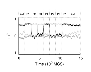
Figure 6: The same as in figure 5 but for three stored patterns that are orthogonal (instead of correlated). The stimulus is $+\delta\xi^{\nu},$ $\delta=0.1,$ with $\nu=\nu\left(t\right),$ as indicated at the top. The time evolution of the overlap $m^{\nu}$ is drawn with a different color (black, dark-grey and light-grey, respectively) for each value of $\nu$ to illustrate that the system keeps jumping between the patterns in this case.

The set of equations (4)–(6) provides a general framework to model activity–dependent processes. Motivated by the behavior of neurobiological systems, we adapted this to study the consequences of fast noise acting on the synapses of an attractor neural network with a finite number of stored patterns. We present in this paper two different scenarios corresponding to noise distributions fulfilling (9) and (19), respectively. In particular, assuming a local dependence on activity as in (17), one obtains the local fields (18), while a global dependence as in (20) leads to (23). Under certain assumptions, the system in the first of these cases is described by the effective Hamiltonian (8). This reduces to a Hopfield system —i.e., the familiar attractor neural network without any synaptic noise— with rescaled temperature and a threshold. This was already studied for a Gaussian distribution of thresholds [Hertz et al., 1991, Horn and Usher, 1989, Litinskii, 2002]. Concerning stationary properties, this case is also similar to the one in [Bibitchkov et al., 2002]. A more intriguing behavior ensues when the noise depends on the total presynaptic current arriving to the postsynaptic neuron. We studied this case both analytically, by using a mean–field hypothesis, and numerically by a series of Monte Carlo simulations using single-neuron dynamics. The two approaches are fully consistent with and complement each other.

Our model involves two main parameters. One is the temperature $T$ which controls the stochastic evolution of the network activity. The other parameter, $\Phi,$ controls the depressing noise intensity. Varying this, the system describes from normal operation to depression phenomena. A main result is that the presynaptic noise induces the occurrence of a tricritical point for certain values of these parameters, $(T_{c},\Phi_{c})=(1,-4/3).$ This separates (in the limit $\alpha\rightarrow 0$) first from second order phase transitions between a retrieval phase and a non–retrieval phase.

The principal conclusion in this paper is that fast presynaptic noise may induce a nonequilibrium condition which results in an important intensification of the network sensitivity to external stimulation. We explicitly show that the noise may turn unstable the attractor or fixed point solution of the retrieval process, and the system then seeks for another attractor. In particular, one observes switching from the stored pattern to the corresponding antipattern for $M=1,$ and switching between patterns for a larger number of stored patterns, $M.$ This behavior is most interesting because it improves the network ability to detect changing stimuli from the environment. We observe the switching to be very sensitive to the forcing stimulus, but rather independent of the network initial state or the thermal noise. It seems sensible to argue that, besides recognition, the processes of class identification and categorization in nature might follow a similar strategy. That is, different attractors may correspond to different objects, and a dynamics conveniently perturbed by fast noise may keep visiting the attractors belonging to a class which is characterized by a certain degree of correlation between its elements [Cortes et al., 2005]. In fact, a similar mechanism seems at the basis of early olfactory processing of insects [Laurent et al., 2001], and instabilities of the same sort have been described in the cortical activity of monkeys [Abeles et al., 1995] and other cases [Miller and Schreiner, 2000].

Finally, we mention that the above complex behavior seems confirmed by preliminary Monte Carlo simulations for a macroscopic number of stored patterns, i.e., a finite loading parameter $\alpha=M/N\neq 0.$ On the other hand, a mean–field approximation (see below) shows that the storage capacity of the network is $\alpha_{c}=0.138,$ as in the Hopfield case [Amit et al., 1987], for any $\Phi<0,$ while it is always smaller for $\Phi>0.$ This is in agreement with previous results concerning the effect of synaptic depression in Hopfield–like systems [Torres et al., 2002, Bibitchkov et al., 2002]. The fact that a positive value of $\Phi$ tends to shallow the basin thus destabilizing the attractor may be understood by a simple (mean–field) argument which is confirmed by Monte Carlo simulations [Cortes et al., 2005]. Assume that the stationary activity shows just one overlap of order unity. This corresponds to the condensed pattern; the overlaps with the rest, $M-1$ stored patterns is of order of $1/\sqrt{N}$ (non–condensed patterns) [Hertz et al., 1991]. The resulting probability of change of the synaptic intensity, namely, $\left(1+\alpha\right)\sum_{\nu=1}^{P}(m^{\nu})^{2}$ is of order unity, and the local fields (23) follow as $h_{i}^{\mathrm{eff}}\sim-\Phi h_{i}^{\mathrm{Hopfield}}.$ Therefore, the storage capacity, which is computed at $T=0,$ is the same as in the Hopfield case for any $\Phi<0,$ and always lower otherwise.

References

- [Abbott and Kepler, 1990] Abbott, L. F. and Kepler, T. B. (1990). Model neurons: From Hodgkin-Huxley to Hopfield. Lectures Notes in Physics, 368,5–18.
- [Abbott and Regehr, 2004] Abbott, L. F. and Regehr, W. G. (2004). Synaptic computation. Nature, 431,796–803.
- [Abeles et al., 1995] Abeles, M., Bergman, H., Gat, I., Meilijson, I., Seidelman, E., Tishby, N., and Vaadia, E. (1995). Cortical activity flips among quasi-stationary states. Proc. Natl. Acad. Sci. USA, 92,8616–8620.
- [Allen and Stevens, 1994] Allen, C. and Stevens, C. F. (1994). An evaluation of causes for unreliability of synaptic transmission. Proc. Natl. Acad. Sci. USA, 91,10380–10383.
- [Amari, 1972] Amari, S. (1972). Characteristics of random nets of analog neuron-like elements. IEEE Trans. Syst. Man. Cybern., 2,643–657.
- [Amit et al., 1987] Amit, D. J., Gutfreund, H., and Sompolinsky, H. (1987). Statistical mechanics of neural networks near saturation. Ann. Phys., 173,30–67.
- [Bibitchkov et al., 2002] Bibitchkov, D., Herrmann, J. M., and Geisel, T. (2002). Pattern storage and processing in attractor networks with short-time synaptic dynamics. Network: Comput. Neural Syst., 13,115–129.
- [Brunel and Hakim, 1999] Brunel, N., and Hakim, V. (1999). Fast Global Oscillations in Networks of Integrate-and-Fire Neurons with Low Firing Rates. Neural Comp., 11,1621–1671.
- [Cortes et al., 2005] Cortes, J. M., Garrido, P. L., Kappen, H. J., Marro, J., Morillas, C., Navidad, D., and Torres, J. J. (2005). Algorithms for identification and categorization. AIP Conf. Proc., In Press.
- [Cortes et al., 2004] Cortes, J. M., Garrido, P. L., Marro, J., and Torres, J. J. (2004). Switching between memories in neural automata with synaptic noise. Neurocomputing, 58-60,67–71.
- [Franks et al., 2003] Franks, K. M., Stevens, C. F., and Sejnowski, T. J. (2003). Independent sources of quantal variability at single glutamatergic synapses. J. Neurosci., 23(8),3186–3195.
- [Gardiner, 2004] Gardiner, C. W. (2004). Handbook of Stochastic Methods: for Physics, Chemistry and the Natural Sciences. Springer-Verlag.
- [Garrido and Marro, 1989] Garrido, P. L. and Marro, J. (1989). Effective Hamiltonian description of nonequilibrium spin systems. Phys. Rev. Lett., 62,1929–1932.
- [Garrido and Marro, 1991] Garrido, P. L. and Marro, J. (1991). Nonequilibrium neural networks. Lecture Notes in Computer Science, 540,25–32.
- [Garrido and Marro, 1994] Garrido, P. L. and Marro, J. (1994). Kinetic lattice models of disorder. J. Stat. Phys., 74,663–686.
- [Garrido and Munoz, 1993] Garrido, P. L. and Munoz, M. A. (1993). Nonequilibrium lattice models: A case with effective Hamiltonian in d dimensions. Phys. Rev. E, 48,R4153–R4155.
- [Hebb, 1949] Hebb, D. O. (1949). The Organization of Behavior: A Neuropsychological Theory. Wiley.
- [Hertz et al., 1991] Hertz, J., Krogh, A., and Palmer, R. (1991). Introduction to the theory of neural computation. Addison-Wesley.
- [Hopfield, 1982] Hopfield, J. J. (1982). Neural networks and physical systems with emergent collective computational abilities. Proc. Natl. Acad. Sci. USA, 79,2554–2558.
- [Horn and Usher, 1989] Horn, D. and Usher, M. (1989). Neural networks with dynamical thresholds. Phys. Rev. A, 40,1036–1044.
- [Lacomba and Marro, 1994] Lacomba, A. I. L. and Marro, J. (1994). Ising systems with conflicting dynamics: Exact results for random interactions and fields. Europhys. Lett., 25,169–174.
- [Laurent et al., 2001] Laurent, G., Stopfer, M., Friedrich, R. W., Rabinovich, M. I., Volkovskii, A., and Abarbanel, H. D. I. (2001). Odor encoding as an active, dynamical process: Experiments, computation and theory. Annu. Rev. Neurosci., 24,263–297.
- [Litinskii, 2002] Litinskii, L. B. (2002). Hopfield model with a dynamic threshold. Theoretical and Mathematical Physics, 130,136–151.
- [Marro and Dickman, 1999] Marro, J. and Dickman, R. (1999). Nonequilibrium Phase Transitions in Lattice Models. Cambridge University Press.
- [Marro et al., 1999] Marro, J., Torres, J. J., and Garrido, P. L. (1999). Neural network in which synaptic patterns fluctuate with time. J. Stat. Phys., 94(1-6),837–858.
- [Miller and Schreiner, 2000] Miller, L. M. and Schreiner, C. E. (2000). Stimulus-based state control in the thalamocortical system. J. Neurosci., 20,7011–7016.
- [Pantic et al., 2002] Pantic, L., Torres, J. J., Kappen, H. J., and Gielen, S. C. A. M. (2002). Associative memmory with dynamic synapses. Neural Comp., 14,2903–2923.
- [Pitler and Alger, 1992] Pitler, T. and Alger, B. E. (1992). Postsynaptic spike firing reduces synaptic gaba(a) responses in hippocampal pyramidal cells. J. Neurosci., 12,4122–4132.
- [Sompolinsky, 1986] Sompolinsky, H. (1986). Neural networks with nonlinear synapses and a static noise. Phys. Rev. A, 34,2571–2574.
- [Thomson et al., 2002] Thomson, A. M., Bannister, A. P., Mercer, A., and Morris, O. T. (2002). Target and temporal pattern selection at neocortical synapses. Philos. Trans. R. Soc. Lond. B Biol. Sci., 357,1781–1791.
- [Torres et al., 1997] Torres, J. J., Garrido, P. L., and Marro, J. (1997). Neural networks with fast time-variation of synapses. J. Phys. A: Math. Gen., 30,7801–7816.
- [Torres et al., 2004] Torres, J. J., Munoz, M. A., Marro, J., and Garrido, P. L. (2004). Influence of topology on the performance of a neural network. Neurocomputing, 58-60,229–234.
- [Torres et al., 2002] Torres, J. J., Pantic, L., and Kappen, H. J. (2002). Storage capacity of attractor neural networks with depressing synapses. Phys. Rev. E., 66,061910.
- [Tsodyks et al., 1998] Tsodyks, M. V., Pawelzik, K., and Markram, H. (1998). Neural networks with dynamic synapses. Neural Comp., 10,821–835.
- [Zador, 1998] Zador, A. (1998). Impact of synaptic unreliability on the information transmitted by spiking neurons. J. Neurophysiol., 79,1219–1229.