First passage times and asymmetry of DNA translocation

Abstract

Motivated by experiments in which single-stranded DNA with a short hairpin loop at one end undergoes unforced diffusion through a narrow pore, we study the first passage times for a particle, executing one-dimensional brownian motion in an asymmetric sawtooth potential, to exit one of the boundaries. We consider the first passage times for the case of classical diffusion, characterized by a mean-square displacement of the form $\left<(\Delta x)^{2}\right>\sim t$, and for the case of anomalous diffusion or subdiffusion, characterized by a mean-square displacement of the form $\left<(\Delta x)^{2}\right>\sim t^{\gamma}$ with $0<\gamma<1$. In the context of classical diffusion, we obtain an expression for the mean first passage time and show that this quantity changes when the direction of the sawtooth is reversed or, equivalently, when the reflecting and absorbing boundaries are exchanged. We discuss at which numbers of ‘teeth’ $N$ (or number of DNA nucleotides) and at which heights of the sawtooth potential this difference becomes significant. For large $N$, it is well known that the mean first passage time scales as $N^{2}$. In the context of subdiffusion, the mean first passage time does not exist. Therefore we obtain instead the distribution of first passage times in the limit of long times. We show that the prefactor in the power relation for this distribution is simply the expression for the mean first passage time in classical diffusion. We also describe a hypothetical experiment to calculate the average of the first passage times for a fraction of passage events that each end within some time $t^{\ast}$. We show that this average first passage time scales as $N^{2/\gamma}$ in subdiffusion.

I Introduction

Recent studies on the passage of DNA through narrow channels, apart from being very interesting in their own right, have been motivated by the exciting possibility of developing a practical technique to characterize and sequence DNA. These single molecule experiments were pioneered by Kasianowicz, Brandin, Branton and Deamer Kasianowicz using a protein called $\alpha$-hemolysin as a pore embedded in a lipid membrane. When voltage is applied across the membrane, ion current can be detected. When the DNA chain is inside and blocking the channel, the current is suppressed. By measuring the blockage time one can gather information about the voltage driven dynamics of DNA translocation. A large amount of exciting data have been accumulated through such experiments Akeson ; Meller1 ; Meller2 ; Meller3 . Recently, another group of experiments was performed using solid state nano-pores for voltage-driven DNA translocation Golovchenko ; Storm .

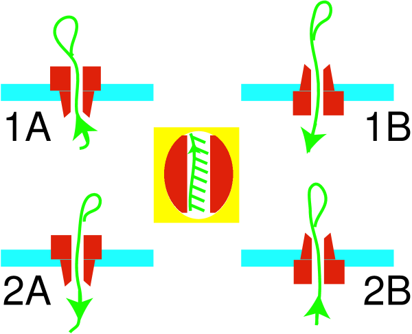
Figure 1: (Color online) The four possible relative orientations of DNA (“key”) and pore (“keyhole”). In a similar figure from Lubensky and Nelson (reference Lubensky , figure 7), the single-stranded DNA has no loop. Instead, the four cases were due to the various relative orientations of DNA, pore and an applied electric field. Arrows in our figure show the direction from the $5^{\prime}$ to the $3^{\prime}$ end in the DNA. Inset in the middle shows schematically the tilted bases. The analysis in our work compares the passage times for case 1A with case 1B (or 2A with 2B) in which the relative orientation between the DNA bases and pore is identical. In contrast, the experiments in Meller_explanation study cases 1A and 2A, where the DNA enters the pore from the same ($cis$) side.

On the theoretical side, much effort was placed in understanding the entropic barrier associated with translocation of a long polymer Park ; Muthukumar . The electrostatic barrier associated with charged DNA penetration through the low dielectric constant membrane has been recently discussed theoretically ZhangKamenevLarkinShklovskii . Another interesting question is about friction: whether friction on the small piece of DNA passing through the narrow channel is larger or smaller than the friction experienced by the large DNA coils outside the membrane. To this end, Lubensky and Nelson Lubensky , assuming the channel friction dominance, were able to account for the observed bimodal distribution of the passage times for single-stranded DNA. In their model, each base preferentially tilts towards one end of the single stranded DNA chain ($5^{\prime}$ or $3^{\prime}$. See figure 1.). Each peak in the distribution of passage times therefore corresponds to a particular end entering the channel first, the channel being just wide enough for a single strand to pass through. More recently, Kantor and Kardar KantorKardar and then Storm et al Storm argued that for sufficiently long DNA there must be a crossover to the regime of domination of the out-of-channel friction, in which case translocation should become subdiffusive in character (with displacement growing slower than $t^{1/2}$ with time $t$).

A new spin is added to the story by the experiment by Meller and coworkers Meller_explanation . These authors devised an experiment involving DNA having a string of identical bases (adenine) in the single-stranded portion and a hairpin loop at one end (figure 1) held in place by bonding of complementary bases. Like double-stranded DNA, the hairpin cannot enter the channel (a transmembrane pore of $\alpha$-Hemolysin). The hairpin therefore constrains the DNA to enter the pore with its single-stranded end, as well as preventing the entire DNA from crossing the membrane. In their experiment, the DNA, driven by an applied voltage, enters the pore with its single-stranded end. Thereafter, once current is blocked by the DNA, the voltage is either switched off, in which case the DNA diffuses freely (non-driven), or the sign of the voltage is flipped, in which case the DNA is pushed back. Moreover, by making two DNA samples, with the hairpin loop at opposite ends, it is possible to observe DNA sliding away from the pore in two opposite directions along the DNA contour, and the observation suggests that DNA escapes in one direction faster than in the other.

In the experiment Meller_explanation , by measuring the so-called “survival probability” $S(t)$, which is the probability that a DNA molecule will stay in the pore as a function of the waiting time, it was determined that the voltage-free dynamics of the $3^{\prime}$ threaded molecules is about two times slower than the corresponding diffusion of $5^{\prime}$ threaded molecules having the same sequence. Importantly, in both cases the DNA was threaded from the same side of the pore (called the $cis$-side of $\alpha$-HL). To delineate the underlying mechanism responsible for the observed dynamics, the authors of the work Meller_explanation performed all-atom molecular dynamics simulations, which independently confirmed the experimental results for driven DNA. The simulations also showed that the confinement of the DNA bases in the $\alpha$-HL pore results in an even stronger (compared to a free DNA) tilt of the bases with respect to the DNA backbone towards the $5^{\prime}$ end.

Authors of the work Meller_explanation phenomenologically interpret their data by assigning two different diffusion constants for the two separate experiments in which the same DNA is placed in the channel in two possible orientations. This interpretation is justified by the fact that the interactions between the DNA bases and the pore are different in these two cases (perhaps via different barrier heights within the framework of a sawtooth potential landscape discussed below).

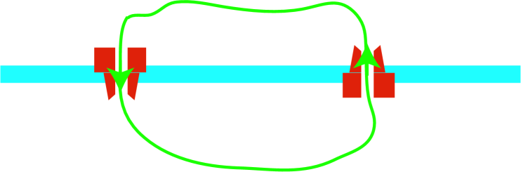
Figure 2: (Color online) This arrangement of DNA and pores would have acted as a perpetuum mobile if the stationary diffusion coefficient was asymmetric. This shows that it cannot be asymmetric, the symmetry being a requirement of thermodynamics.

There is a temptation to summarize the experimental findings of the work Meller_explanation in one sentence (although no one made this mistake, including Meller_explanation ): DNA diffuses in one direction faster than in the other. Indeed, the observed asymmetry of dynamics is consistent with the tilt of the nucleotides with respect to the main DNA chain. This asymmetry then seems easy to understand if the analogy is made with petting a cat along or against the grain of its fur; the cat responds very differently in the two cases (presumably because it experiences very different friction). Another, possibly even more obvious, analogy would be carrying a Christmas tree top first or base first through a narrow door; one again encounters very different resistance in the two cases. The point is that such analogies and interpretations are only possible for the driven DNA motion, particularly for the system far into the non-linear regime (in terms of force-velocity relation), whereas for the portion of experiments in the work Meller_explanation involving freely diffusing DNA such analogies and interpretations would be wrong; it is not surprising then that the authors of the work Meller_explanation did not use such analogies and interpretation for the freely diffusing DNA. Indeed, for free diffusion, the friction coefficient (averaged over the scale well exceeding a single base) moving in one direction and in the opposite direction must be the same, as follows from the Onsager symmetry relation, and the assumption of asymmetric friction would be a grave mistake. Although no one actually made this mistake, including Meller_explanation , it is worth emphasizing why an assumption of asymmetric friction would be a mistake. Indeed, if we only imagine that DNA (not driven by any applied voltage!) diffuses in one direction faster than in the other, then we can easily build a perpetuum mobile (see figure 2) moving indefinitely long through time at the expense of thermal energy from the thermal bath, which is, of course, impossible. In other words, freely diffusing DNA, when it is already in the pore, in contrast to a (heavily driven!) Christmas tree through a door, must have the same friction coefficients when the DNA moves in either direction.

What is nice is that the experimental findings and their interpretation in the work Meller_explanation are in fact in perfect agreement with this thermodynamic analysis. In order to make this reconciliation very clear, we immediately refer to the symmetry analysis in figure 1. Notice that the pore itself is asymmetric (its crystallographic structure is known structure ), the DNA backbone is also asymmetric (from $3^{\prime}$ end to $5^{\prime}$ end), and the loopy end creates further asymmetry. This gives four possible orientations of the pore and the DNA with the loop: two possibilities arise from two different mutual orientations of the DNA backbone with respect to the pore (indicated by the numbers 1 and 2 in figure 1), and for each of these two orientations there are two possibilities to place the blocking loop (indicated by the letters A and B in figure 1). This symmetry analysis, as shown in figure 1, is reminiscent of the symmetry analysis in the paper Lubensky , except we have no electric field, but instead have loops at the DNA ends.

We can now say that in any one of the arrangements, from 1A, 1B, 2A or 2B, the DNA must experience the same friction moving up or down the pore; friction going up equals friction going down. At the same time, the friction in configurations 1A or 1B can be different from friction in configurations 2A or 2B, and they are likely to be different. That is why the work Meller_explanation assigns two different diffusion constants to the two DNA-pore mutual configurations (1A and 2A). By contrast, the loop itself likely has no effect on the friction or diffusion coefficient, so we expect that the diffusion coefficient should be the same for configurations 1A and 1B (same goes for 2A and 2B). In other words, there should be two distinct diffusion coefficients, not four. We shall argue in this work that, nevertheless, there will be four different diffusion times corresponding to the four configurations in figure 1.

To explain our approach, it is convenient to adopt a terminology in which, instead of considering diffusion of the DNA chain, we consider diffusion of the passage point along the DNA contour. Following Lubensky and Nelson Lubensky , we consider a simple model in which asymmetry is presented in the underlying potential landscape. For simplicity, we model it with a sawtooth profile. The two orientations of the asymmetric potential (relative to the boundary conditions) correspond to the two possible placements of the blocking loop for a given orientation between DNA and pore (e.g. 1A and 1B in figure 1).

Like Lubensky and Nelson Lubensky , we focus on the first passage time, which is the time it takes for the initially fully-‘plugged’ DNA to completely ‘unplug’ from the pore. In other words, it is the time needed for the diffusing particle (or a random walker) to arrive for the first time on the open end of the DNA, or to one end of the $(0,L)$ interval, provided that a reflecting boundary condition is imposed at the opposite end.

We would like to emphasize the fundamental difference between asymmetric diffusion, which is prohibited by thermodynamics, and symmetric diffusion over the asymmetric potential landscape. It is well known, and we show it explicitly in appendix E, that stationary diffusion remains symmetric despite the asymmetry of the underlying potential landscape, thus making nonfunctional the perpetuum mobile design of figure 2.

In this paper, we compute the mean first passage times (MFPT) corresponding to cases 1A and 1B in figure 1 (or to cases 2A and 2B). We consider the brownian motion of a particle diffusing classically in an asymmetric sawtooth potential $U(x)$ and in the inverted or reversed version of the potential (figure 3). This model neglects the entropic barrier (of order $k_{B}T\ln N$) presented by the DNA coils on both sides of the pore Park ; Muthukumar , but through the consideration of subdiffusion it does take into account the extra friction created by those coils KantorKardar1 . From the results, we discuss when the difference between the two times is significant. (Note that since we know very little about the details of the interactions between the DNA bases and the pore, we cannot determine if case A in figure 3 corresponds to case 1A in figure 1, and case B in figure 3 corresponds to case 1B in figure 1, or if it is the other way around.)

Since DNA translocation is ultimately not classical diffusion, but rather subdiffusion Storm ; KantorKardar , we consider also the first passage times for the subdiffusion in the presence of an asymmetric potential. In general, the first passage time for subdiffusion was recently a matter of considerable interest and dispute in the literature Gitterman1 ; Yuste ; Gitterman2 . It is now understood WhenAnomalous ; Restaurant ; PhysicsWorld that the mean first passage time diverges for subdiffusion, because a subdiffusing walker tends to remain too long on the place that it once reached. Accordingly, we look at the probability distribution for the first passage times (DFPT), and concentrate on its tail at long times. We found that this tail is very different for the two potentials, and the difference turns out to be expressed through corresponding mean first passage times for classical diffusion. With this knowledge, we construct an average first passage time from a subset of passage events and show that this average scales as $N^{2/\gamma}$. The result also exhibits the asymmetry between cases 1A and 1B (or 2A and 2B) just as in the case of classical diffusion.

From our discussion we make the prediction that the observed passage times for the four possible mutual orientations of the pore and the DNA will all be different.

II Results

II.1 Classical diffusion

For treating classical or normal diffusion, one often starts with the Fokker-Planck (FPE) equation (in this context also frequently called Smoluchowsky equation)

$$\frac{\partial P(x,t)}{\partial t}=D\frac{\partial}{\partial x}e^{-U(x)}\frac{\partial}{\partial x}e^{U(x)}P(x,t)$$ (1)

giving the time-evolution of the probability density $P(x,t)$. Here $D$ is the usual diffusion constant and we have set $k_{B}T=1$. The FPE yields the Boltzmann distribution for $P$ in the steady-state, as well as giving the linear relation between the mean-squared displacement and time in the absence of external forces.

In calculations involving the first passage time, it would be convenient to consider the equivalent problem of first passage to either $x=L=Na$ or $x=-L=-Na$, where the potential $U(x)$ for $x>0$ is as illustrated in figure 3, while the potential for $x<0$ is $U(x)$ for positive $x$ reflected about the vertical axis. With this picture, the probability for the particle to still be ‘alive’ at time $t$, also called the survival probability $S(t)$ (and measured in experiment Meller_explanation ), is given by $S(t)=\int_{-L}^{L}P(x,t)dx$. The distribution of first passage times $F(t)$ is calculated from $S(t)$ via $F(t)=-\frac{\partial S(t)}{\partial t}$. This gives the following expression for the mean first passage time $\tau(x_{0})$ Redner :

$$\tau(x_{0}) = \int_{0}^{\infty}tF(t)dt$$ (2)

$$= \int_{0}^{\infty}S(t)dt$$

$$= \int_{0}^{\infty}\int_{-L}^{L}P(x,t)dxdt$$

where $x_{0}$ is the initial position of the particle, $P(x,0)=\delta(x-x_{0})$.

It can be shown that $\tau(x_{0})$ satisfies an ordinary differential equation Pontryagin ; FiftyYearsKramers ; Risken (derived in appendix B). The solution of this differential equation for a sawtooth potential $U(x)$ is outlined in appendix C. For the particle initially located at the origin ($x_{0}=0$), the mean first passage time to reach $x=L=Na$ is given by,

$$\tau_{A}=\alpha\frac{L^{2}}{2D}-\beta\frac{aL}{D}$$ (3)

for the potential in figure 3A, and

$$\tau_{B}=\alpha\frac{L^{2}}{2D}+\beta\frac{aL}{D}$$ (4)

for the potential in figure 3B. Here, we have defined the coefficients

$$\alpha = \left(\frac{\sinh{(U_{0}/2)}}{U_{0}/2}\right)^{2}$$ (5)

$$\beta = \frac{\sinh{(U_{0})}-U_{0}}{U_{0}^{2}}.$$ (6)

Expression (4) can be obtained from (3) by flipping the sign of $U_{0}$.

From the results (3) and (4), it is clear that $\tau_{A}<\tau_{B}$. Physically, the inequality $\tau_{A}<\tau_{B}$ may be obvious for the case $N=1$ in figure 3, in which a particle has to surmount a single barrier in order to get to $x=L$ in case B, while there is no barrier in case A. In general, for a given $N$, the potential in figure 3A involves $N-1$ barriers, while the potential in figure 3B involves $N$ barriers. In fact, it is easy to show that in the limit $U_{0}\gg 1$ ($U_{0}/k_{B}T\gg 1$ in more conventional units) we have $\tau_{A}(N+1)\simeq\tau_{B}(N)$, where the arguments indicate the number of teeth in the sawtooth potentials.

For the long DNA, when $L\gg a$ or $N\gg 1$, the leading terms in both $\tau_{A}$ (3) and $\tau_{B}$ (4) are proportional to $N^{2}$, as one would expect for diffusion times. To this leading order, first passage times $\tau_{A}$ and $\tau_{B}$ obey the symmetry in diffusion and are the same. It is in the subleading terms (proportional to $L$) that the two times differ. Let us stress that the difference between $\tau_{A}$ and $\tau_{B}$, which is of order of $1/N$ in a relative sense, is entirely due to the boundary conditions and the situation at the ends of the diffusion region.

II.2 Anomalous diffusion

Anomalous diffusion is characterized by the occurrence of a mean square displacement of the form $\left<(\Delta x)^{2}\right>\sim t^{\gamma}$, where $0<\gamma<1$ in subdiffusion; traditionally Metzler , this is written in the form

$$\left<(\Delta x)^{2}\right>=\frac{2D_{\gamma}}{\Gamma(1+\gamma)}t^{\gamma}$$ (7)

where $D_{\gamma}$ is a generalized diffusion constant and $\Gamma(x)$ is the gamma function. For $\gamma=1$ one recovers the usual result for classical diffusion. It can be shown Metzler that this form for the mean square displacement can be obtained from a generalized version of equation (1) called the fractional Fokker-Planck equation (FFPE). This equation is described in appendix A.

Although up to this point we have ignored the interactions of the DNA bases outside the pore, it seems reasonable to speculate that their effect is to slow down the translocation. Thus one might be able take these interactions into account phenomenologically by positing a value of $\gamma$ corresponding to the subdiffusive domain $0<\gamma<1$. (Reference WhenAnomalous lists possible sources of waiting time distributions leading to anomalous diffusion).

It is shown below and in references Yuste ; Gitterman2 ; WhenAnomalous ; Restaurant that the MFPT does not exist for subdiffusion. This leads us to consider the probability distributions themselves. The method of Laplace transforms can be used to solve for the transform of the survival probability Gitterman1 ; Gitterman2 but one is left with the very difficult task of obtaining the inverse transform, even for the case of a sawtooth with $N=1$. However, it is shown in appendix D that the long-time limit of the survival probability and the first passage time distribution scales as some power of $t$ and that they are simply related to the expression for the MFPT in the context of classical diffusion as follows

$$S(t)\sim\tau_{\gamma}\frac{t^{-\gamma}}{\Gamma(1-\gamma)}$$ (8)

$$F(t)=-\frac{\partial S(t)}{\partial t}\sim\tau_{\gamma}\frac{\gamma t^{-\gamma-1}}{\Gamma(1-\gamma)}$$ (9)

Here $\tau_{\gamma}$ is the same expression as the MFPT in classical diffusion (3) (or (4)), but containing a generalized diffusion constant. The long-time limit is reached when $t^{\gamma}\gg\tau_{\gamma}\sim L^{2}/D_{\gamma}\sim N^{2}$. The relationships (8) and (9) ultimately arise from the almost identical expressions for the solution $P(x,t)$ in classical diffusion and in subdiffusion. The two solutions differ only in the time dependence, which is an exponential for classical diffusion.

Because the expectation time of a first passage is infinite, any meaningful experiment, real or computational alike, must be based on some protocol rendering the observation time finite. We argue that in essence such a protocol is always reduced to discarding the events which fail to come to completion within some specified time $t^{\ast}$; in other words, only those passage events that each complete within some time $t^{\ast}$ are counted. The rest of the events that do not end by time $t^{\ast}$ are terminated and discarded. The conditional probability distribution of the first passage events that get counted under such a protocol is then given by

$$\frac{F(t)}{1-\int_{t^{\ast}}^{\infty}F(t)dt}$$ (10)

For such an experiment, there exists a perfectly defined and finite average first passage time. This conditional average, for large $t^{\ast}$, is

$$\frac{\int_{0}^{t^{\ast}}tF(t)dt}{1-\int_{t^{\ast}}^{\infty}F(t)dt} \sim \frac{\tau_{\gamma}\frac{\gamma{t^{\ast}}^{1-\gamma}}{(1-\gamma)\Gamma(1-\gamma)}}{1-\frac{\tau_{\gamma}}{{t^{\ast}}^{\gamma}\Gamma(1-\gamma)}}$$ (12)

$$\sim \tau_{\gamma}\frac{\gamma{t^{\ast}}^{1-\gamma}}{(1-\gamma)\Gamma(1-\gamma)}\times$$

$$\times\left(1+\frac{\tau_{\gamma}}{{t^{\ast}}^{\gamma}\Gamma(1-\gamma)}\right)$$

So far, the time $t^{\ast}$ should be long enough, but otherwise arbitrary. Now we argue that the time $t^{\ast}$ must be chosen such that roughly about half of the passage events at a given $N$ get discarded. This requirement seems reasonable, for if one discards a much smaller fraction $t^{\ast}$ becomes too large and the measurements get inefficiently slow; if one discards a much larger fraction $t^{\ast}$ becomes too small and the tail of the distribution does not get sampled properly. Thus, assuming half of the events discarded, $t^{\ast}$ becomes of order $(\tau_{\gamma})^{1/\gamma}$, just at the boundary of the validity of the asymptotics. Substituting this into (12), one obtains a scaling of $(\tau_{\gamma})^{1/\gamma}\sim N^{2/\gamma}$ for the average first passage time. Of course, this scaling is not unexpected for subdiffusion with an average displacement going like $t^{\gamma/2}$. Furthermore, due to the appearance of the classical diffusion times $\tau_{A}$ and $\tau_{B}$ (which take the place of $\tau_{\gamma}$ depending on the potential) in the average first passage time we just defined, the asymmetry of the first passage time is once again present in this case.

III Discussion

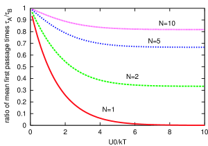
Figure 4: (Color online) The ratio $\tau_{A}/\tau_{B}$ plotted against the dimensionless drift or barrier height $va/D=U_{0}/k_{B}T$ for $N=1$ (bottommost curve), $N=2$, $N=5$ and $N=10$.

The ratio of the MFPTs in classical diffusion, expressions (3) and (4), is plotted in figure 4 for a few realistic values of $N$ and $U_{0}$. We see that for $U_{0}$ equal to a few $k_{B}T$, the difference becomes small ($\sim 10\%$) for $N>10$. For $N=50$, corresponding to the length of ssDNA used in the experiments by Meller and coworkers Meller_explanation , and for $U_{0}/k_{B}T\sim 10$, the fractional difference in MFPTs is about $4\%$ .

We emphasize again that one cannot use the results of the comparison between these two times (cases 1A and 1B in figure 1) and apply it to the experimental results in Meller_explanation (cases 1A and 2A in figure 1). Due to the asymmetry of the pore, the $3^{\prime}$ and the $5^{\prime}$ threading of DNA through one end of the pore (the so-called $cis$ side) cannot be readily reduced to cases 1A and 1B in figure 3.

Having established the difference in average first passage times for the two asymmetric potentials, let us now turn to the scaling of the first passage times with $N$. For large $N$, the scaling result $N^{2}$ found earlier is well known for classical diffusion or Brownian dynamics. However, this is in conflict with the equilibration time of a polymer with $N$ monomers in the absence of a pore and membrane, which already scales with $N$ to some power larger than $2$ for Rouse dynamics of self-avoiding chains KantorKardar1 . This suggests that a correct description of polymer translocation should be made in the context of subdiffusion, where the scaling of the average first passage time is to power $1/\gamma>1$ of the classical result, although we do not give a prediction for the value of $\gamma$ itself because the interactions involving the DNA/polymer located outside the pore were not treated explicitly. The scaling $N^{2/\gamma}$ is also not surprising if one takes the relation $\left<(\Delta x)^{2}\right>\sim t^{\gamma}$ and puts $\Delta x\sim N$, but it does not rule out the argument made above regarding $t^{\ast}$, only that it gives a reasonable and somewhat expected answer. Moreover, using similar arguments, the result $N^{2/\gamma}$ is consistent with numerical simulations made by Chuang, Kantor and Kardar KantorKardar1 for diffusive dynamics of self-avoiding chains in two dimensions. They found that the average of the first passage time scales as $\tau\sim N^{2.5}=N^{1+2\nu}$, where $\nu=3/4$ in two dimensions. They also argued, assuming that the translocation coordinate goes like $\left<\Delta x^{2}(t)\right>\sim t^{\gamma}$ at short times, that $\gamma=2/(1+2\nu)$. Eliminating $\nu$, their formulas imply that $\tau\sim N^{2/\gamma}$.

To summarize, based on our calculations for the mean first passage times in asymmetric sawtooth potentials and experiments by Meller and coworkers Meller_explanation , we expect that the average first passage times for the four cases indicated in figure 1 are all different. The expression for the tail of the first passage time distribution in subdiffusion is of the form $\gamma\tau_{\gamma}/\Gamma(1-\gamma)t^{1+\gamma}$, where $\tau_{\gamma}$ is the formula for the mean first passage time in classical diffusion. Because the power of $t$ in the distribution is less than two, the mean first passage time diverges. By constructing an average from the first passage times less than time $t^{\ast}$ such that approximately half of the passages get rejected, we find an average that scales as $(\tau_{\gamma})^{1/\gamma}\sim N^{2/\gamma}$.

IV Acknowledgments

This work was inspired by an interesting seminar talk given by Amit Meller. We also acknowledge useful subsequent discussions with him. RCL acknowledges the support of a doctoral dissertation fellowship from the University of Minnesota graduate school. We also wish to thank the Minnesota Supercomputing Institute for the use of their facilities. This work was supported in part by the MRSEC Program of the National Science Foundation under Award Number DMR-0212302.

Appendix A Fractional Fokker-Planck equation

A generalization of the FPE describing anomalous diffusion is given by the fractional FPE Metzler

$$\frac{\partial P(x,t)}{\partial t}=\ _{0}D^{1-\gamma}_{t}L_{\mbox{FP}}P$$ (13)

Equivalently,

$$\ {}_{0}D^{\gamma}_{t}P(x,t)-\frac{t^{-\gamma}P(x,0)}{\Gamma(1-\gamma)}=L_{\mbox{FP}}P$$ (14)

where the Fokker-Planck operator is defined as

$$L_{\mbox{FP}}=D_{\gamma}\frac{\partial}{\partial x}e^{-U(x)}\frac{\partial}{\partial x}e^{U(x)}$$ (15)

Here $D_{\gamma}$ is a generalized diffusion coefficient and $U(x)$ is an external potential. We have also set $k_{B}T=1$ and the Einstein relation is implicit. The Riemann-Liouville fractional operator is defined through

$$\ {}_{0}D^{1-\gamma}_{t}W=\frac{1}{\Gamma(\gamma)}\frac{\partial}{\partial t}\int_{0}^{t}dt^{\prime}\frac{W(x,t^{\prime})}{(t-t^{\prime})^{1-\gamma}}\ .$$ (16)

One can easily check that the FFPE reduces to the FPE or diffusion equation for $\gamma=1$.

Given the initial distribution $P(x,0)=\delta(x-x_{0})$, the solution to equation (13) is given by the bilinear expansion Metzler

$$P(x,t;x_{0},0) = e^{U(x_{0})/2-U(x)/2}\times$$ (17)

$$\times \sum_{n=0}^{\infty}\psi_{n}(x)\psi_{n}(x_{0})E_{\gamma}(-\lambda_{n}t^{\gamma})\ .$$

The functions $\phi_{n}(x)=e^{-U(x)/2}\psi_{n}(x)$ and $T_{n}(t)=E_{\gamma}(-\lambda_{n}t^{\gamma})$ appear in the separation of variables ansatz $W_{n}(x,t)=\phi_{n}(x)T_{n}(t)$. The product function $W_{n}(x,t)$ satisfies the FFPE. Note that the coordinate dependence comes through the eigenfunctions $\psi_{n}(x)$ or $\phi_{n}(x)$, which are the same as for regular diffusion, satisfying the (eigenvalue) equations

$$L_{\mbox{FP}}\phi_{n}(x)=-\lambda_{n}\phi_{n}(x)\ ,$$ (18)

$$L^{hermitian}_{\mbox{FP}}\psi_{n}(x)=-\lambda_{n}\psi_{n}(x)\ ,$$ (19)

$$L^{hermitian}_{\mbox{FP}}=e^{U(x)/2}L_{\mbox{FP}}e^{-U(x)/2}\ .$$ (20)

However, as to the time dependence, which for classical diffusion is described by exponentials ($e^{-\lambda_{n}t}$), for subdiffusion it must satisfy the equation

$$\frac{dT_{n}(t)}{dt}=-\lambda_{n}\ {}_{0}D^{\gamma}_{t}T_{n}(t)\ .$$ (21)

One can check that the following series definition of the Mittag-Leffler function $E_{\gamma}(z)$ satisfies equation (21)

$$E_{\gamma}(z)=\sum_{m=0}^{\infty}\frac{z^{m}}{\Gamma(1+\gamma m)}\ .$$ (22)

This function is a natural extension of the exponential function, to which it degenerates for $\gamma=1$.

By taking the Laplace transform of both sides of equation (21), one obtains an alternative definition of the Mittag-Leffler function

$${\cal L}\left\{E_{\gamma}(-\lambda t^{\gamma})\right\}=\left(s+\lambda s^{1-\gamma}\right)^{-1}$$ (23)

(The subscript in the constant $\lambda$ has been dropped.) The long-time limit of the Mittag-Leffler function corresponds to the small $s$ limit of the Laplace transform. Expanding (23) in a series for small $s$,

$${\cal L}\left\{E_{\gamma}(-\lambda t^{\gamma})\right\} \sim \frac{1}{\lambda s^{1-\gamma}}\left(1-\frac{s^{\gamma}}{\lambda}+\left(\frac{s^{\gamma}}{\lambda}\right)^{2}-\cdots\right)$$ (24)

$$\sim \sum_{m=1}^{\infty}(-1)^{m+1}\frac{s^{\gamma m-1}}{\lambda^{m}}$$

Taking the inverse transform, one obtains the long-time behaviour of the Mittag-Leffler function

$$E_{\gamma}(-\lambda t^{\gamma})\sim\sum_{m=1}^{\infty}\frac{(-1)^{m+1}}{\Gamma(1-\gamma m)}\left(\lambda t^{\gamma}\right)^{-m}$$ (25)

For $\epsilon=1-\gamma=0$, the Laplace transform (23) becomes $(s+\lambda)^{-1}$, the inverse transform of which is an exponential. For $\epsilon$ close to $0$, we expect a long time interval in which the behaviour of the Mittag-Leffler function $E_{\gamma}(-\lambda t^{\gamma})$ behaves like an exponential; at much longer times the behaviour changes to a power law. The crossover is expected to happen when $e^{-\lambda t_{c}}\sim\frac{1}{\Gamma(\epsilon)\lambda t_{c}^{\gamma}}$, or at about $t_{c}\sim\frac{1}{\lambda}\ln(\frac{1}{\epsilon})$.

Appendix B Differential equation satisfied by the mean first passage time

Recall that the MFPT can be calculated from (equation (2))

$$\tau(x_{0})=\int_{0}^{\infty}\int_{-L}^{L}P(x,t)dxdt$$ (26)

To derive an ordinary differential equation satisfied by $\tau(x_{0})$, apply the operator $e^{U(x_{0})}L_{\mbox{FP},x_{0}}e^{-U(x_{0})}$ to equation (26) and use the eigenfunction expansion solution (17) for $P(x,t)$,

$$e^{U(x_{0})}L_{\mbox{FP},x_{0}}e^{-U(x_{0})}\tau(x_{0}) = \int_{0}^{\infty}\int_{-L}^{L}e^{U(x_{0})/2-U(x)/2}\sum_{n=0}^{\infty}(-\lambda_{n})\psi_{n}(x)\psi_{n}(x_{0})E_{\gamma}(-\lambda_{n}t^{\gamma})dxdt$$

$$= \int_{0}^{\infty}\int_{-L}^{L}L_{\mbox{FP}}P(x,t)dxdt=\int_{0}^{\infty}\int_{-L}^{L}\left[\ {}_{0}D^{\gamma}_{t}P(x,t)-\frac{t^{-\gamma}P(x,0)}{\Gamma(1-\gamma)}\right]dxdt$$

In the last two steps, the eigenvalue equations and the second version of the FFPE (equation (14)) was used.

Using the initial condition $P(x,0)=\delta(x-x_{0})$ and the definition of the fractional operator, after some algebra one obtains

$$e^{U(x_{0})}L_{\mbox{FP},x_{0}}e^{-U(x_{0})}\tau(x_{0})=$$

$$-\lim_{t\rightarrow\infty}\left[\frac{t^{1-\gamma}}{\Gamma(2-\gamma)}-\frac{1}{\Gamma(1-\gamma)}\int_{0}^{t}\frac{S(t^{\prime})}{(t-t^{\prime})^{\gamma}}dt^{\prime}\right]$$ (27)

or

$$D_{\gamma}e^{U(x_{0})}\frac{\partial}{\partial x_{0}}e^{-U(x_{0})}\frac{\partial}{\partial x_{0}}\tau(x_{0})=$$

$$-\lim_{t\rightarrow\infty}\left[\frac{t^{1-\gamma}}{\Gamma(2-\gamma)}-\frac{1}{\Gamma(1-\gamma)}\int_{0}^{t}\frac{S(t^{\prime})}{(t-t^{\prime})^{\gamma}}dt^{\prime}\right]$$ (28)

For $\gamma=1$, corresponding to classical diffusion, the survival probability $S(t^{\prime})$ decays exponentially and the term with the integral goes to zero, yielding the familiar result of $-1$ for the right-hand-side Pontryagin ; FiftyYearsKramers ; Risken . For $\gamma<1$, $S(t^{\prime})$ goes like $(t^{\prime})^{-\gamma}$ (see (33)) and the term with the integral goes like $t^{1-2\gamma}$. The right-hand-side diverges, which hints at the non-existence of the MFPT for subdiffusion Yuste ; Gitterman2 ; WhenAnomalous ; Restaurant ; PhysicsWorld .

Appendix C Solution for the mean first passage time in a sawtooth potential

From the previous section, the differential equation satisfied by the MFPT in the context of classical diffusion is (temporarily putting back $k_{B}T$)

$$De^{U(x)/k_{B}T}\frac{d}{dx}e^{-U(x)/k_{B}T}\frac{d\tau(x)}{dx}=-1$$ (29)

We solve for $\tau(x)$ in this equation for a sawtooth potential (case A, figure 3) subject to the boundary conditions $d\tau/dx(0)=0$ and $\tau(L)=0$, and the continuity of $\tau$ and $e^{-U/k_{B}T}d\tau/dx$ in $(0,L)$. In what follows we let $\xi=e^{va/D}=e^{U_{0}/k_{B}T}$.

The solution, for $x$ between $(m-1)a$ and $ma$ where $m$ is an integer between $1$ and $N$ (inclusive), is given by

$$\tau(x)=A_{m}e^{-vx/D}-\frac{x}{v}+B_{m}$$ (30)

The coefficients $A$ and $B$ are given by

$$A_{m} = \xi^{m-1}\frac{D}{v^{2}}\left[(\xi-1)(m-1)-1\right]\ ;$$

$$B_{m} = \frac{D}{v^{2}}+N\left(\frac{a}{v}-(1-1/\xi)\frac{D}{v^{2}}\right)+$$ (31)

$$+ \frac{D}{v^{2}}\frac{(\xi-1)^{2}}{\xi}\frac{(N-m)(N+m-1)}{2}\ .$$

The MFPT for a particle initially located at $x=0$ is given by $\tau(0)=A_{1}+B_{1}$. To obtain the solution for case B in figure 3, we may flip $\xi$ ($\rightarrow 1/\xi$) and the sign of $v$ in the expressions above.

Appendix D Relationship between the DFPT in anomalous diffusion and the MFPT in classical diffusion

Since the MFPT does not exist for subdiffusion, one would want to calculate the distributions instead. In the long time limit, using (17) and (25),

$$\lim_{t\rightarrow\infty}P_{\gamma}(x,t;x_{0},0)\sim\sum_{n}e^{U(x_{0})/2-U(x)/2}\psi_{n}(x)\psi_{n}(x_{0})\frac{1}{\Gamma(1-\gamma)\lambda_{n}t^{\gamma}}$$ (32)

$$\lim_{t\rightarrow\infty}S_{\gamma}(t)\sim\sum_{n}\left(\int_{-L}^{L}e^{-U(x)/2}\psi_{n}(x)dx\right)e^{U(x_{0})/2}\psi_{n}(x_{0})\frac{1}{\Gamma(1-\gamma)\lambda_{n}t^{\gamma}}$$ (33)

$$\lim_{t\rightarrow\infty}F_{\gamma}(t)\sim\sum_{n}\left(\int_{-L}^{L}e^{-U(x)/2}\psi_{n}(x)dx\right)e^{U(x_{0})/2}\psi_{n}(x_{0})\frac{\gamma}{\Gamma(1-\gamma)\lambda_{n}t^{\gamma+1}}$$ (34)

Again, these results indicate that the MFPT diverges for $\gamma<1$. It is also interesting to note that all the eigenfunctions $\psi_{n}(x)$, not just the ground state, enter in the expressions.

To make sense of the expression multiplying $\frac{\gamma}{\Gamma(1-\gamma)t^{\gamma+1}}$ in (34) write down the corresponding solution for classical diffusion under the same potential and the same value for the diffusion coefficient

$$P(x,t;x_{0},0) = e^{U(x_{0})/2-U(x)/2}\times$$ (35)

$$\times \sum_{n=0}^{\infty}\psi_{n}(x)\psi_{n}(x_{0})\exp(-\lambda_{n}t)$$

(Note exponential instead of Mittag-Leffler function). The survival probability is given by

$$S(t) = \sum_{n}\left(\int_{-L}^{L}e^{-U(x)/2}\psi_{n}(x)dx\right)\times$$ (36)

$$\times e^{U(x_{0})/2}\psi_{n}(x_{0})\exp(-\lambda_{n}t)$$

While the MFPT is given by

$$\tau(x_{0}) = \int_{0}^{\infty}S(t)dt$$ (37)

$$= \sum_{n}\left(\int_{-L}^{L}e^{-U(x)/2}\psi_{n}(x)dx\right)\times$$

$$\times e^{U(x_{0})/2}\psi_{n}(x_{0})\frac{1}{\lambda_{n}}$$

which is identical to the coefficient of $\gamma\left/\Gamma(1-\gamma)t^{\gamma+1}\right.$ in (34).

Appendix E Effective diffusion constant in the steady state

In this section we determine the steady state current $J$ given fixed concentrations $c(0)$ and $c(L)$ at the boundaries. Let the potential $U(x)$ satisfy $U(0)=U(L)=0$, but is otherwise arbitrary. The classical diffusion equation is given by

$$\frac{\partial c}{\partial t}=-\frac{\partial J}{\partial x}$$ (38)

where $J=-De^{-U(x)}\frac{\partial}{\partial x}e^{U(x)}c$ (see equation (1)). In the steady state, $\frac{\partial c}{\partial t}=0$, which implies that $J$ is spatially uniform. Integrating $Je^{U(x)}=-D\frac{\partial}{\partial x}e^{U(x)}c(x)$ and utilizing the boundary conditions, one obtains

$$J=\frac{D}{\int_{0}^{L}e^{U(x)}dx}(c(0)-c(L))\ .$$ (39)

This expression is identical with Fick’s law with an effective diffusion constant of $\frac{DL}{\int_{0}^{L}e^{U(x)}dx}$.

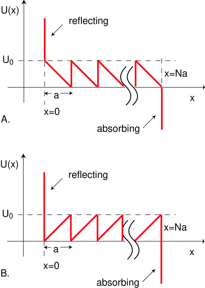
Figure 3: (Color online) The sawtooth potential of $N$ teeth with a reflecting boundary at $x=0$ and an absorbing boundary at $x=L=Na$, illustrated for two different directions of asymmetry in the sawtooth. The reflecting boundary corresponds to the inability of the DNA hairpin to pass through the pore.

References

- (1) J.J. Kasianowicz, E. Brandin, D. Branton, and D.W. Deamer, Proc. Natl. Acad. Sci. U.S.A. 93, 13770 (1996).
- (2) M. Akeson, D. Branton, J.J. Kasianowicz, E. Brandin, and D.W. Deamer, Biophys. J. 77, 3227 (1999).
- (3) A. Meller, L. Nivon, E. Brandin, J. Golovchenko, and D. Branton, Proc. Natl. Acad. Sci. U.S.A. 97, 1079 (2000).
- (4) A. Meller and D. Branton, Electrophoresis 23, 2583 (2002).
- (5) A. Meller, L. Nivon, and D. Branton, Phys. Rev. Lett. 86, 3435 (2001).
- (6) J.L. Li, M. Gershow, D. Stein, E. Brandin, and J. A. Golovchenko, Nat. Mater. 2, 611 (2003).
- (7) A.J. Storm, C. Storm, J. Chen, H. Zandbergen, J.F. Joanny, and C. Dekker, Nano Lett. 5, 1193 (2005).
- (8) W. Sung and P.J. Park, Phys. Rev. Lett. 77, 783 (1996).
- (9) M. Muthukumar, J. Chem Phys. 111, 10371 (1999).
- (10) A. Kamenev, J. Zhang, A.I. Larkin and B.I. Shklovskii, eprint arXiv:cond-mat/0503027.
- (11) D.K. Lubensky and D.R. Nelson, Biophys. J. 77, 1824 (1999).
- (12) Y. Kantor and M. Kardar, Phys. Rev. E 69, 021806 (2004).
- (13) J. Chuang, Y. Kantor, and M. Kardar, Phys. Rev. E 65, 011802 (2002).
- (14) J. Mathe, A. Aksimentiev, D.R. Nelson, K. Schulten and A. Meller, Proc. Natl. Acad. Sci. U.S.A. 102, 12377 (2005).
- (15) L. Song, M.R. Hobaugh, C. Shustak, S. Cheley, H. Bayley, J.E. Gouaux, Science 274, 1859-1866 (1996).
- (16) M. Gitterman, Phys. Rev. E 62, 6065 (2000).
- (17) S.B. Yuste and K. Lindenberg, Phys. Rev. E 69, 033101 (2004).
- (18) M. Gitterman, Phys. Rev. E 69, 033102 (2004).
- (19) R. Metzler and J. Klafter, Biophys. J. 85, 2776 (2003).
- (20) R. Metzler and J. Klafter, J. Phys. A: Math. Gen. 37, R161 (2004).
- (21) J. Klafter and I. Sokolov, Physics World, August issue, 29 (2005).
- (22) R. Metzler, E. Barkai, and J. Klafter, Phys. Rev. Lett. 82, 3563 (1999).
- (23) L. Pontryagin, A. Andronov, and A. Vitt, Zh. Eksp. Teor. Fiz. 3, 165 (1933); translated and reprinted in Noise in Nonlinear Dynamical Systems, Vol. 1, edited by F. Moss and P. V. E. McClintock (Cambridge Univ. Press, Cambridge, in press), p. 329.
- (24) P. Hänggi, P. Talkner and M. Borkovec, Rev. Mod. Phys. 62, 251 (1990).
- (25) S. Redner, A Guide to First-Passage Processes (Cambridge University Press, Cambridge, 2001).
- (26) H. Risken, The Fokker-Planck Equation (Springer-Verlag, Berlin, 1984).