onlysubmission\excludeversiononlypreprint \includeversionnowordcount
Food Webs: Experts Consuming Families of Experts
The question what determines the structure of natural food webs has been listed among the nine most important unanswered questions in ecology may99:_unansered. It arises naturally from many problems related to ecosystem stability and resilience mccann00:_diversity_stability_review; yodzis98:_local_benguel_interactions. The traditional yodzis81:stability_real_ecosystems view is dunne05:_model_complex_stab that population-dynamical stability is crucial for understanding the observed camacho02:_robus_patter_food_web_struc; milo02:_networ_motif; neutel02:_stabil_real_food_webs; williams00:_simpl; cattin04:_phylog; cohen90:_commun_food_webs_AND_THEREIN structures. But phylogeny (evolutionary history) has also been suggested cattin04:_phylog as the dominant mechanism. Here we show that observed topological features of predatory food webs can be reproduced to unprecedented accuracy by a mechanism taking into account only phylogeny, size constraints, and the heredity of the trophically relevant traits of prey and predators. The analysis reveals a tendency to avoid resource competition rather than apparent competition holt94:_ecolog_conseq_shared_natur_enemies. In food webs with many parasites morris01:_field_apparnt_comp this pattern is reversed.
Empirical food-web data is notorious for its inhomogeneity cohen93:_improving_food_webs. In particular, the large number of species interacting in habitats has forced researchers to disregard whole subsystems or to coarsen the taxonomic resolution cohen90:_commun_food_webs_AND_THEREIN. The representation of trophic interactions by the simple absence or presence of links in topological food webs is problematic, because it turns out that by various measures berlow04:_interac_strength weak links are more frequent than strong links in natural food webs, and network structures depend on a somewhat arbitrary thresholding among the weak links martinez99:_effec_sampl_effor_charac_food_web_struc; wilhelm03:_elementary_dyn_mod. Furthermore, the use of different methods for determining links cohen93:_improving_food_webs might affect the result. Our analysis takes these difficulties into account by employing a quantitative link-strength concept, an appropriate data standardization (see Supplementary Methods), and by reflecting the inhomogeneity of empirical methodology in our food-web model and data analysis.
Specifically, the following model (“matching model”) describing the evolution of an abstract species pool is employed: The foraging and vulnerability traits of each species caldarelli98:_model_multispec_commun; drossel01:_influen_predat_prey_popul_dynam; yoshida03:_dynam_web_model are modeled by two sequence of ones and zeros of length (the reader might think of oppositions such as sessile/vagile, nocturnal/diurnal, or benthic/pelagic). The strength of trophic links increases (nonlinearly) with the number of foraging traits of the consumer that match the corresponding vulnerability traits of the resource (Figure 1). A trophic link is considered as present if the number of matched traits exceeds some threshold . In addition, each species is associated with a size parameter characterizing the (logarithmic) body size of a species (). Consumers cannot forage on species with size parameters larger than their own by more than . The model parameter () controls the amount of trophic loops polis91:_compl_des_web in a food web.
The complex processes driving evolution are modeled by speciations and extinctions that occur for each species randomly at rates and , respectively raup91:_phaner_kill. New species invade the habitat at a rate . Such continuous-time birth-death processes are well understood bailey64:_stoch_proces_CHAP_8_7. With the steady-state average of the number of species is . For new, invading species the traits and the size parameter are determined at random with equal probabilities. For the descendant species of a speciation (Figure 1), each vulnerability trait is flipped with probability , each foraging trait is flipped with probability , and a zero-mean Gaussian random number () is added to the size parameter of the predecessor ( are treated as reflecting boundariesrossberg05:_spec). Such a random, undirected model of macroevolution becomes plausible if one assumes the trophic niche space to be in a kind of “occupation equilibrium”: there are no large voids in niche space to be filled and no niche-space regions of particularly strong predation pressure to avoid.
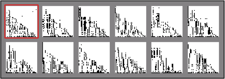
The model has the adjustable parameters , , , , , , , and . For large food-web dynamics become independent of , provided is adjusted such as to keep the probability for link strengths to exceed the threshold constant (Supplementary Discussion). Throughout this work is used. Figure 2 and Supplementary Figures 2-18 display the connection matrices of randomly sampled steady-state model webs in comparison with empirical data; a Supplementary Movie illustrates the model dynamics.
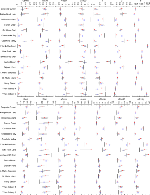
The model was validated by comparing snapshots of the steady state with empirical data. Thus, only the relative evolution rates and matter. We set . The size-dispersion constant has only a weak effect on results (for not too large , , only the ratio is relevantrossberg05:_spec, as we verified numerically for ) and was kept fixed at . The remaining six parameters , , , , , and were chosen such as to fit 14 ecologically relevant, quantitative food-web properties to empirical data (Supplementary Figure 1), separately for each of 17 well-studied data sets (maximum likelihood fits, see Supplementary Methods for properties, sources of food-web data, and fitting procedure). Results are listed in Table 1. Each fitted parameter set required statistically independent Monte-Carlo simulations.
To quantify the goodness-of-fit we computed statistics (Supplementary Methods) corresponding to the remaining statistical degrees of freedom (DOF) for each data set (Table 1, ). Not all empirical food-webs are fitted equally well. For the three food webs labeled Scotch Broom, British Grassland, and Ythan Estuary 2 the value of exceeds the Bonferroni-corrected -confidence interval (15 webs). Discrepancies between the remaining 14 data sets and the model, on the other hand, are revealed only when pooling all 14 sets: for gives .
For comparisons, the niche model williams00:_simpl (one of the best description known so far) was fitted to the data using the same procedure (Supplementary Methods), and the differences of the Akaike Information Criterion for fits to the matching model () and the niche model () were computed. This statistic takes the fact into account that the matching model is more complex and contains four parameters more than the niche model. Negative indicate that the matching model describes the data better than the niche model and the increased model complexity is justified. The value is negative for 12 out of 17 models. In the cases where this is due to unnecessary complexity of the matching model, and not due to a better fit of the niche model, as a comparison of the corresponding values (Table 1, niche model: ) shows. Pooling all data yields in favor of the matching model. A comparison of the nested hierarchy model cattin04:_phylog; rossberg05:_web; stouffer05:_quant_patterns_webs with our model gives similar results ().
Among the fitted model parameters some depend just as much on methodological choices at the time of recording the food web as on the actual ecology. In particular the linking probability directly corresponds to the threshold for link assignment, and the invasion rate —as a parameter determining the web size—depends on the delineation of the habitat and the species-sampling effort. The degree of loopiness might depend on the particular method used to determine links empirically. Adjusting these three parameters makes the model robust to differences in empirical methodology.
The remaining three parameters , , and allow, at least partially, an ecological interpretation. represents the fraction of species that entered the species pool by speciations from other species in the pool, in contrast to the remaining that entered through random “invasions”. The low values found for (Table 1) indicate that evolutionary processes are essential for generating the observed structures.
The two quantities and measure the variability of vulnerability and foraging traits among related species. We typically find much smaller than (Table 1). In particular, in 14 of 17 data sets (). This implies that descendant species tend to acquire resources sets different from their ancestors but mostly share their enemies. We interpret this as a preference for avoiding resource competition rather than apparent competition holt94:_ecolog_conseq_shared_natur_enemies: A typical consumer is an expert for its particular set of resources (resource partitioning), and a typically resource set consists of a few “families” of related species—autotrophs or, again, expert consumers.
The three exceptional data sets with are exactly those most difficult to fit by the matching model (Table 1). Interestingly, these are also the three data sets that contain large fractions () of parasites, parasitoids, and pathogens (PPP) in the resolved species pool. The other data sets are dominated by predators, grazers, and primary produces (PPP fraction ). These observations are consistent with the expectations that (i) due to their high specialization PPP are less susceptible to resource competition than predators morris01:_field_apparnt_comp and (ii) the matching model does not describe PPP well because it assumes a size ordering which is typical only for predator-prey interactions warren87:_pre_pry_triang; cohen93:_body_size; memmott00:_predat_size_web; warren89:_spatial_freshw_web. But further investigations of these points are required. For example, contrary to expectations, is close to one also for Ythan Estuary 1.
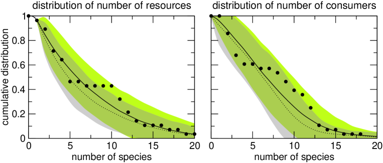
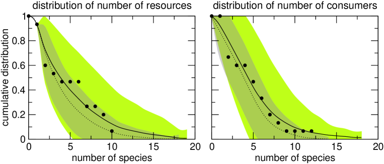
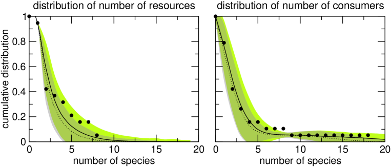
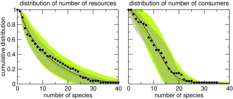
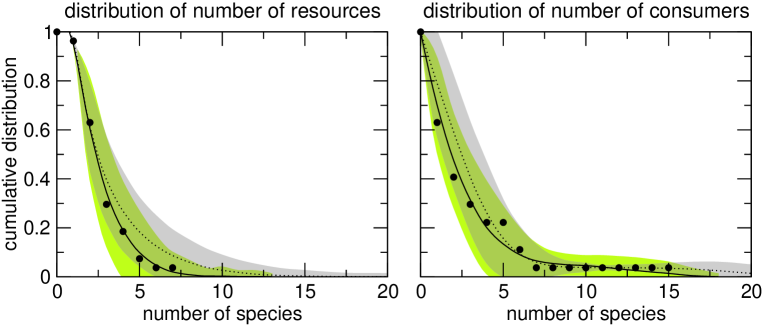
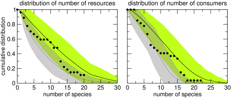
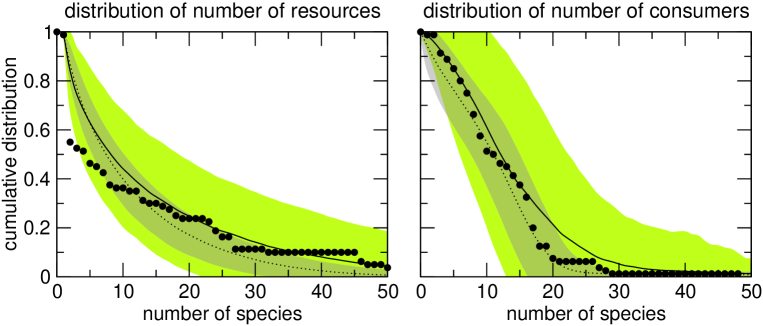
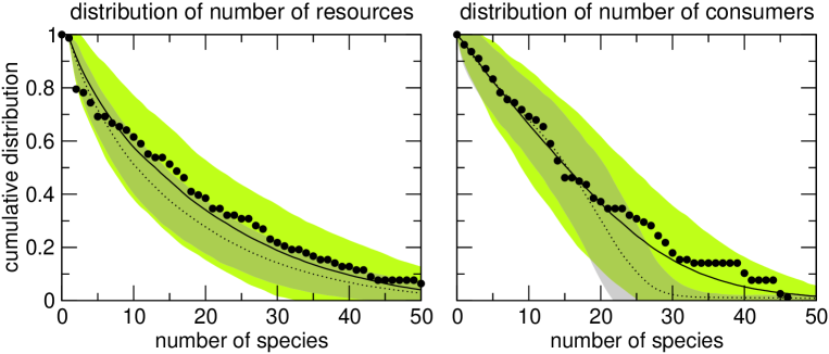
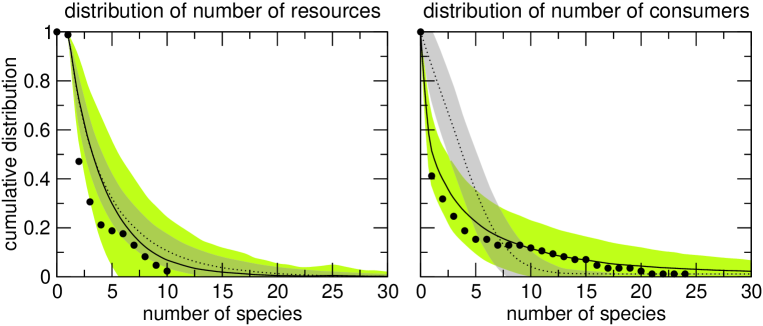
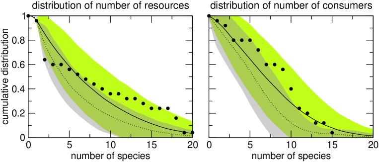
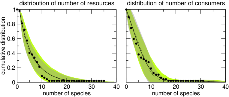
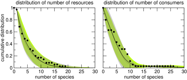
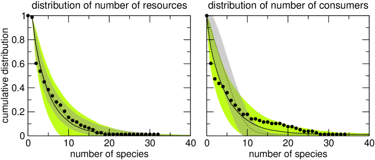
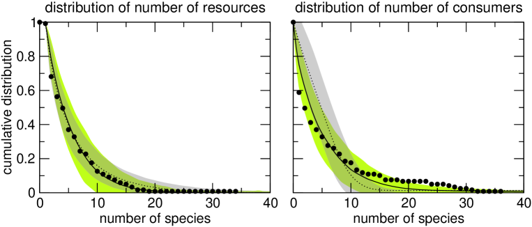
The matching model reproduces the empirical distributions of the numbers of consumers and resources of species well (Figure 3, Supplementary Figures 2-18). Under specific conditions (see Supplementary Discussion)—including —these become the “universal”, scaling distributions camacho02:_robus_patter_food_web_struc; stouffer05:_quant_patterns_webs characteristic for the niche model (e.g., Figure 3, Caribbean Reef). But the distributions for food webs deviating from these patterns are also reproduced (e.g., Figure 3, Scotch Broom). An earlier variant of the matching model rossberg05:_web could achieve this only under unrealistic assumptions regarding the allometric scaling of evolution rates rossberg05:_spec.
Certainly there are also features of food webs that can only be understood by taking population dynamics explicitly into account. But, in view of the high accuracy reached with the matching model, careful modeling of phylogeny caldarelli98:_model_multispec_commun; drossel01:_influen_predat_prey_popul_dynam; yoshida03:_dynam_web_model should be a good starting point for further research.
References
Acknowledgements:
The authors express their gratitude
to N. D. Martinez and his group for making their food-web database
available, to T. Yamada for providing computational resources,
N. Rajendran for insightful comments and discussion, and to The
21st Century COE Program “Bio-Eco Environmental Risk Management”
of the Ministry of Education, Culture, Sports, Science and
Technology of Japan for financial support.
The authors declare that they have no competing financial interests.
Correspondence and requests for materials should be addressed to axel@rossberg.net.
| Food-web name | ||||||||||||
|---|---|---|---|---|---|---|---|---|---|---|---|---|
| Benguela Current | 14.1 | 14.1 | 11.6 | 2.8 | 0.080 | 0.027 | 131 | 0.38 | 0.003 | 0.32 | ||
| Bridge Brook Lake | 12.0 | 12.4 | 15.2 | 1.4 | 0.033 | 0.13 | 136 | 0.17 | 0.000 | 0.068 | ||
| British Grassland | 54.7 | * | 144.6 | * | -80.1 | 1.4 | 0.014 | 0 | 139 | 0.09 | 0.014 | 0.013 |
| Canton Creek | 11.3 | 12.1 | 6.4 | 1.7 | 0.033 | 0.001 | 141 | 0.06 | 0.006 | 0.50 | ||
| Caribbean Reef | 7.5 | 79.1 | * | -52.8 | 0.48 | 0.0082 | 0.068 | 133 | 0.29 | 0.008 | 0.39 | |
| Chesapeake Bay | 9.5 | 9.6 | 10.7 | 11.5 | 0.25 | 0.001 | 138 | 0.12 | 0.000 | 0.028 | ||
| Coachella Valley | 5.9 | 31.9 | * | -13.0 | 1.4 | 0.049 | 0.034 | 124 | 0.71 | 0.002 | 0.10 | |
| El Verde Rainforest | 14.0 | 337.6 | * | -295.9 | 0.76 | 0.0054 | 0.12 | 139 | 0.09 | 0.015 | 0.036 | |
| Little Rock Lake | 11.3 | 85.5 | * | -46.8 | 1.3 | 0.0092 | 0.25 | 138 | 0.12 | 0.001 | 0.043 | |
| Northeast US Shelf | 11.8 | 103.6 | * | -73.9 | 0.28 | 0.0033 | 0.005 | 131 | 0.38 | 0.009 | 0.059 | |
| Scotch Broom | 25.8 | * | 83.3 | * | -42.5 | 1.3 | 0.0067 | 0.001 | 144 | 0.03 | 0.031 | 0.006 |
| Skipwith Pond | 14.3 | 39.9 | * | -10.3 | 1.4 | 0.045 | 0.033 | 130 | 0.43 | 0.011 | 0.12 | |
| St. Marks Seegrass | 19.3 | 37.1 | * | -3.5 | 0.55 | 0.0095 | 0.015 | 136 | 0.17 | 0.025 | 0.18 | |
| St. Martin Island | 7.4 | 13.7 | -11.3 | 5.7 | 0.12 | 0 | 135 | 0.21 | 0.002 | 0.32 | ||
| Stony Stream | 14.4 | 18.5 | -3.5 | 0.13 | 0.0033 | 141 | 0.06 | 0.014 | 0.35 | |||
| Ythan Estuary 1 | 20.5 | 42.0 | * | -2.9 | 1.0 | 0.010 | 0.0029 | 140 | 0.08 | 0.033 | 0.037 | |
| Ythan Estuary 2 | 46.4 | * | 46.6 | * | 16.1 | 2.7 | 0.017 | 0.0022 | 141 | 0.06 | 0.041 | 0.038 |
Stars (*) denote values outside the Bonferroni-corrected confidence interval.
Figure Legends

Each species () is characterized by foraging and vulnerability traits and a size parameter. Typically consumers () are larger than their resources (). If the number of matches between a consumer’s foraging traits and a resource’s vulnerabilities is large, trophic links result. In speciations () some traits mutate. Foraging traits typically mutate more frequently than vulnerability traits. See text for details.
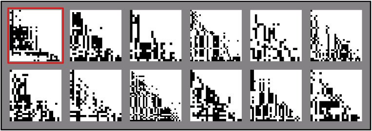
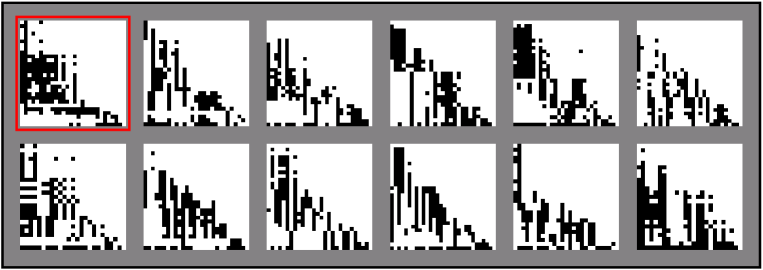
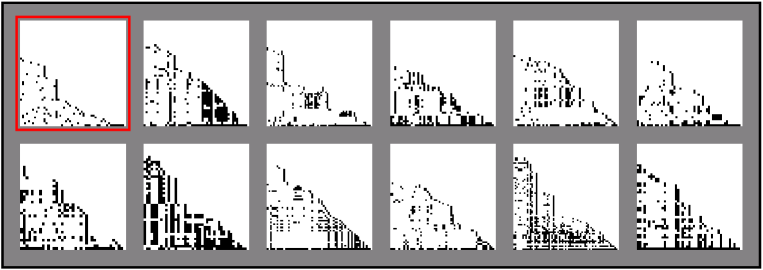
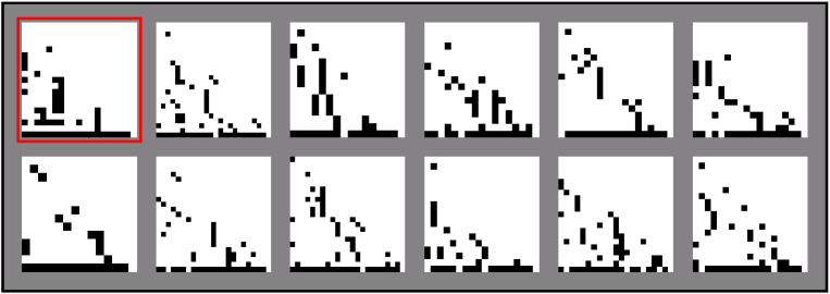
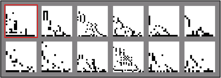
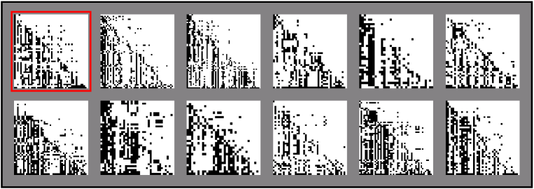
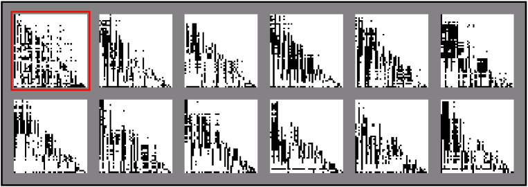
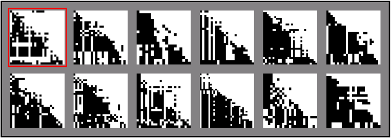
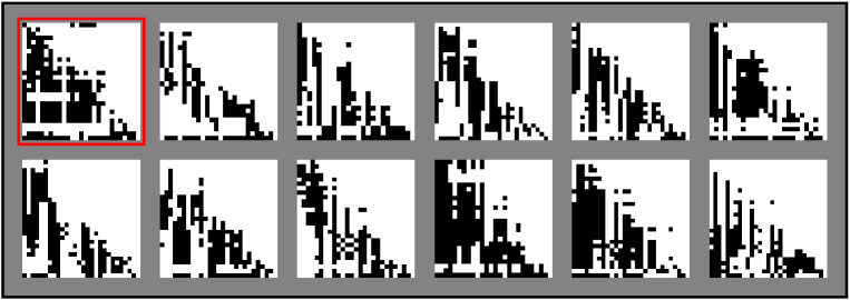
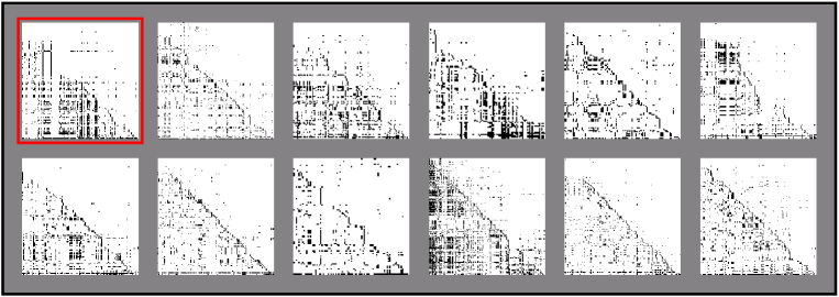
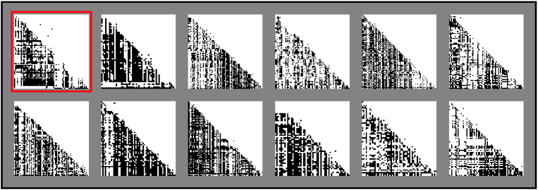
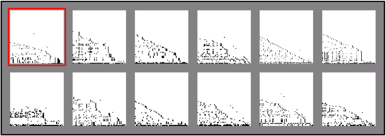
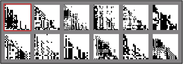
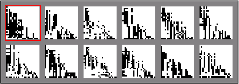
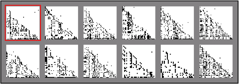
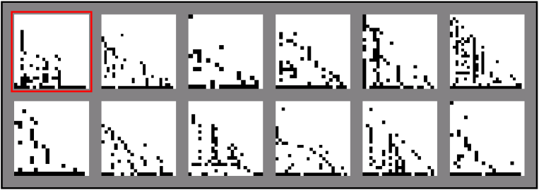
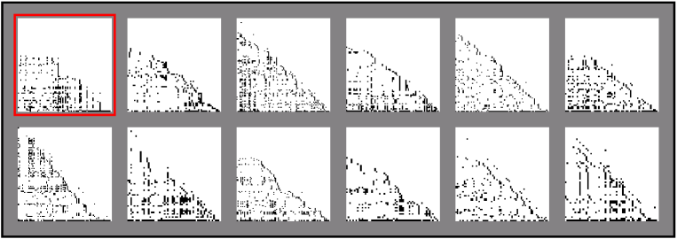
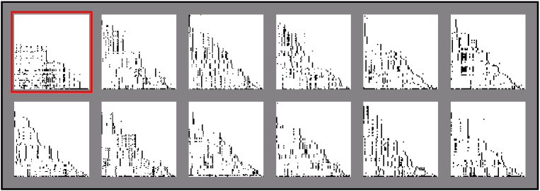
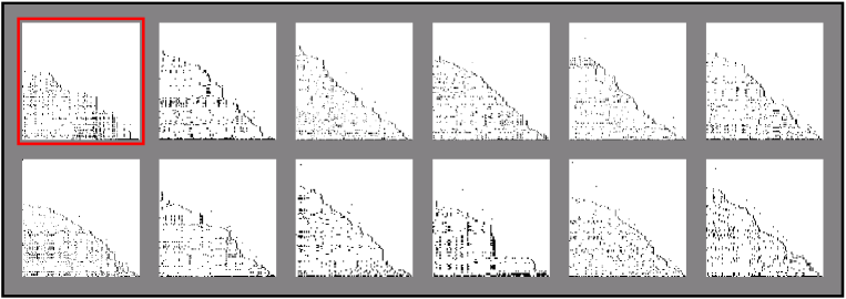
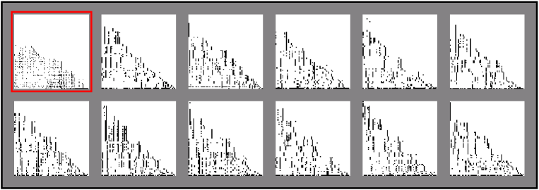
The connection matrix of the Caribbean Reef web (red box) is compared to the matrices of 11 random steady-state webs generated by the matching model (parameters as in Table 1). Each black pixel indicates that the species corresponding to its column eats the species corresponding to its row. Diagonal elements correspond to cannibalism. Pixel sizes vary due to varying webs sizes. For better comparison, data are displayed after standardization, a random permutation of all species, and a subsequent re-ordering such as to minimize entries in the upper triangle. Characteristic are, among others, the vertically stretched structures cattin04:_phylog reflecting the strong inheritance of consumer sets.
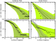
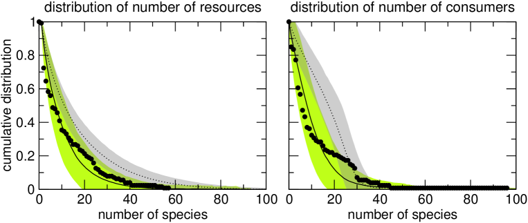
Cumulative distributions for the number of resources (upper panels) and consumers (lower panels) of species for the Caribbean Reef and Scotch Broom webs after data standardization. Points denote empirical data, solid and dotted lines model averages for matching and niche model, respectively. -ranges are indicated in green (matching model) and grey (niche model), olive at overlaps. Model parameters as in Table 1.
![[Uncaptioned image]](/html/q-bio/0508002/assets/x4.png)
Figure 1
![[Uncaptioned image]](/html/q-bio/0508002/assets/x5.png)
Figure 2
![[Uncaptioned image]](/html/q-bio/0508002/assets/x6.png)
Figure 3
Supplementary Information
Supplementary Methods
Supplementary Methods.1 Food-Web Data
The food-web data base used in this work was provided by N. D. Martinez and his team. The following are references the original sources: Benguela Current yodzis98:_local_benguel_interactions, Bridge Brook Lake havens92:_scale_webs, British Grassland martinez99:_effec_sampl_effor_charac_food_web_struc, Canton Creek townsend98:_distur, Caribbean Reef opitz96:_troph_carib, Chesapeake Bay baird89:_chesap_bay, Coachella Valley polis91:_compl_des_web, El Verde Rainforest waide96:_food_web_tropic_rainf, Little Rock Lake martinez91:_artif_attr, Northeast US Shelf link02:_does_web_theory, Scotch Broom memmott00:_predat_size_web, Skipwith Pond warren89:_spatial_freshw_web, St. Marks Seegrass christian99:_winter_seegrass, St. Martin Island goldwasser93:_const_carib_web, Stony Stream townsend98:_distur, Ythan Estuary 1 hall91:_food_rich_web, Ythan Estuary 2 huxham96:_do_parasites.
Supplementary Methods.2 Statistical Analysis
Supplementary Methods.2.1 Data standardization
Both empirical and model data were evaluated/compared after applying a data standardization procedure to the raw data. The procedure consists of three steps:
-
1.
Deleting disconnected species and small, disconnected sub-webs. Graph theory predicts that there will be only a single large connected component. We keep only this large component.
-
2.
Lumping of all species at the lowest trophic level into a single “trophic species”. We do this, because in some data sets the lowest trophic level is already strongly lumped. For example, the Chesapeake Bay web contains a species “phytoplankton”, and Coachella Valley “plants/plant products”. On the other hand, food webs such as Little Rock Lake resolves the phytoplankton at the genus level. Lumping the lowest level improves data intercomparability.
-
3.
The usual lumping of trophically equivalent species into single “trophic species” cohen90:_commun_food_webs_AND_THEREIN.
For some data sets with a simple structure, this procedure leads to a considerable reduction of the web size (e.g., Bridge Brook Lake shrinking from 74 species to 15). But generally this is not the case.
Supplementary Methods.2.2 Food-Web Properties
Besides the number of species and the number of links expressed in terms of the directed connectance martinez91:_artif_attr , the following 12 food-webs properties were used to characterize and compare empirical and model webs: the clustering coefficient camacho02:_robus_patter_food_web_struc; dorogovtsev02:_evolut_networ (Clust in Supplementary Figure 1); the fractions of cannibalistic species williams00:_simpl (Cannib) and species without consumers cohen90:_commun_food_webs_AND_THEREIN (T, top predators); the relative standard deviation in the number of resource species schoener89:_food_webs (GenSD, generality s.d.) and consumers schoener89:_food_webs (VulSD, vulnerability s.d.); the web average of the maximum of a species’ Jaccard similarity jaccard08:_nouvel_florale with any other species williams00:_simpl (MxSim); the fraction of triples of species with two or more resources, which have sets of resources that cannot be ordered to be all contiguous on a line cattin04:_phylog (Ddiet); the average cohen90:_commun_food_webs_AND_THEREIN (aChnLg), standard deviation martinez91:_artif_attr (aChnSD), and average per-species standard deviation goldwasser93:_const_carib_web (aOmniv, omnivory) of the length of food chains, as well as the of their total number martinez91:_artif_attr (aChnNo), with the prefix a indicating that these quantities were computed using the fast, “deterministic” Berger-Shor approximation berger90:_approx_subgraph of the maximum acyclic subgraph (MAS) of the food web. The number of non-cannibal trophic links not included in the MAS was measured as aLoop. When the output MAS of the Berger-Shor algorithm was not uniquely defined, the average over all possible outputs was used.
All food-web properties were calculated after data standardization as described above.
Supplementary Methods.2.3 Goodness-of-fit statistics
Mean and covariance matrix of the food-web properties described above, including but not , were computed for the model steady state and projected rossberg05:_web to fixed at the empirical value. The corresponding log-likelihood and the of the empirical values were computed thereof assuming Gaussian distributions. See Ref. rossberg05:_web for details.
Supplementary Methods.2.4 Parameter Fitting
The fitting parameters listed in Table 1 (except ) were chosen such as to maximize the log-likelihood computed as described above (maximum likelihood estimates). Given the other parameters, was always adjusted such as to make the model expectation value of , determined from Monte Carlo simulations, match the empirical value. The Akaike Information Criterion follows directly from the log-likelihood of the best-fitting parameter set.
In order to compute a comparable Akaike Information Criterion for the niche model, some modification of the original prescription for this model williams00:_simpl were required:
-
•
We applied the data standardization (Supplementary Methods.2.1) to both model and empirical data,
-
•
determined the niche-model parameter williams00:_simpl , which controls the connectance, by a maximum-likelihood estimate as above, and
-
•
determined the number of species of model webs before data standardization such as to match the expected number of species after data standardization with the empirical data, just as described above for the parameter of the matching model.
References
Supplementary Discussion
Supplementary Discussion.1 Derivation of Link Dynamics for Large
Here we explain why the network dynamics of the matching model becomes independent of for large , if is properly adjusted as increases. First, consider a single trophic link from a (potential) consumer to a (potential) resource. Denote the foraging traits of the former by , the vulnerability traits of the latter by , where and .
Supplementary Discussion.1.1 Linking Probability
Consider the steady-state distribution of the link strength defined by
| (1) |
Since the and are equally, independently distributed, follows a binomial distribution with mean and standard deviation . The probability for a link to exceed the threshold is
| (2) |
The distribution of converges to a standard normal distribution of large . The linking probability converges to a fixed value if is adjusted such that converges to a fixed value .
Supplementary Discussion.1.2 Mutation as an Integrated Ornstein-Uhlenbeck Process
In the following we argue that the dynamics of between speciations can be characterized as an integrated Ornstein-Uhlenbeck process if is large. First, consider only a single link, as above. When the resource speciates, its vulnerability traits are inherited by the descendant species, but with probability they flip from to . If this single step can be divided into a series of small steps, where a property is flipped in each step with a small probability and otherwise left unchanged. Taking the possibility that properties are flipped repeatedly into account, one finds that the small steps are equivalent to the speciation step if
| (3) |
or
| (4) |
For sufficiently large one has . Then at most one trait is flipped in each step, and the change in is of order . As increases, it becomes arbitrarily small.
Denote the value of after the -th step by . At each step, if is known, the probability distribution of depends only on and . If , for example, one has with probability , with probability , and otherwise . Thus the dynamics of —and of —from step to step are Markov processes.
These three properties of the step-by-step dynamics of in the limit of large and
-
1.
normal distribution in the steady state
-
2.
Markov property
-
3.
arbitrarily small changes from step to step
identify the dynamics as an Ornstein-Uhlenbeck process gardiner90:_handb_stoch_method
| (5) |
where is a Wiener process gardiner90:_handb_stoch_method and . In particular, one finds
| (6) |
The value of for a link from a speciating resource to its consumer is given by the integral of Eq. (5) over a -interval of unit-length, starting with the value of for the ancestor. This implies that of the correlation of between direct relatives is and between relatives of -th degree . The corresponding results for a speciating consumer are obtained by replacing in Eq. (6) by .
For the inheritance of several links to unrelated (hence uncorrelated) consumers, Eq. (5) holds for each link, and the Wiener processes are uncorrelated. For links to unrelated resources correspondingly. For links to related species the Wiener processes are correlated. From invariance considerations regarding the temporal ordering of evolutionary events in local networks one finds that for relatives of -th degree this correlation is for species-as-consumers and for species-as-resources. The correlations between links to related species from a newly invading species also follow this pattern. This provides a full characterization of the link dynamics for large independent of .
Supplementary Discussion.2 Relation to Previous Analytic Results
In order to make the analytic characterizations of the degree distributions and other food-web properties obtained for an earlier model variant rossberg05:_spec accessible for the matching model, we derive an approximate description of the link dynamics that refers directly to the inheritance of connectivity between species, i.e., of the information if a link is present or not, rather than the inheritance of traits determining links.
Mathematically, this corresponds to a Markov approximation for the dynamics of the connectivity in the following form: If resource B speciates to C, its connectivity information to a consumer A is lost with a probability (independent of the previous history) and otherwise copied from B to C. When the information is lost, a link from C to A is established at random with probability .
The breaking probability can be obtained by equating the probabilities A eats C given that A eats C’s ancestor B for the exact description (in terms of and ) and the Markov approximation. This gives
| (7) |
with defined by Eq. (2). The corresponding expression for is obtained by replacing in Eq. (7) by . Results of Ref. rossberg05:_spec can be applied to the matching model with the replacement of the parameter in Ref. rossberg05:_spec by .
Most analytic results of Ref. rossberg05:_spec rely on the unrealistic assumption of consumers evolving much slower than their resources. This assumption is used to argue for
-
1.
fully developed correlations of connectivity from one consumer to related resources and
-
2.
absence of correlations for connectivity from one resource to related consumers.
Effects 1 and 2 are then used to simplify calculations. In the matching model 1 and 2 can be obtained without assuming large differences in speciation rates: Effect 1 is obtained because statistical correlations in connectivity to related resources in the matching model depend only on the correlations between the traits of the resources, and not on the evolutionary history of the consumer (see also Supplementary Discussion.1). The correlations are large if is small and, as a result, is small. Effect 2 is obtained when is close to (foraging traits are randomized in speciations), which implies that is close to .
Results of Ref. rossberg05:_spec that contribute to a better understanding of the matching model include the derivation of the conditions under which the degree distributions become those of the niche model, and the explanation why model webs, just as empirical data cohen90:_commun_food_webs_AND_THEREIN, exhibit a larger-than-random degree of “intervality”. The average number of resource “families” (or “clades”) of a consumer in the matching model can also be estimated, and turns out to be small: The largest value (3.7) is obtained for the top predator of Ythan Estuary 2. For most other webs this number is below two.
References
Supplementary Movie Legend
(The movie can be found at http://ag.rossberg.net/matching.mpg or http://www.envcomplex.ynu.ac.jp/matching.mpg.)
This 1 minute movie (MPEG, 7MB) illustrates the dynamics of the matching model. The movie shows the evolution of the connection matrix of food webs in the model steady state at parameters corresponding to Little Rock Lake (Table 1). Each black pixel indicates that the species corresponding to its column eats the species corresponding to its row. Diagonal elements correspond to cannibalism. To ensure temporal continuity, the raw data—prior to data standardization—are show. Thus, these matrices are not directly comparable to the matrices displayed in Figure 2 and Supplementary Figures 2-18. Species are sorted by decreasing size parameter from top to bottom and left to right. The movie shows one evolutionary event (speciation, extinction, invasion) per frame at 25 frames per second.
Supplementary Figure Legends
Supplementary Figure Legends.1 Results for Food-Web Properties
In Supplementary Figure 1 the best fitting results for the matching model (red starts) and for the niche model (blue boxes) are compared to the empirical data (horizontal lines). Vertical lines correspond to one model standard deviation. Because the properties are computed conditional to fixed , the value of always fits exactly. Note that the graph does not contain the full information about the covariance matrices that entered the and likelihood calculations, and therefore indicates the goodness of fit only semiquantitatively.
Supplementary Figure Legends.2 More connection matrixes and degree distributions
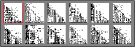
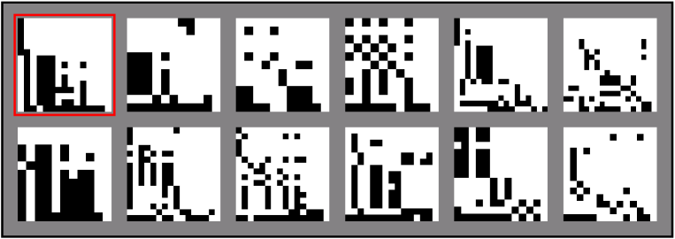
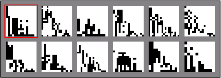
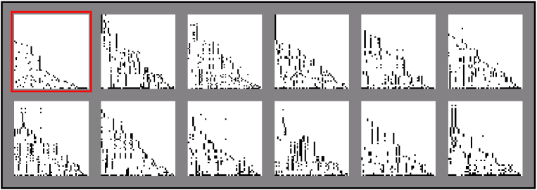
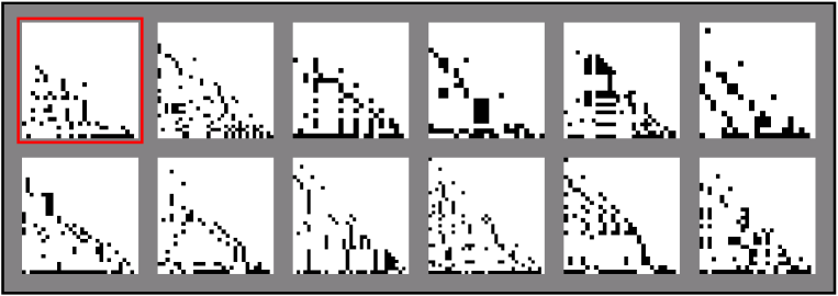
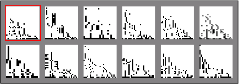
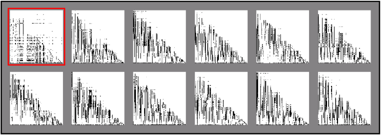
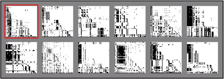
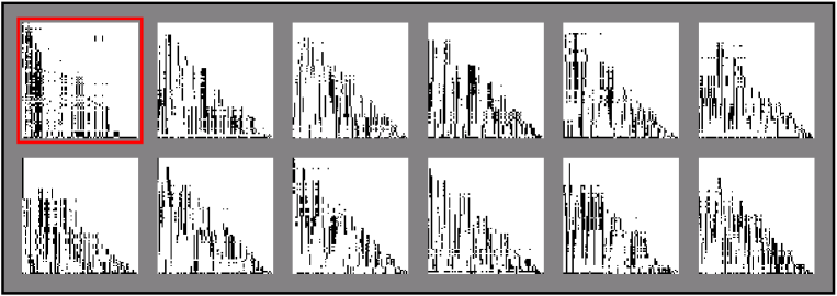
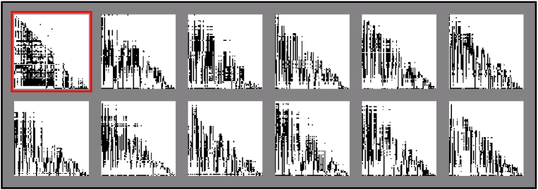
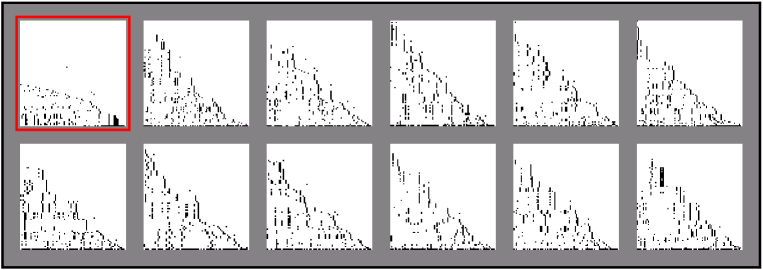
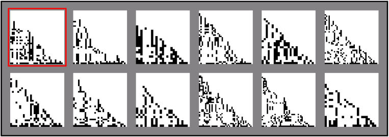
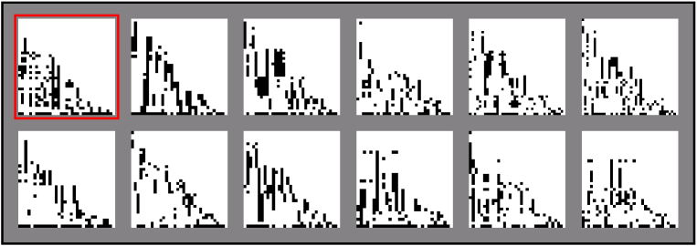
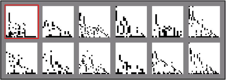
Supplementary Figures 2 to 18 present the results corresponding to Figures 2 and 3 (main text) for all food webs and the two models considered. In each figure, the first panel shows the connection matrix of the empirical food web in a red box compared to the first 11 random samples obtained from a simulation of the matching model. As in Figure 2, each black pixel indicates that the species corresponding to its column eats the species corresponding to its row. Diagonal elements correspond to cannibalism. Pixel sizes vary due to varying webs sizes. Data are displayed after standardization, a random permutation of all species, and a subsequent re-ordering such as to minimize entries in the upper triangle. The second panel in each figure displays the corresponding data for the niche model.
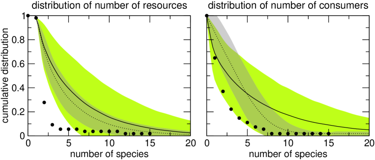
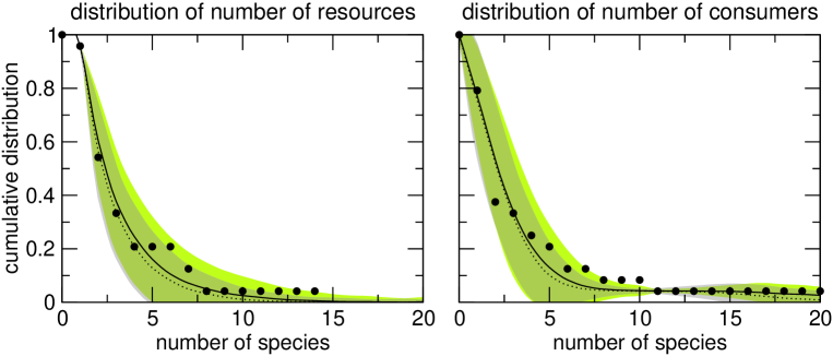
The two bottom panels compare model and empirical degree distributions (model parameters as in Table 1). As in Figure 3, points denote empirical data, and solid and dotted lines model averages for matching and niche model, respectively; -ranges are indicated in green (matching model) and grey (niche model), olive at overlaps. All model distributions were calculated conditional to fixed at the empirical value.
Since, for the purpose of data standardization, the lowest trophic level is lumped to a single trophic species, there is always exactly one “species” that does not consume others. As a result, the second point in the cumulative distribution of the number of resources is always fixed at . Because the consumers of this lumped species are the consumers of all species that were lumped into it, the number of consumers of the lumped species is comparatively large, which leads to a leveling-off at the tails of consumer distributions as compared to the distributions for the raw data shown in Ref. stouffer05:_quant_patterns_webs.
The informations provided by the connection matrices and the degree distributions are complementary. While the degree distributions give integral information regarding the whole web, the connection matrices give an impression of the correlations present between individual species as well as the fluctuations in the steady state.
References
Supplementary Figures
Matching model:
Niche model:
Matching model:
Niche model:
Matching model:
Niche model:
Matching model:
Niche model:
Matching model:
Niche model:
Matching model:
Niche model:
Matching model:
Niche model:
Matching model:
Niche model:
Matching model:
Niche model:
Matching model:
Niche model:
Matching model:
Niche model:
Matching model:
Niche model:
Matching model:
Niche model:
Matching model:
Niche model:
Matching model:
Niche model:
Matching model:
Niche model:
Matching model:
Niche model:
never {never}