Error thresholds in a mutation–selection model with Hopfield-type fitness

Abstract

A deterministic mutation–selection model in the sequence space approach is investigated. Genotypes are identified with two-letter sequences. Mutation is modelled as a Markov process, fitness functions are of Hopfield type, where the fitness of a sequence is determined by the Hamming distances to a number of predefined patterns. Using a maximum principle for the population mean fitness in equilibrium, the error threshold phenomenon is studied for quadratic Hopfield-type fitness functions with small numbers of patterns. Different from previous investigations of the Hopfield model, the system shows error threshold behaviour not for all fitness functions, but only for certain parameter values.

1 Introduction

Population genetics is concerned with the investigation of the genetic structure of populations, which is influenced by evolutionary factors such as mutation, selection, recombination, migration and genetic drift. For excellent reviews of the theoretical aspects of this field, see Baake and Gabriel (2000); Crow and Kimura (1970); Ewens (2004).

In this paper, the antagonistic interplay of mutation and selection shall be investigated, with mutation generating the genetic variation upon which selection can act. Pure mutation–selection models exclude genetic drift and are therefore deterministic models, and accurate only in the limit of an infinite population size (for a review, see Bürger, 2000). A further simplification taken here is to consider only haploid populations, where the genetic material exists in one copy only in each cell. However, the equations used here to describe evolution apply as well to diploid populations without dominance.

For the modelling of the types considered, the sequence space approach is used, which has first been used by Eigen (1971) to model the structure of the DNA, where individuals are taken to be sequences. Here, the sequences shall be written in a two-letter alphabet, thus simplifying the full four-letter structure of DNA sequences. In this approach, the modelling is based on the microscopic level, at which the mutations occur, hence the mutation process is fairly straightforward to model. However, the modelling of selection is a more challenging task, as selection acts on the phenotype, and the mapping from genotype to phenotype is by no means simple. To this end, the concept of the fitness landscape (Kauffman and Levin, 1987) is introduced as a function on the sequence space, assigning to each possible genotype a fitness value which determines the reproduction rate. Apart from the problem that a realistic fitness landscape would have to be highly complex (too complex for a mathematical treatment), there is also very limited information available concerning the nature of realistic fitness functions. Therefore, the modelling of fitness is bound by feasibility, trying to mimic general features that are thought to be essential for realistic fitness landscapes such as the degree of ruggedness.

A very common type of fitness functions is the class of permutation-invariant fitness functions, where the fitness of a sequence is determined by the number of mutations it carries compared to the wild-type, but not on the locations of the mutations within the sequence. Although this model describes the accumulation of small mutational effects surprisingly well, it is a simplistic model that lacks a certain degree of ruggedness that is thought to be an important feature of realistic fitness landscapes (Baake and Gabriel, 2000).

In this paper, Hopfield-type fitness functions (Hopfield, 1982) are treated as a more complex model. Here, the fitness of a sequence is not only determined by the number of mutations compared to one reference sequence, but to a number of predefined sequences, the patterns. This yields a class of fitness landscapes that contain a higher degree of ruggedness, which can be tuned by the number of patterns chosen. While this can still be treated with the methods used here, it is a definite improvement on the restriction of permutation-invariant fitness functions.

Particular interest is taken in the phenomenon of mutation driven error thresholds, where the population in equilibrium changes from viable to non-viable within a narrow regime of mutation rates. In this paper, a few examples of Hopfield-type fitness functions are investigated with respect to the error threshold phenomenon.

Section 2 introduces the basic mutation–selection model with its main observables. In section 3, the model is applied to the sequence space approach, formulating the mutation and fitness models explicitly. Sections 4 and 5 present the method, which relies on a lumping of the large number of sequences into classes on which a coarser mutation–selection process is formulated. This lumping is necessary to formulate a simple maximum principle to determine the population mean fitness in equilibrium. In section 6, this maximum principle is used to investigate some examples of Hopfield-type fitness functions with respect to the error threshold phenomenon.

2 The mutation–selection model

The model used here (as detailed below) is a pure mutation–selection model in a time-continuous formulation as used by Hermisson et al. (2002) and Garske and Grimm (2004b, a), for instance.

Population.

The evolution of a population where the only evolutionary forces are mutation and selection is considered, thus excluding other factors such as drift or recombination for instance. Individuals in the population shall be assigned a type $i$ from the finite type space $\mathfrak{S}$. The population at any time $t$ is described by the population distribution $\boldsymbol{p}(t)$, a vector of dimension $|\mathfrak{S}|$, the cardinality of the type space. An entry $p_{i}(t)$ gives the fraction of individuals in the population that are of type $i$. Thus the population is normalised such that $\sum_{i}p_{i}(t)=1$.

Evolutionary processes.

The evolutionary processes that occur are birth, death and mutation events. Birth and death events occur with rates $b_{i}$ and $d_{i}$ that depend on the type $i$ of the individual in question, and taken together, they give the effective reproductive rate, or fitness as $r_{i}=b_{i}-d_{i}$. Mutation from type $i$ to type $j$ depends on both initial and final type and happens with rate $m_{ji}$. These rates are conveniently collected in square matrices $\mathcal{R}$ and $\mathcal{M}$ of dimension $|\mathfrak{S}|$, where the reproduction or fitness matrix $\mathcal{R}$ with entries $r_{i}$ is diagonal. The off-diagonal entries of the mutation matrix $\mathcal{M}$ are given by the mutation rates $m_{ji}$, and as mutation does not change the number of individuals, the diagonal entries of $\mathcal{M}$ are chosen such that $\mathcal{M}_{ii}=-\sum_{j\neq i}\mathcal{M}_{ji}$, which makes $\mathcal{M}$ a Markov generator. The time evolution operator $\mathcal{H}$ is given by the sum of reproduction and mutation matrix, $\mathcal{H}=\mathcal{R}+\mathcal{M}$.

Deterministic evolution equation.

In the deterministic limit of an infinite population size, the evolution of the population is governed by the evolution equation

$$\boldsymbol{\dot{p}}(t)=\left[\mathcal{H}-\bar{r}(t)\boldsymbol{1}\right]\boldsymbol{p}(t)\;,$$ (1)

where $\bar{r}(t)=\sum_{i}r_{i}p_{i}(t)$ is the population mean fitness. The term with $\bar{r}$ is needed to preserve the normalisation of the population. Note that this term makes the evolution equation (1) nonlinear.

Equilibrium.

The main interest focuses on the equilibrium, i.e., the behaviour if $\boldsymbol{\dot{p}}=0$, which is attained for $t\rightarrow\infty$. All equilibrium quantities shall be denoted by omitting the argument $t$, for instance the equilibrium population distribution is $\boldsymbol{p}$. In equilibrium, the evolution equation (1) becomes an eigenvalue equation for $\mathcal{H}$, with leading eigenvalue $\bar{r}$ and corresponding eigenvector $\boldsymbol{p}$. If $\mathcal{M}$ is irreducible, as shall be assumed throughout, Perron-Frobenius theory (see, for instance, Karlin, 1966, appendix) applies, which guarantees that the leading eigenvalue $\bar{r}$ of $\mathcal{H}$ is non-degenerate and the corresponding right eigenvector $\boldsymbol{p}$ is strictly positive, which implies that it can be normalised as a probability distribution.

Ancestral distribution.

Similarly to the population distribution $\boldsymbol{p}$, there is also another important distribution in this model, namely the ancestral distribution $\boldsymbol{a}(\tau,t)$. Consider the population at time $t+\tau$, but count each individual not as its current type, but as the type its ancestor had at time $t$. Thus an entry of the ancestral distribution $a_{i}(\tau,t)$ determines the fraction of the population at $t+\tau$ whose ancestor at time $t$ was of type $i$. In the limit $\tau,t\rightarrow\infty$, this also approaches an equilibrium distribution $\boldsymbol{a}$. As shown by Hermisson et al. (2002), the equilibrium ancestral distribution can be obtained as a product of the left and right PF (Perron-Frobenius) eigenvectors $\boldsymbol{z}$ and $\boldsymbol{p}$ of the time-evolution operator $\mathcal{H}$ as $a_{i}=z_{i}p_{i}$, where $\boldsymbol{z}$ is normalised such that $\sum_{i}a_{i}=1$.

Population and ancestral means.

Any function on the type space given, say, by $f=(f_{i})_{i\in\mathfrak{S}}$ can be averaged with respect to the population or the ancestral distribution distribution. The population mean of $f$ is given by

$$\bar{f}(t)=\sum_{i}f_{i}p_{i}(t)\;,$$ (2)

whereas the ancestral mean is

$$\hat{f}(\tau,t)=\sum_{i}f_{i}a_{i}(\tau,t)\;.$$ (3)

Note that the time-dependence of the means only comes from the distribution, whereas the function $f$ is considered constant in time. In equilibrium, time dependence is again omitted such that the equilibrium population and ancestral means are denoted $\bar{f}$ and $\hat{f}$, respectively. An important example of the population mean is the population mean fitness $\bar{r}(t)$ from equation (1).

3 Sequences as types

In the previous section, the types are a rather abstract concept. In order to formulate the particular mutation and fitness models, they shall now be specified as sequences, mimicking the structure of the DNA (cf. Eigen, 1971). For simplicity, only two-state sequences are considered, i.e., sequences that have at each site one out of two possible entries. However, the method used here can immediately be generalised to a more realistic four-state model (see Garske, 2005).

The types therefore are associated with sequences $\boldsymbol{\sigma}=\sigma_{1}\sigma_{2}\ldots\sigma_{N}$ of fixed length $N$, written in the alphabet $\mathcal{A}=\{0,1\}$, thus $\sigma_{\alpha}\in\mathcal{A}$ for $\alpha=1,\ldots,N$. This means that there are $2^{N}$ different sequences, and thus the type space (or sequence space) $\mathfrak{S}$ has cardinality $|\mathfrak{S}|=2^{N}$.

3.1 Mutation model

A simple mutation model that neglects any processes changing the length of the sequence, such as deletions or insertions, is used. Mutations are modelled as point processes, where an arbitrary site $\sigma_{\alpha}$ is switched with rate $\mu$, such that the mutation rate between sequences that differ only in one particular site is given by $\mu/N$. Sequences that differ in more than one site cannot mutate into one another within a single mutational step. This is known as the single step mutation model, introduced by Ohta and Kimura (1973).

The mutation model defines a neighbourhood in the sequence space (Reidys and Stadler, 2002). A convenient measure for the distance between sequences is the Hamming distance $d_{H}(\boldsymbol{\sigma},\boldsymbol{\sigma^{\prime}})$, which counts the number of sites at which the sequences $\boldsymbol{\sigma}$ and $\boldsymbol{\sigma^{\prime}}$ differ (Hamming, 1950; van Lint, 1982). With this, the mutation matrix is explicitly given as

$$\mathcal{M}_{\boldsymbol{\sigma\sigma^{\prime}}}=\begin{cases}\mu/N&\text{if $d_{H}(\boldsymbol{\sigma},\boldsymbol{\sigma^{\prime}})=1$\,,}\\ 0&\text{if $d_{H}(\boldsymbol{\sigma},\boldsymbol{\sigma^{\prime}})>1$\,,}\\ -\mu&\text{if $\boldsymbol{\sigma}=\boldsymbol{\sigma^{\prime}}$\,.}\end{cases}$$ (4)

The diagonal entry is chosen such that $\mathcal{M}$ fulfils the Markov condition $\sum_{j}\mathcal{M}_{ji}=0$.

3.2 Fitness functions

A rather simple, though commonly used type of fitness function is the permutation-invariant fitness. There, the fitness of a sequence depends only on the number of mutations it has compared to a reference type, not on their position along the sequence. Thus fitness is a function of the Hamming distance to the reference sequence, which is usually chosen as the wild-type. The Hamming distance to the wild-type is also called the mutational distance $d$.

A non-permutation-invariant fitness that contains some ruggedness, but is simple enough to be dealt with in this framework, is the Hopfield-type fitness, a special type of spin-glass model, which has been introduced by Hopfield (1982) as a model for neural networks. Instead of comparing a sequence only to the wild-type, as it is done for the permutation-invariant fitness, the Hopfield-type fitness of a sequence is determined by its Hamming distances to $p+1$ reference sequences, the patterns $\boldsymbol{\xi}^{q}$, $q=0,\ldots,p$. The Hopfield-type fitness shall be defined in terms of the specific distances $w^{q}$, which are the Hamming distances with respect to the patterns,

$$w^{q}=d_{H}(\boldsymbol{\xi}^{q},\boldsymbol{\sigma})\,,$$ (5)

and thus the fitness is given as

$$r_{\boldsymbol{\sigma}}=r_{\boldsymbol{\sigma}}((w^{q})_{q=0,\ldots,p})\,.$$ (6)

Note that in the case of a single pattern ($p=0$), this yields again a permutation-invariant fitness.

4 Lumping for the Hopfield-type fitness

4.1 The general lumping procedure

One problem of the sequence space approach is the large number of types, which grows exponentially with the sequence length $N$, $|\mathfrak{S}|=2^{N}$. The time-evolution operator $\mathcal{H}$ is a matrix of size $|\mathfrak{S}|\times|\mathfrak{S}|$, and in this set-up one is interested in its leading eigenvalue $\bar{r}$ and the corresponding right and left eigenvectors $\boldsymbol{p}$ and $\boldsymbol{z}$.

The relevant sequence length depends on the particular application one has in mind, but it is typically rather long. If one aims to model the whole genome of a virus or a bacterium, $N$ has to be in the region of $N\approx 10^{6}$, but even a single gene has of the order of $N\approx 10^{3}$ base pairs. These values lead to matrices of a size that makes the eigenvalues and eigenvectors inaccessible.

For some types of fitness functions, this problem can be reduced by lumping together types into classes of types, and considering the new process on a reduced sequence space, which contains the classes rather than the individual types. Under certain circumstances, mutation is described as a Markov process in the emerging lumped process as well, such that this process is accessible to Markov process methods, and the framework developed in section 2 can directly be applied to the lumped system.

The lumping of the mutation process is a standard procedure in the theory of Markov chains (Kemeny and Snell, 1960, chapter 6), see also Baake et al. (2005) for an application to mutation–selection models. This lumping leads to a meaningful mutation–selection model on the reduced type space, if all sequences lumped together into one class have the same fitness.

It is possible to lump the Markov chain given by the mutation matrix $\mathcal{M}$ with state space $\mathfrak{S}$ with respect to a particular partition $\mathfrak{S}=\dot{\bigcup}_{k=0}^{r}\mathfrak{S}_{k}$, if and only if for each pair $\mathfrak{S}_{k},\mathfrak{S}_{\ell}$ the cumulative mutation rates

$$u_{\mathfrak{S}_{\ell},i}:=\sum_{j\in\mathfrak{S}_{\ell}}\mathcal{M}_{ji}$$ (7)

from type $i\in\mathfrak{S}_{k}$ into $\mathfrak{S}_{\ell}$, are identical for all $i\in\mathfrak{S}_{k}$, cf. the example shown in figure 1.

Figure 1: Visualisation of the compatibility with lumping: Consider two classes $\mathfrak{S}_{k}$ and $\mathfrak{S}_{\ell}$. The mutation rates from the types in $\mathfrak{S}_{k}$ to the types in $\mathfrak{S}_{\ell}$ (given next to the arrows) are compatible with a lumping with respect to $\mathfrak{S}_{k}$ and $\mathfrak{S}_{\ell}$, because the sum of the mutation rates from type $i_{1}$ to all types in $\mathfrak{S}_{\ell}$ is given by $u_{\mathfrak{S}_{\ell},{i_{1}}}=1+1+2=4$, which is identical with those from $i_{2}$, $u_{\mathfrak{S}_{\ell},{i_{2}}}=3+0+1=4$.

In this case, the lumped process, with $r+1$ states $\mathfrak{S}_{0},\ldots,\mathfrak{S}_{r}$ and mutation rates $u_{{\mathfrak{S}_{\ell}},{i}}$ for any $i\in\mathfrak{S}_{k}$, is again a Markov chain (Kemeny and Snell, 1960, theorem 6.3.2).

4.2 Defining the partial distances

Whereas in the case of a permutation-invariant fitness function, the lumping procedure is fairly simple, collecting all sequences with the same Hamming distance to the wild-type into classes, and considering cumulative mutation rates between these classes, the lumping for the Hopfield-type fitness is somewhat more complex. For a two-state model with Hopfield fitness, it has been performed for instance by Baake et al. (2005), and this shall be recollected in the remainder of this section.

First, the quantities with respect to which the lumping shall be performed must be defined. To this end, consider as an example the case of sequence length $N=12$ with three patterns ($p=2$), and let the patterns $\boldsymbol{\xi}^{q}$ be collected in a $(p+1)\times N$ matrix $\boldsymbol{\xi}$, such that the $q$th row of $\boldsymbol{\xi}$ is pattern $\boldsymbol{\xi}^{q}$. Without loss of generality, the pattern $\boldsymbol{\xi}^{0}$ can always be chosen as $\boldsymbol{\xi}^{0}=000\ldots 0$. Let the patterns in this example be given as

$$\boldsymbol{\xi}=\begin{pmatrix}\boldsymbol{\xi}^{0}\\ \boldsymbol{\xi}^{1}\\ \boldsymbol{\xi}^{2}\end{pmatrix}=\setcounter{MaxMatrixCols}{12}\begin{pmatrix}0&0&0&0&0&0&0&0&0&0&0&0\\ 1&0&1&1&0&1&0&1&1&1&0&0\\ 1&0&0&0&1&1&1&1&1&1&1&0\end{pmatrix}\,.$$ (8)

Note that there are only $2^{p}$ different types of sites (corresponding to the columns of $\boldsymbol{\xi}$). These are collected in a $(p+1)\times 2^{p}$ matrix $\boldsymbol{\rho}$, the columns of which correspond to the possible types of sites in the matrix of patterns $\boldsymbol{\xi}$. For the case $p=2$, this $3\times 4$ matrix is given as

$$\boldsymbol{\rho}=\begin{pmatrix}0&0&0&0\\ 0&0&1&1\\ 0&1&0&1\end{pmatrix}\,.$$ (9)

Using the column vectors $\boldsymbol{\rho}_{v}$ of the matrix $\boldsymbol{\rho}$, the patterns given in equation (8) can alternatively be expressed as

$$\boldsymbol{\xi}=\left(\boldsymbol{\rho}_{4},\boldsymbol{\rho}_{1},\boldsymbol{\rho}_{3},\boldsymbol{\rho}_{3},\boldsymbol{\rho}_{2},\boldsymbol{\rho}_{4},\boldsymbol{\rho}_{2},\boldsymbol{\rho}_{4},\boldsymbol{\rho}_{4},\boldsymbol{\rho}_{4},\boldsymbol{\rho}_{2},\boldsymbol{\rho}_{1}\right)\,,$$ (10)

classifying the sites into $2^{p}$ classes according to which of the column vectors $\boldsymbol{\rho}_{v}$ of $\boldsymbol{\rho}$ coincides with the column vector $\boldsymbol{\xi}_{\alpha}$ of the patterns $\boldsymbol{\xi}$ at site $\alpha$.

Let $\Lambda=\{1,\ldots,N\}$ be the index set of sites, with a partition into $2^{p}$ subsets $\Lambda_{v}$ induced by the patterns $\boldsymbol{\xi}$ such that

$$\Lambda=\dot{\bigcup}_{v=1}^{2^{p}}\Lambda_{v}\,,$$ (11)

with

$$\alpha\in\Lambda_{v}\quad\Longleftrightarrow\quad\boldsymbol{\xi}_{\alpha}=\boldsymbol{\rho}_{v}\,.$$ (12)

Patterns can be characterised by the number of sites $N_{v}=|\Lambda_{v}|$ in each subset. The example patterns (8) can therefore be described by

$$\Lambda_{1} =\{2,12\}\,, \Lambda_{2} =\{5,7,11\}\,, \Lambda_{3} =\{3,4\}\,, \Lambda_{4} =\{1,6,8,9,10\}\,,$$

$$N_{1} =2\,, N_{2} =3\,, N_{3} =2\,, N_{4} =5\,.$$ (13)

Considering only subsequences $\boldsymbol{\sigma}_{v}:=(\sigma_{\alpha})_{\alpha\in\Lambda_{v}}$, the partial distances $d_{v}$ of a sequence $\boldsymbol{\sigma}$ with respect to the pattern $\boldsymbol{\xi}^{0}$ are defined as the Hamming distance between $\boldsymbol{\sigma}$ and $\boldsymbol{\xi}^{0}$, restricted to the subsequence $\boldsymbol{\sigma}_{v}$. Therefore, they can be written as

$$d_{v}:=\sum_{\alpha\in\Lambda_{v}}\delta(1,\sigma_{\alpha})\quad\mbox{with}\quad 0\leq d_{v}\leq N_{v}\,,$$ (14)

such that the specific distance with respect to pattern $\boldsymbol{\xi}^{0}$ is given by $w^{0}=\sum_{v=1}^{2^{p}}d_{v}$.

Because the differences between each of the patterns $\boldsymbol{\xi}^{q}$ within the subsets $\Lambda_{v}$ of $\Lambda$ are known (and recorded in the matrix $\boldsymbol{\rho}$), it is sufficient to consider only the partial distances $d_{v}$ with respect to one pattern, here $\boldsymbol{\xi}^{0}$; the partial distances $d_{v}^{q}$ with respect to any other pattern can be expressed in terms of the $d_{v}$ as

$$d_{v}^{q}=\sum_{\alpha\in\Lambda_{v}}\delta(1-\rho_{v}^{q},\sigma_{\alpha})=\begin{cases}d_{v}&\text{if $\rho_{v}^{q}=0$,}\\ N_{v}-d_{v}&\text{if $\rho_{v}^{q}=1$,}\\ \end{cases}$$ (15)

using the matrix elements $\rho_{v}^{q}$ of $\boldsymbol{\rho}$.

The specific distance $w^{q}$ to any pattern $\boldsymbol{\xi}^{q}$ can be expressed as

$$w^{q}=\sum_{v=1}^{2^{p}}\sum_{\alpha\in\Lambda_{v}}\delta(1-\rho_{v}^{q},\sigma_{\alpha})=\sum_{v\in V_{0}^{q}}d_{v}+\sum_{v\in V_{1}^{q}}(N_{v}-d_{v})\,,$$ (16)

where the index set $V=\{1,\ldots,2^{p}\}$ of classes is partitioned into two subsets, $V=V_{0}^{q}\cup V_{1}^{q}$ with $V_{0}^{q}=\{v|\rho_{v}^{q}=0\}$ and $V_{1}^{q}=\{v|\rho_{v}^{q}=1\}$.

Hence, by specifying the $2^{p}$ partial distances $d_{v}$ with respect to pattern $\boldsymbol{\xi}^{0}$, the specific distances $w^{q}$ with respect to any pattern $\boldsymbol{\xi}^{q}$ are determined, which in turn determine the fitness. This implies that all sequences with the same partial distances $d_{v}$ have the same fitness. Thus the partial distances $d_{v}$ to pattern $\boldsymbol{\xi}^{0}$, collected in a mutational distance vector $\boldsymbol{d}=(d_{v})_{v=1\ldots 2^{p}}$, shall be the quantities that label the classes in the lumped system.

4.3 Lumping with respect to the partial distances

The relevant partition of the sequence space is given by $\mathfrak{S}=\dot{\bigcup}_{\boldsymbol{d}}\mathfrak{S}_{\boldsymbol{d}}$ with $\mathfrak{S}_{\boldsymbol{d}}=\{\boldsymbol{\sigma}|\boldsymbol{d}_{\boldsymbol{\sigma}}=\boldsymbol{d}\}$, and the reduced sequence space, or mutational distance space $\mathcal{S}$, contains the classes $\mathcal{S}=\{\boldsymbol{d}|0\leq d_{v}\leq N_{v},v=1\ldots 2^{p}\}$.

Considering again the subsequences $\boldsymbol{\sigma}_{v}$, there are $N_{v}+1$ possible different $d_{v}$ (as $d_{v}$ takes values from $0$ to $N_{v}$), and there are $\binom{N_{v}}{d_{v}}$ different subsequences $\boldsymbol{\sigma}_{v}$ for each $d_{v}$. Hence, considering all sites, there are

$$|\mathcal{S}|=\prod_{v=1}^{2^{p}}(N_{v}+1)$$ (17)

different $\boldsymbol{d}$, and

$$n_{\boldsymbol{d}}=\prod_{v=1}^{2^{p}}\binom{N_{v}}{d_{v}}$$ (18)

sequences $\boldsymbol{\sigma}$ that are mapped onto each $\boldsymbol{d}$. For the patterns $\boldsymbol{\xi}$ chosen as example (8), we have $|\mathcal{S}|=3\cdot 4\cdot 3\cdot 6=216$, while the full sequence space has dimension $|\mathfrak{S}|=2^{12}=4096$.

In the single step mutation model, the only neighbours of a sequence $\boldsymbol{\sigma}$ with distance vector $\boldsymbol{d}$ lie in the classes $\boldsymbol{d}\pm\boldsymbol{e}_{v}$, where the $\boldsymbol{e}_{v}=(\delta_{vw})_{w=1\ldots 2^{p}}$ are the unit vectors of mutation. Thus the only non-zero cumulative mutation rates are

$$u^{\pm v}_{\boldsymbol{d}}:=u_{\boldsymbol{d}\pm\boldsymbol{e}_{v},\boldsymbol{\sigma}}=\sum_{\boldsymbol{\sigma}^{\prime}\in\mathfrak{S}_{\boldsymbol{d}\pm\boldsymbol{e}_{v}}}\mathcal{M}_{\boldsymbol{\sigma}^{\prime}\boldsymbol{\sigma}}\,.$$ (19)

As a sequence with $\boldsymbol{d}$ has $(N_{v}-d_{v})$ $0$-sites and $d_{v}$ $1$-sites in $\Lambda_{v}$, and the single-site mutation rates are $\mu/N$ for all sites, the cumulative mutation rates are given by

$$u^{+v}_{\boldsymbol{d}} =\mu\,(N_{v}-d_{v})/N \boldsymbol{d}\rightarrow\boldsymbol{d}+\boldsymbol{e}_{v}$$ for and

$$u^{-v}_{\boldsymbol{d}} =\mu\,d_{v}/N \boldsymbol{d}\rightarrow\boldsymbol{d}-\boldsymbol{e}_{v}$$ for , (20)

irrespective of the particular order within the subsequences $\boldsymbol{\sigma}_{v}$. Therefore the cumulative mutation rates $u^{\pm v}_{\boldsymbol{d}}$ are the same for all sequences $\boldsymbol{\sigma}$ with the same $\boldsymbol{d}$, which is the condition for lumping. The mutation–selection model with Hopfield-type fitness is indeed “lumpable” with respect to the partition induced by the distance vectors $\boldsymbol{d}$.

The mutation–selection process on the mutational distance space $\mathcal{S}$ is described by the lumped time-evolution operator $\boldsymbol{H}=\boldsymbol{R}+\boldsymbol{M}$ with lumped reproduction and mutation matrices $\boldsymbol{R}$ and $\boldsymbol{M}$ of dimension $|\mathcal{S}|\times|\mathcal{S}|$. Whereas the lumped reproduction matrix $\boldsymbol{R}$ is still diagonal and contains the same entries as $\mathcal{R}$, i.e. $\boldsymbol{R}_{\boldsymbol{d}_{\boldsymbol{\sigma}}}=\mathcal{R}_{\boldsymbol{\sigma}}$, the off-diagonal entries of the lumped mutation matrix $\boldsymbol{M}$ are given by the cumulative mutation rates with unchanged diagonal entries compared to $\mathcal{M}$, which still fulfil the Markov property $\boldsymbol{M}_{\boldsymbol{dd}}=-\sum_{\boldsymbol{d}^{\prime}\neq\boldsymbol{d}}M_{\boldsymbol{d}^{\prime}\boldsymbol{d}}$, and thus

$$M_{\boldsymbol{d}^{\prime}\boldsymbol{d}}=\begin{cases}u^{+v}_{\boldsymbol{d}}&\text{if $\boldsymbol{d}^{\prime}=\boldsymbol{d}+\boldsymbol{e}_{v}$,}\\ u^{-v}_{\boldsymbol{d}}&\text{if $\boldsymbol{d}^{\prime}=\boldsymbol{d}-\boldsymbol{e}_{v}$,}\\ -\sum_{v}\left(u^{+v}_{\boldsymbol{d}}+u^{-v}_{\boldsymbol{d}}\right)=-\mu&\text{if $\boldsymbol{d}^{\prime}=\boldsymbol{d}$,}\\ 0&\mbox{otherwise,}\end{cases}$$ (21)

with the cumulative mutation rates from equation (4.3). For a more general derivation of the lumped reproduction and mutation matrices, see Garske and Grimm (2004b); Garske (2005).

Note that the time-evolution operator $\boldsymbol{H}$ acting on $\mathcal{S}$ describes the evolution of a population under mutation and selection determined by the evolution equation (1), and thus the theory developed in section 2 applies.

5 The maximum principle

Although the lumping procedure reduces the number of types very efficiently, the evaluation of the eigenvalues and eigenvectors of the time-evolution operator $\boldsymbol{H}$ still remains a difficult problem for many applications, due to the size of the eigenvalue problem. If one is interested solely in the equilibrium behaviour of the system, however, it is possible to determine the population mean fitness (at least asymptotically for large sequence length $N$), given by the leading eigenvalue of $\boldsymbol{H}$. This can be done by a simple maximum principle that can be derived from Rayleigh’s general maximum principle, which specifies that the leading eigenvalue $\lambda_{\rm{max}}$ of an $n\times n$ matrix $\boldsymbol{H}$ can be obtained via a maximisation over $\mathbb{R}^{n}$,

$$\lambda_{\rm{max}}=\sup_{\boldsymbol{v}\in\mathbb{R}^{n}}\frac{\boldsymbol{v}^{T}\boldsymbol{Hv}}{\boldsymbol{v}^{T}\boldsymbol{v}}\,.$$ (22)

The vector $\boldsymbol{v}$ for which the supremum is attained is the eigenvector corresponding to the eigenvalue $\lambda_{\rm{max}}$. The simple maximum principle derived from this guarantees that the population mean fitness $\bar{r}$ can be obtained by maximising a function on the mutational distance space $\mathcal{S}$. It can be shown that the maximiser itself is the ancestral mean mutational distance.

Such a maximum principle has first been derived by Hermisson et al. (2002) for two-state sequences with permutation-invariant fitness. This has been generalised to apply for four-state sequences with permutation-invariant fitness by Garske and Grimm (2004b), and subsequently the restriction to permutation-invariant fitness function has been relaxed by Baake et al. (2005). The results from Baake et al. (2005) apply directly to the Hopfield-type fitness treated here.

5.1 Symmetrisation of $\boldsymbol{M}$

Whereas the original mutation matrix $\mathcal{M}$ is symmetric, the lumped mutation matrix $\boldsymbol{M}$ is no longer symmetric, as different numbers of sequences are lumped into the different classes, therefore giving rise to unequal cumulative forward and backward mutation rates. To derive the maximum principle, it is necessary to symmetrise the mutation matrix $\boldsymbol{M}$.

$\boldsymbol{M}$ is reversible, i.e.,

$$M_{\boldsymbol{dd}^{\prime}}\pi_{\boldsymbol{d}^{\prime}}=M_{\boldsymbol{d}^{\prime}\boldsymbol{d}}\pi_{\boldsymbol{d}}\,,$$ (23)

where $\boldsymbol{\pi}=(\pi_{\boldsymbol{d}})_{\boldsymbol{d}\in\mathcal{S}}$ is the stationary distribution of the pure mutation process, which is given by the equidistribution of types on $\mathfrak{S}$, and thus given by the number of sequences $n_{\boldsymbol{d}}$ that are lumped onto the same mutational distance vector $\boldsymbol{d}$. The reversibility of $\boldsymbol{M}$ implies that it can be symmetrised by the means of a diagonal transformation $\boldsymbol{\Pi}:=\rm{diag}\{\pi_{\boldsymbol{d}}\}$, which yields the symmetrised mutation matrix as

$$\boldsymbol{\widetilde{M}}=\boldsymbol{\Pi}^{-1/2}\boldsymbol{M\Pi}^{1/2}\,,$$ (24)

with off-diagonal entries

$$\widetilde{M}_{\boldsymbol{dd}^{\prime}}=M_{\boldsymbol{dd}^{\prime}}\sqrt{\pi_{\boldsymbol{d}^{\prime}}/\pi_{\boldsymbol{d}}}=M_{\boldsymbol{d}^{\prime}\boldsymbol{d}}\sqrt{\pi_{\boldsymbol{d}}/\pi_{\boldsymbol{d}^{\prime}}}=\sqrt{M_{\boldsymbol{dd}^{\prime}}M_{\boldsymbol{d}^{\prime}\boldsymbol{d}}}=\widetilde{M}_{\boldsymbol{d}^{\prime}\boldsymbol{d}}\,.$$ (25)

Using the cumulative mutation rates $u^{\pm v}_{\boldsymbol{d}}$, this reads

$$\widetilde{M}_{\boldsymbol{d}^{\prime}\boldsymbol{d}}:=\widetilde{u}_{\boldsymbol{d}}^{\pm v}=\widetilde{u}_{\boldsymbol{d}\pm\boldsymbol{e}_{v}}^{\mp v}=\sqrt{u_{\boldsymbol{d}}^{\pm v}u_{\boldsymbol{d}\pm\boldsymbol{e}_{v}}^{\mp v}}\quad\mbox{if $\boldsymbol{d}^{\prime}=\boldsymbol{d}\pm\boldsymbol{e}_{v}$ and $0$ otherwise,}$$ (26)

as can be seen by using the explicit representation for the cumulative mutation rates from equation (4.3) with the $n_{\boldsymbol{d}}$ from equation (18). Because $\boldsymbol{\Pi}$ is diagonal, the diagonal entries of the mutation matrix are unchanged,

$$\widetilde{M}_{\boldsymbol{dd}}=M_{\boldsymbol{dd}}=-\mu$$ (27)

As $\boldsymbol{R}$ is diagonal as well, it is not changed by the transformation $\boldsymbol{\Pi}^{1/2}$, and thus this transformation also symmetrises the time-evolution operator such that

$$\boldsymbol{\widetilde{H}}=\boldsymbol{\Pi}^{-1/2}\boldsymbol{H}\boldsymbol{\Pi}^{1/2}=\boldsymbol{R}+\boldsymbol{\widetilde{M}}$$ (28)

is symmetric.

Before symmetrisation, $\boldsymbol{H}$ was expressed as the sum of a Markov generator $\boldsymbol{M}$ and a diagonal remainder $\boldsymbol{R}$. As the transformation $\boldsymbol{\Pi}$ does not preserve the Markov property, this is not the case for the symmetrised time-evolution operator in (28). It is however useful to split it up this way. To this end, let

$$\boldsymbol{\widetilde{H}}=\boldsymbol{E}+\boldsymbol{F}\,,$$ (29)

where $\boldsymbol{F}$ is a (symmetric) Markov generator and $\boldsymbol{E}$ is the (diagonal) remainder. The off-diagonal entries of $\boldsymbol{F}$ are given by those of $\boldsymbol{\widetilde{M}}$ from equation (26), $F_{\boldsymbol{d}^{\prime}\boldsymbol{d}}=\widetilde{M}_{\boldsymbol{d}^{\prime}\boldsymbol{d}}$ for $\boldsymbol{d}^{\prime}\neq\boldsymbol{d}$, whereas the Markov property requires as diagonal entries

$$F_{\boldsymbol{dd}}=-\sum_{\boldsymbol{d}^{\prime}}F_{\boldsymbol{d}^{\prime}\boldsymbol{d}}=-\sum_{v}\left(\widetilde{u}_{\boldsymbol{d}}^{+v}+\widetilde{u}_{\boldsymbol{d}}^{-v}\right)=-\sum_{v}\left(\sqrt{u^{+v}_{\boldsymbol{d}}u^{-v}_{\boldsymbol{d}+\boldsymbol{e}_{v}}}+\sqrt{u^{-v}_{\boldsymbol{d}}u^{+v}_{\boldsymbol{d}-\boldsymbol{e}_{v}}}\right)$$ (30)

The remainder $\boldsymbol{E}$ is given by

$$\begin{split}E_{\boldsymbol{d}}&=R_{\boldsymbol{d}}+\widetilde{M}_{\boldsymbol{dd}}-F_{\boldsymbol{dd}}\\ &=R_{d}-\sum_{v}\left(u^{+v}_{\boldsymbol{d}}+u^{-v}_{\boldsymbol{d}}\right)+\sum_{v}\left(\widetilde{u}_{\boldsymbol{d}}^{+v}+\widetilde{u}_{\boldsymbol{d}}^{-v}\right)\end{split}$$ (31)

5.2 Continuum approach for the limit of infinite sequence length

To deal with the case of infinite sequence length, it will prove useful to use intensively scaled normalised versions of the extensively scaled variables like the mutational distances. The pattern in the Hopfield model, previously characterised by the number of sites $N_{v}$ in each subset $\Lambda_{v}$, will now be described by the fraction of sites in $\Lambda_{v}$, given by $X_{v}:=N_{v}/N$. Similarly, we use normalised partial distances

$$x_{v}:=d_{v}/N_{v}\,,$$ (32)

where $x_{v}\in[0,1]$, with the normalised mutational distance vector $\boldsymbol{x}=(x_{v})_{v=1\ldots 2^{p}}$. The permutation-invariant model is obtained in the case $p=0$.

For finite $N$, $\boldsymbol{x}$ takes rational values in a normalised version of the mutational distance space $\frac{1}{N}\cdot\mathcal{S}\subset\mathcal{D}$, where $\mathcal{D}$ is a compact domain in $\mathbb{R}^{2^{p}}$. For $N\rightarrow\infty$, the vectors $\boldsymbol{x}$ become dense in $\mathcal{D}$.

Assume that the entries of $\boldsymbol{\widetilde{H}}=\boldsymbol{E}+\boldsymbol{F}$ can be approximated by functions $e$ and $f$ from $C^{2}_{b}(\mathcal{D},\mathbb{R})$, i.e., twice continuously differentiable functions with bounded second derivatives that map $\mathcal{D}$ onto $\mathbb{R}$ such that

$$E_{\boldsymbol{d}} =e(\boldsymbol{x}_{\boldsymbol{d}})+\mathcal{O}\left(\frac{1}{N}\right)\,,$$ (33)

$$F_{\boldsymbol{d}^{\prime}\boldsymbol{d}} =f_{\boldsymbol{\Delta}}(\boldsymbol{x}_{\boldsymbol{d}})+\mathcal{O}\left(\frac{1}{N}\right)\,,$$ (34)

where $\boldsymbol{\Delta}=\boldsymbol{d}^{\prime}-\boldsymbol{d}$ and the notation $\boldsymbol{x}_{\boldsymbol{d}}$ is used to emphasise that the normalised mutational distance $\boldsymbol{x}$ corresponding to a particular $\boldsymbol{d}$ is meant. In fact, assumption (34) can readily be verified for the cumulative mutation rates from equation (4.3):

Let the functions $f_{\boldsymbol{\Delta}}(\boldsymbol{x})$ be

$$f_{\boldsymbol{\Delta}}(\boldsymbol{x})=\begin{cases}\widetilde{u}^{v}(\boldsymbol{x}_{\boldsymbol{d}})&\text{if $\boldsymbol{\Delta}=\pm\boldsymbol{e}_{v}$,}\\ -2\sum\widetilde{u}^{v}(\boldsymbol{x}_{\boldsymbol{d}})&\text{if $\boldsymbol{\Delta}=0$,}\\ 0&\text{otherwise,}\end{cases}$$ (35)

where the functions $\widetilde{u}^{v}(\boldsymbol{x})$ are given by

$$\widetilde{u}^{v}(\boldsymbol{x}):=\sqrt{u^{+v}(\boldsymbol{x})u^{-v}(\boldsymbol{x})}\,,$$ (36)

with the cumulative mutation rates $u^{\pm v}(\boldsymbol{x}_{\boldsymbol{d}}):=u^{\pm v}_{\boldsymbol{d}}$, which read explicitly

$$u^{+v}(\boldsymbol{x})=\mu X_{v}(1-x_{v})\quad\mbox{and}\quad u^{-v}(\boldsymbol{x})=\mu X_{v}x_{v}\,.$$ (37)

Using a Taylor approximation, it can be shown that the differences between the exact entries of $F$ as given in equations (26) and (30), and their approximations from equation (35), are indeed of $\mathcal{O}\left(\frac{1}{N}\right)$.

Assuming that also the reproduction rates $R_{\boldsymbol{d}}$ can be approximated by a $C^{2}_{b}$ function $r(\boldsymbol{x})$ as

$$R_{\boldsymbol{d}}=r(\boldsymbol{x}_{\boldsymbol{d}})+\mathcal{O}\left(\frac{1}{N}\right)\,,$$ (38)

then from equation (31), the matrix $\boldsymbol{E}$ is approximated by

$$e(\boldsymbol{x})=r(\boldsymbol{x})-\sum_{v}\left(u^{+v}(\boldsymbol{x})+u^{-v}(\boldsymbol{x})-2\widetilde{u}^{v}(\boldsymbol{x})\right)\,,$$ (39)

fulfilling equation (33). With the definition of the mutational loss function $g$ as

$$g(\boldsymbol{x}): =\sum_{v}\left(u^{+v}(\boldsymbol{x})+u^{-v}(\boldsymbol{x})-2\widetilde{u}^{v}(\boldsymbol{x})\right)$$ (40)

$$=\mu\sum_{v=1}^{2^{p}}X_{v}\left[1-2\sqrt{x_{v}(1-x_{v})}\right]\,,$$ (41)

this reads explicitly

$$e(\boldsymbol{x})=r(\boldsymbol{x})-g(\boldsymbol{x})\,.$$ (42)

We are now in a position to apply theorems 1 and 2 from Baake et al. (2005), which read for the mutation–selection model with Hopfield-type fitness considered here

Theorem 1 (The maximum principle).
(i) Assume that for the lumped mutation–selection model as set up in section 4 it is possible to approximate the reproduction rates $R_{\boldsymbol{d}}$ by a $C^{2}_{b}$ function $r(\boldsymbol{x}_{\boldsymbol{d}})$ as specified in equation (38), and that the $C^{2}_{b}$ function $e$ assumes its global maximum in the interior $\rm{int}(\mathcal{D})$. Then the population mean fitness in equilibrium is given by

$$\bar{r}=\sup_{\boldsymbol{x}\in\mathcal{D}}\left[r(\boldsymbol{x})-g(\boldsymbol{x})\right]+\mathcal{O}\left(\frac{1}{N}\right)\,.$$ (43)

(ii) Assume furthermore that $e$ assumes its maximum at a unique point $\boldsymbol{x}^{*}$ in $\rm{int}(\mathcal{D})$, and that the Hessian of $e$ at $\boldsymbol{x}^{*}$ is negative definite. Then in the limit of $N\rightarrow\infty$, the maximiser $\boldsymbol{x}^{*}$ is given by the mean ancestral mutational distance $\boldsymbol{\hat{x}}$, and in particular

$$\bar{r}=r(\boldsymbol{\hat{x}})-g(\boldsymbol{\hat{x}})\,.$$ (44)

For a proof the reader is referred to Baake et al. (2005).

6 Error thresholds

The maximum principle (43) and (44) is a powerful tool to calculate the population mean fitness $\bar{r}$ in equilibrium for arbitrary fitness functions of the permutation-invariant or Hopfield type, for any range of mutation rates. Also, the ancestral mean genotype $\boldsymbol{\hat{x}}$ is available. The general method to identify $\bar{r}$ and $\boldsymbol{\hat{x}}$ is to consider the partial derivatives of $r-g$ with respect to the components $x_{v}$ of the mutational distance $\boldsymbol{x}$. A necessary condition for the function $r-g$ to have a maximum at a value $\boldsymbol{x}^{*}$ is that its derivatives at this $\boldsymbol{x}^{*}$ vanish,

$$\frac{\partial}{\partial x_{v,k}}\left[r(\boldsymbol{x})-g(\boldsymbol{x})\right]_{\boldsymbol{x}=\boldsymbol{x}^{*}}=0\quad\forall\,v,k\;.$$ (45)

The global maximum of the function $r-g$ must lie on one of the points $\boldsymbol{x}^{*}$ that fulfil equation (45) or on the border of the mutational distance space. Thus by comparing the values of $r-g$ on these possible points, the global maximum can be identified.

Apart from the general possibility to investigate the dependence of the population mean fitness $\bar{r}$ on the mutation rate $\mu$, this yields the opportunity to investigate the phenomenon of the error threshold, which has interested scientists ever since it was first conceived by Eigen (1971).

The phenomenon of the error threshold can be described as the existence of a critical mutation rate, below which the equilibrium population is well localised in sequence space, whereas for mutation rates above the critical mutation rate, the equilibrium population is more delocalised, with a sharp transition between the two phases.

One problem is that there is no generally accepted definition of an error threshold. The criterion used in the original quasispecies model (Eigen, 1971) is the disappearance of the wild-type from the population, which under the single peaked landscape used there goes in line with the complete delocalisation of the population in sequence space. However, these two effects do not necessarily coincide for other fitness landscapes.

The definition of the error threshold that shall be used here is equivalent to the definition of a phase transition in physics, differentiating between first and second order transitions as follows:

Definition (First and second order error threshold).
(i) A first order error threshold exists at a critical mutation rate $\mu_{c}$, if the ancestral mean mutational distance as a function of the mutation rate $\boldsymbol{\hat{x}}(\mu)$ shows a discontinuity at this $\mu_{c}$, which is also reflected by a kink in the population mean fitness $\bar{r}(\mu)$.
(ii) A second order error threshold exists at a critical mutation rate $\mu_{c}$, if the ancestral mean mutational distance is continuous, but its derivative with respect to the mutation rate $\left[\frac{d\boldsymbol{\hat{x}}}{d\mu}\right]_{\mu\rightarrow\mu_{c}}$ is discontinuous at this mutation rate $\mu_{c}$.

In the examples shown later in this thesis, the second order error threshold always show an infinite derivative at the critical mutation rates. Note that, like phase transitions in physics, these definitions of the error thresholds apply in the strict sense only to a system with infinite sequence length ($N\rightarrow\infty$), for finite sequence lengths, the thresholds are smoothed out due to the lack of non-analyticities.

Hermisson et al. (2002) gave a finer classification of different error threshold phenomena. The first order error threshold they called “fitness threshold”. Here, this term shall include also the second order error threshold, making all error thresholds as defined above fitness thresholds. Furthermore, the concept of the “degradation threshold” was introduced:

Definition (Degradation threshold).
A degradation threshold is an error threshold of first or second order, where the population distribution beyond the critical mutation rate $\mu_{c}$ is given by the equidistribution in sequence space $\mathfrak{S}$.

Thus here the degradation threshold is a special case of a fitness threshold, going in line with the complete delocalisation of the population in sequence space. Note that in the limit of infinite sequence length ($N\rightarrow\infty$), for which the error threshold definitions apply exactly, this equidistribution is reached immediately above $\mu_{c}$, and beyond the threshold the population is insensitive to any further increase in mutation rates. In the case of finite sequence lengths, where the thresholds are smoothed out, the equidistribution is of course only reached asymptotically.

The original error threshold was observed for the single peaked fitness landscape, where a single sequence is attributed a high fitness value, all other sequences are equally disadvantageous (for a review, see Eigen et al., 1989). This is clearly an oversimplification and should not be regarded as anything but a toy model. Other fitness landscapes that have been investigated comprise, in the permutation-invariant case, linear and quadratic fitness functions, general functions showing epistasis, and as examples lacking permutation-invariance the Onsager landscape (Baake et al., 1997; Baake and Wagner, 2001), which has nearest neighbour interactions within the sequence, as well as various spin glass landscapes like the Hopfield landscape (Leuthäusser, 1987; Tarazona, 1992), the Sherrington-Kirkpatrick spin glass (Bonhoeffer and Stadler, 1993), the NK spin glass (Campos et al., 2002), and the random energy model (Franz et al., 1993; Franz and Peliti, 1997), assigning random fitness values to each sequence.

One fitness landscape where an analytical solution can be obtained is the linear fitness (cf. Rumschitzky, 1987; Higgs, 1994; Baake et al., 1997). Note that this corresponds to a multiplicative landscape in a set-up using discrete time. For a linear fitness function, there is no error threshold, but the population changes smoothly from localised to delocalised with an increasing mutation rate.

For quadratic fitness functions, error thresholds only exist for antagonistic epistasis; they are absent for quadratic fitness functions with synergistic epistasis (Baake et al., 1997; Hermisson et al., 2001; Garske and Grimm, 2004a). These results go in line with those for general epistatic fitness functions (Wiehe, 1997). Studies using non-permutation-invariant fitness functions generally report the presence of error thresholds.

Of course the discussion of the error threshold phenomenon is academic if the threshold is an artifact of the model rather than a real biological phenomenon. This issue has been subject to numerous debates, especially because it has first been predicted by a model using the over-simplistic single peaked landscape. However, over the years biologists have accumulated evidence that particularly RNA viruses naturally thrive at very high mutation rates (Domingo and Holland, 1988; Eigen and Biebricher, 1988), of the order of $10^{-4}$ to $10^{-5}$ per base per replication (Domingo et al., 1996), corresponding to a genomic mutation rate of about 0.1 to 10 mutations per replication (Domingo and Holland, 1997), and a number of studies have reported that populations of RNA viruses only survive a moderate increase of their mutation rate, whereas if the mutation rate is increased further, the populations become extinct (Holland et al., 1990; Loeb et al., 1999; Sierra et al., 2000; Crotty et al., 2001), for reviews see Domingo et al. (1996); Domingo and Holland (1997). This corresponds to the population being pushed beyond the error threshold. It has been suggested to use the error threshold for anti-viral therapies (Eigen, 1993), and in fact, recent experimental results indicate that this is the mechanism via which the broad-spectrum anti-viral drug ribavirin works (Crotty et al., 2001). This clearly warrants some further investigation of the error threshold phenomenon, which shall be done in the remainder of this section.

6.1 Different Hopfield-type fitness functions

The original Hopfield fitness as introduced by Hopfield (1982) is a quadratic function of the specific distances and reads

$$r_{\boldsymbol{\sigma}}=-\sum_{q=0}^{p}y^{q}+\sum_{q=0}^{p}\left(y^{q}\right)^{2}\,,$$ (46)

using normalised specific distances $y^{q}:=w^{q}/N$, similarly to the normalised mutational distances $\boldsymbol{x}$. The statistical properties of this landscape have been studied in detail (Amit et al., 1985a, b; Talagrand, 2003): In the thermodynamic limit $N\rightarrow\infty$, there are $2(p+1)$ global maxima that are associated with the patterns $(\boldsymbol{\xi}^{q})$ and their complements $(\boldsymbol{1}-\boldsymbol{\xi}^{q})$. In addition to that, the number of local maxima and saddle points grows exponentially with the number patterns $p+1$, hence the ruggedness of the fitness landscape can be tuned by the number of patterns.

Most works that have studied a Hopfield-type fitness used the original Hopfield model, a generalisation was however treated by Peliti (2002), using a Hopfield-type truncation selection with two patterns. Thus it might be interesting and instructive to investigate the threshold behaviour of different kinds of Hopfield-type fitness functions.

Applying criteria for the existence of error thresholds that have been obtained by Hermisson et al. (2002) for permutation-invariant fitness functions to the case of a Hopfield-type fitness, it can be shown that for linear Hopfield-type fitness functions there are no error thresholds, which is a new result, considering that for all previously investigated Hopfield-type fitness functions, the existence of error thresholds was reported.

The next step towards more complex fitness functions is to consider quadratic fitness functions, generalising the original Hopfield-fitness, which is a particular example for a quadratic function. Here, the analysis shall be restricted to a symmetry with respect to the normalised specific distances $y^{q}$ to the patterns $\boldsymbol{\xi}^{q}$, such that

$$r=c\sum_{q=0}^{p}y^{q}\pm\sum_{q=0}^{p}\left(y^{q}\right)^{2}\,.$$ (47)

The parameter $c$ tunes the linear in relation to the quadratic term, and the sign of the quadratic term determines the epistasis, a measure for the strength of interaction between sites. For a positive quadratic term epistasis is said to be negative or antagonistic, whereas for a negative quadratic term one speaks of positive or synergistic epistasis. The case $c=-1$ combined with a positive quadratic term (i.e., negative epistasis) yields the original Hopfield fitness.

6.2 Quadratic symmetric Hopfield-type fitness with two patterns

In the case of two patterns, $p=1$, the first pattern can be chosen without loss of generality as $\boldsymbol{\xi}^{0}=00\ldots 0$, such that there is only one pattern to be chosen, usually randomly. The matrix $\boldsymbol{\rho}$ containing the possible types of sites is given by

$$\boldsymbol{\rho}=\left(\begin{array}[]{cc}0&0\\ 0&1\end{array}\right)\;,$$ (48)

and thus the index set of sites is partitioned into two subsets, $\Lambda=\Lambda_{1}\cup\Lambda_{2}$, where $\Lambda_{1}$ contains all sites at which both patterns have entry $0$, whereas $\Lambda_{2}$ corresponds to the sites where the two patterns have entries $0$ and $1$, respectively. The only quantities characterising the patterns are now the fractions of sites in each partition, $X_{1}=N_{1}/N$ and $X_{2}=N_{2}/N=1-X_{1}$. Thus the pattern can be characterised by a single parameter, $X_{1}$.

Each sequence is characterised with respect to the pattern by the partial Hamming distances to pattern $\boldsymbol{\xi}^{0}$ (in normalised form), $x_{1}$ and $x_{2}$. These vary from $0$ (all entries $0$ in $\Lambda_{v}$) to $1$ (all entries $1$ in $\Lambda_{v}$), completely independently from each other. The specific distances with respect to the patterns are linear combinations of the $x_{v}$ and given in normalised form by

$$y^{0}=w^{0}/N =X_{1}x_{1}+X_{2}x_{2}\,,$$

$$y^{1}=w^{1}/N =X_{1}x_{1}+X_{2}(1-x_{2})\;.$$ (49)

The Hopfield-type fitness is defined as an arbitrary function of these patterns, $r=f(y^{0},y^{1})$. Due to the small number of variables, for the case of two patterns, a lot can be done by analytical treatment.

For the quadratic symmetric Hopfield-type fitness (47) with positive epistasis (i.e., negative sign of the quadratic term) and $c=1$, there are no phase transitions, going in line with the results for permutation-invariant fitness functions, but different from other results for Hopfield-type fitness functions. As an example for negative epistasis, consider first the original Hopfield fitness (46).

6.2.1 The original Hopfield fitness with two patterns

Since for two patterns there are only two variables, it is possible to visualise the fitness landscape in this case. Figure 2 shows the original Hopfield fitness (46) for the cases $X_{1}=X_{2}=1/2$ and $X_{1}=1-X_{2}=0.65$.

       

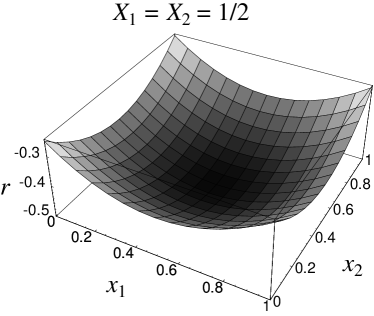
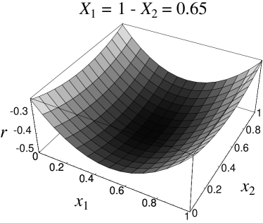
Figure 2: Original Hopfield fitness in the case of two patterns with different $X_{1},X_{2}$.

In the corners of the mutational distance space $\mathcal{S}$, one can see the four degenerate maxima.

The ancestral mean partial distances $\hat{x}_{v}$, at which the maxima of $r-g$ are positioned, are obtained by considering the derivatives of $r-g$. They are given by

$$\hat{x}_{v}=\begin{cases}\frac{1}{2}\pm\frac{1}{2X_{v}}\sqrt{X_{v}^{2}-\mu^{2}}&\text{for $\mu\leq X_{v}$,}\\ \frac{1}{2}&\text{for $\mu\geq X_{v}$.}\end{cases}$$ (50)

For the case of $X_{1}=X_{2}=1/2$, which corresponds to two completely uncorrelated patterns, the ancestral mean partial distances $\hat{x}_{v}$ are shown in figure 3 on the left, alongside the ancestral mean specific distances $\hat{y}^{q}=y^{q}(\hat{x}_{v})$.

Figure 3: Ancestral mean partial distances $\hat{x}_{v}$ (top) and specific distances $\hat{y}^{q}$ (bottom) depending on mutation rates. The original Hopfield fitness (46) for two patterns has been used. Results correspond to uncorrelated patterns ($X_{1}=X_{2}=1/2$, left) and correlated patterns with with $X_{1}=1-X_{2}=0.65$ (right).

For low mutation rates, there are two possible solutions for each of the ancestral mean partial distances $\hat{x}_{v}$, and as the maxima are degenerate, in equilibrium, the population will be centred equally around all of them. However, in the approach to equilibrium, the population might well be predominantly concentrated around one of them, depending on initial conditions. The specific distances $y^{q}$ that are shown correspond to the combination of $\hat{x}_{1}$ and $\hat{x}_{2}$, where both are given by the lower branch. Other combinations yield similar results. For high mutation rates, the population is in the mutation equilibrium with $\hat{x}_{1}=\hat{x}_{2}=1/2$, forming a disordered phase. In the limit of low mutation rates, $\mu\rightarrow 0$, the population is always in the vicinity of one of the patterns (or its complement), such that one of the $\hat{y}^{q}\approx 0\;(1)$, which is completely random with respect to the other pattern, and thus the other $\hat{y}^{q}=1/2$. This is the ordered phase. At the critical mutation rate $\mu_{c}=1/2$, there is a second order phase transition between these two phases, which is a fitness as well as a degradation threshold, corresponding to the infinite derivative of both $\hat{x}_{v}$ at this mutation rate. As the specific distances $y^{q}$ are simply superpositions of the partial distances $x_{v}$, the phase transitions are also visible in the $y^{q}$.

In the correlated case $X_{1}\neq X_{2}$ (figure 3, right), two second order transitions can be identified. At $\mu=X_{1}$, $\hat{x}_{1}$ has a phase transition, whereas at $\mu=X_{2}$, $\hat{x}_{2}$ has a phase transition. The threshold occurring at the lower mutation rate is only a fitness threshold, whereas the one happening at the higher mutation rate is both a fitness and degradation threshold, leading to a totally random population. For $0\leq\mu\leq\min(X_{1},X_{2})$, the population is in an ordered phase, for $\min(X_{1},X_{2})\leq\mu\leq\max(X_{1},X_{2})$, it is in a partially ordered phase, which is ordered with respect to one of the variables, but random with respect to the other. Finally, for $\mu\geq\max(X_{1},X_{2})$, the population is the equidistribution in sequence space. Here again, for low mutation rates the population is close to one of the patterns, but due to the correlation in the chosen patterns, this leads to a non-random overlap with the other pattern. In the uncorrelated case with $X_{1}=X_{2}=1/2$, the two error thresholds coincide, and the partially ordered phase vanishes.

6.2.2 Deviations from the original Hopfield model

Now turn to the question how these phase transitions depend on the particular degeneracy of the fitness functions and consider the quadratic fitness function (47) with negative epistasis (i.e., positive quadratic term) for values of $c\neq-1$.

Figure 4 shows the fitness landscapes for values of $c=-0.9$ and $c=-1.1$ for uncorrelated patterns $X_{1}=X_{2}=1/2$ and correlated patterns with $X_{1}=1-X_{2}=0.65$.

       

       

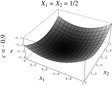
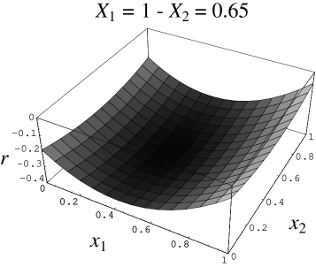
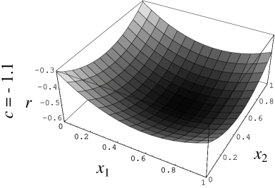
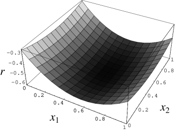
Figure 4: Quadratic Hopfield-type fitness functions (47) with negative epistasis and $c=-0.9$ (top) and $c=-1.1$ (bottom) for an uncorrelated pattern $X_{1}=X_{2}=1/2$ (left) and a correlated pattern with $X_{1}=1-X_{2}=0.65$ (right).

As the pictures indicate, the fitness functions (and thus the behaviour of the system) with the same $|c+1|$ are related by symmetry under $x_{1}\rightarrow 1-x_{1}$ (apart from a constant term, which does not influence the dynamics). Note that in $x_{2}$-direction, the fitness function is independent of $c$. This is because in the sum of the specific distances, the term with $x_{2}$ cancels out, which happens generally in the case of an even number of patterns (i.e., odd $p$) for $\left(\genfrac{}{}{0.0pt}{}{p}{(p+1)/2}\right)$ different variables.

Because in $x_{2}$-direction the fitness is independent of $c$, the solution for the ancestral mean mutational distance $\hat{x}_{2}$ is identical with the solution for the original Hopfield fitness as given in equation (50). So for all values of $c$, the phase transition with respect to $x_{2}$ happens at $\mu=X_{2}$. For $x_{1}$, the solution becomes more complicated, but the inverse function is simpler. It is given by

$$\mu=\frac{2\left[1+c+X_{1}(2\hat{x}_{1}-1)\right]\sqrt{\hat{x}_{1}(1-\hat{x}_{1})}}{2\hat{x}_{1}-1}\,.$$ (51)

The dependence of $\hat{x}_{1}$ on the mutation rate is shown in figure 5 (top).

Figure 5: Ancestral mean partial distance $\hat{x}_{1}$ (top) and specific distances $\hat{y}^{0}$ (thick lines, bottom) and $\hat{y}^{1}$ (thin lines, bottom) depending on mutation rates. The quadratic Hopfield-type fitness (47) with negative epistasis for two patterns and different values of $c$ has been used. Results correspond to uncorrelated patterns $X_{1}=X_{2}=1/2$ (left) and correlated patterns with $X_{1}=1-X_{2}=0.65$ (right). Data are shown for parameter values of $c=-0.9,-0.95,-0.99,-1.01,-1.05,-1.1$ (top to bottom). For clarity, only specific distances $\hat{y}^{q}$ corresponding to $c>-1$ are shown.

For $c\neq-1$, the second order phase transition is smoothed out and thus vanishes. Note that the ambiguity in the solutions that exists in the case $c=-1$ (cf. figure 3), does not exist here, due to the lacking degeneracy of the maxima of the fitness function at $x_{1}=0$ and $x_{1}=1$ (cf. figure 4). At the bottom, figure 5 shows the specific distances $\hat{y}^{q}$, using the lower branch of the solution for $\hat{x}_{2}$ (as shown in figure 3), which show the second order transition in $\hat{x}_{2}$, a fitness threshold. With this combination of solutions, for low mutation rates the population is centred around the sequence complementary to pattern $\boldsymbol{\xi}^{1}$. The general picture for the uncorrelated ($X_{1}=1/2$) and correlated ($X_{1}\neq 1/2$) choice of patterns is very similar, apart from issues like the exact location of the thresholds.

6.3 Quadratic symmetric Hopfield-type fitness with three and more patterns

The behaviour of the system with quadratic symmetric Hopfield-type fitness has been investigated for three, four and five patterns. However, due to the complexity of the analysis for a higher number of patterns, the focus is on the case of three patterns.

For three patterns, the matrix $\boldsymbol{\rho}$ reads

$$\left(\begin{array}[]{cccc}0&0&0&0\\ 0&0&1&1\\ 0&1&0&1\end{array}\right)\;,$$ (52)

thus there are four $X_{v}$ describing the patterns $\boldsymbol{\xi}$, fulfilling $\sum_{v=1}^{4}X_{v}=1$, and four variables $x_{v}\in[0,1]$, describing each sequence. The specific distances with respect to pattern $\boldsymbol{\xi}^{q}$ are given by

$$y^{0} =X_{1}x_{1}+X_{2}x_{2}+X_{3}x_{3}+X_{4}x_{4}\,,$$ (53)

$$y^{1} =X_{1}x_{1}+X_{2}x_{2}+X_{3}(1-x_{3})+X_{4}(1-x_{4})\,,$$ (54)

$$y^{2} =X_{1}x_{1}+X_{2}(1-x_{2})+X_{3}x_{3}+X_{4}(1-x_{4})\;.$$ (55)

Similarly to the case of two patterns, the original Hopfield fitness (46) shall be considered first, and then variations (47) with negative epistasis, but $c\neq-1$. The investigation is done by means of numerical calculations.

6.3.1 Variations of the pattern

For the Hopfield-type fitness, the number of classes in the lumped system is given by $|\mathcal{S}|=\prod_{v=1}^{2^{p}}(N_{v}+1)$. Now consider the case where the patterns are chosen randomly with equal probability for each letter at each site. This results in a multinomial probability distribution for the number of sites $N_{v}$ in each subset (Whittle, 1976),

$$\mathcal{P}(\{N_{1},\ldots,N_{n}\})=\frac{N!}{n^{N}\prod_{v=1}^{n}N_{v}!},$$ (56)

where $n=2^{p}$. The means are given by $\bar{N_{v}}=N/n$ and the variance $\sigma_{v}^{2}=N(n-1)/n^{2}$ such that $N_{v}=N/n+\mathcal{O}(\sqrt{N})$.

If the patterns $\boldsymbol{\xi}^{q}$ for $q=1,\ldots,p$ are chosen randomly (remember $\boldsymbol{\xi}^{0}=00\ldots 0$), the $X_{v}$ are thus given by $X_{v}=2^{-p}+\mathcal{O}\left(\frac{1}{\sqrt{N}}\right)$. So to mimic the case of an infinite sequence length, in which the maximum principle is exact, one has to assume uncorrelated patterns with $X_{v}=2^{-p}$ for all $v=1,\ldots,2^{p}$. However, the maximum principle can also be used to investigate the case of finite sequence length by simulating the finite sequence length through choosing pattern distributions that do not follow exactly the infinite distribution $X_{v}=2^{-p}$, but vary around this mean value with a variance according to the sequence length to be simulated. Practically, patterns corresponding to finite sequence length $N$ have been obtained by choosing for the $3N$ sites entries $0$ or $1$ with probability 1/2 at each site, and counting the number of sites $N_{v}$ in each class $\Lambda_{v}$, similarly to the example pattern given in equation (8). Thus although the patterns were chosen randomly, they are correlated due to the finite sequence length.

As shall be seen in the following, these correlations do account for some interesting additional features. However, focus first on the case of a genuinely infinite sequence length with $X_{v}=2^{-p}$ for all $v$.

6.3.2 The case of infinite sequence length

Original Hopfield fitness ($c=-1$).

The results for the case of three, four and five patterns with original Hopfield fitness (46) and uncorrelated patterns ($X_{v}=2^{-p}$ for all $v$, corresponding to random patterns for infinite sequence length) look exactly like those for two patterns shown in figure 3 (left).

The solutions for the different $x_{v}$ all coincide. For small mutation rates $\mu<1/2$, there are again two degenerate solutions for each $x_{v}$, which can be combined in multiple ways for the different $x_{v}$, yielding any of the patterns or their complementary sequences. At $\mu=1/2$, there is a second order phase transition, which is a fitness and degradation threshold. For small mutation rates, the population is centred around one of the patterns, say $\boldsymbol{\xi}^{q_{c}}$, and therefore $y^{q_{c}}<1/2$, whereas it is completely random with respect to the other patterns, yielding $y^{q}=1/2$ for $q\neq q_{c}$.

Deviations from the original Hopfield fitness ($c\neq-1$).

Figure 6: Ancestral mean partial distances $\hat{x}_{v}$ (top) and specific distances $\hat{y}^{q}$ (bottom) depending on mutation rates. The quadratic Hopfield-type fitness (47) with negative epistasis for three patterns with $c=-0.9$ (left) and $c=-1.1$ (right) has been used. Results correspond to uncorrelated patterns for infinite sequence length ($X_{v}=1/4\;\forall v$).

Figure 6 shows the ancestral mean partial distances $\hat{x}_{v}$ and specific distances $\hat{y}^{q}$ for the quadratic Hopfield-type fitness (47) with negative epistasis for different values of $c$ in the case of three patterns. Data for four patterns look very similar (not shown). As $c$ deviates from $-1$, the solutions for the $x_{v}$ do not coincide, and the phase transition becomes a first order fitness threshold, at which all four partial distances $\hat{x}_{v}$ jump, but it is no more a degradation threshold. So contrary to the case of two patterns, where $\hat{x}_{2}$ is independent of $c$ and the error threshold in $\hat{x}_{1}$ is smoothed out by $c$ deviating from $-1$, here the threshold concerns all four partial distances $\hat{x}_{v}$ and is sharpened to first order by $c\neq-1$.

For $c\neq-1$, the degeneracy between the patterns and their complements is lifted, and thus for mutation rates below the threshold, there are only $p+1$ different solutions, correlated with the patterns for $c<-1$, and with their complements for $c>-1$. For clarity, only one of the solutions is shown in figure 6.

Furthermore, the critical mutation rate decreases with increasing $|c+1|$. The dependence of the critical mutation rate $\mu_{c}$ on the value of $c$ for $p=2,3$ is shown in figure 7.

Figure 7: The critical mutation rate $\mu_{c}$ depending on the value of $c$. The quadratic Hopfield-type fitness (47) with negative epistasis for three and four patterns has been used. Results correspond to uncorrelated patterns simulating infinite sequence length.

At $c=-5/4$ and $c=-3/4$, the critical mutation rate is $\mu_{c}=0$, and for values of $c\notin[-5/4,-3/4]$, there are no first order error thresholds for either $p=2$ or $p=3$. This goes in line with a different sequence becoming optimal at $\mu=0$ for these values of $c$.

However, for $p=3$, there is an additional line of second order error thresholds, that approaches $\mu_{c}=1/4$ as $|c+1|$ grows. Preliminary results for $p=4$ indicate, that in that case the second order line does not occur. It might thus be conjectured that the existence of the second order error threshold line depends on the number of patterns being even or odd (remember that for $p=1$ it does exist).

This is an interesting result, as for all previously investigated Hopfield-type fitness functions (which are limited to the original Hopfield fitness and a Hopfield-type truncation selection as far as the author is aware), the existence of error thresholds has been reported.

6.3.3 The case of correlated patterns simulating a finite sequence length

Figure 8: Ancestral mean partial and specific distances, $\hat{x}_{v}$ and $\hat{y}^{q}$, depending on mutation rates. The original Hopfield fitness (46) for three patterns has been used. Results correspond to two typical examples of random, but correlated patterns chosen for sequences of lengths $N=1000$ (left), $N=300$ (middle) and $N=100$ (right), specified at the top of each graph as $(X_{1},X_{2},X_{3},X_{4})$.

Figure 8 shows some cases of the ancestral mean partial and specific distances, $\hat{x}_{v}$ and $\hat{y}^{q}$, for the original Hopfield fitness (46) with three patterns, which are randomly chosen sequences of finite length. The correlations between the patterns (and thus the variations of the $X_{v}$) are characteristic for the sequence length. The six cases of patterns shown here are typical examples for the sequence lengths considered. In the case of long sequences ($N=1000$), the deviations of the patterns from the infinite sequence limit $X_{1}=X_{2}=X_{3}=X_{4}$ are small, and grow with decreasing sequence length. These correlations that are introduced into the system have the same effect as a choice of correlated patterns in the case of two patterns, such that the single critical mutation rate in the case of infinite sequence length is split up into two critical mutation rates, at each of which two of the $x_{v}$ show threshold behaviour. For short sequence length ($N=100$), it can be seen that, particularly at the smaller critical mutation rate, the threshold is smoothed out.

Figure 9: Ancestral mean partial and specific distances, $\hat{x}_{v}$ and $\hat{y}^{q}$, depending on mutation rates. The Hopfield-type fitness (47) with negative epistasis for three patterns and $c=-1.1$ has been used. Results correspond to the patterns used in figure 8.

In figure 9, the ancestral mean partial and specific distances, $\hat{x}_{v}$ and $\hat{y}^{q}$, corresponding to the same patterns as in figure 8 are shown for the quadratic Hopfield-type fitness (47) with negative epistasis and $c=-1.1$. For long sequence length, these look very similar to the results for infinite sequence length (cf. figure 6), showing clearly the single first order phase transition. For shorter sequence lengths, they become more and more smoothed out, such that at $N=300$, roughly only every other pattern that was simulated shows an error threshold, whereas for $N=100$, in the vast majority of cases, there is no threshold. Note that this effect is present even though the finite sequence length was only simulated by choosing the patterns accordingly, so it is a feature of the model with correlated patterns.

6.4 Summary of the results for Hopfield-type fitness

In this section, the quadratic symmetric Hopfield-type fitness given in equation (47) with negative epistasis (i.e., positive quadratic term) was investigated for a small number of patterns. The results for the original Hopfield fitness ($c=-1$) have been compared with those for the generalised quadratic Hopfield-type fitness ($c\neq 1$). Furthermore, both uncorrelated patterns ($X_{v}=2^{-p}$ for all $v$), corresponding to an infinite sequence length, and correlated patterns ($X_{v}\neq 2^{-p}$), simulating a finite sequence length, were considered. For two patterns, an analytical treatment was possible, making all values of the $X_{v}$ accessible, whereas the case of three or more patterns was treated numerically due to the larger number of variables. This means that apart from the uncorrelated choice of pattern ($X_{v}=2^{-p}$), which was investigated for three, four and five patterns, only some correlated combinations for three patterns with $X_{v}\neq 2^{-p}$ were investigated, some typical examples of which are shown in section 6.3. The results are summarised as follows:

• Original Hopfield fitness ($c=-1$):

  • For uncorrelated patterns, there is one second order error threshold for all $x_{v}$ at $\mu_{c}=1/2$ (investigated $p=1,2,3,4$).

  • For correlated patterns, there are two second order error thresholds, each for half of the $x_{v}$ (investigated $p=1,2$).

• Hopfield-type fitness with $c\neq-1$:

  • For uncorrelated patterns, there is a first order error threshold only on a restricted range of $c$ ($p=1:$ no first order threshold, $p=2,3:c\in[-5/4,-3/4]$).
    For an even number of patterns ($p=1,3$), there is an additional second order error threshold for any $|c+1|\geqslant\Delta c$ ($p=1:\Delta c=0$, $p=3:\Delta c\approx 0.145$). This error threshold does not exist for the investigated cases of an odd number of patterns ($p=2,4$).

  • For correlated patterns, at $p=1$, there is one second order threshold, the other one, which is present for the original Hopfield fitness, is smoothed out. At $p=2$, there is up to one first order threshold, smoothed out for more strongly correlated patterns (corresponding to shorter sequence length).

The evaluation the Hopfield-type fitness was limited to the cases of rather small numbers of patterns, simply because an increase in the number of patterns makes the evaluation more complex. However, the Hopfield-type fitness was chosen as a potentially realistic fitness because of its ruggedness that can be tuned by the number of patterns chosen. The simple cases considered here probably do not show as high a degree of ruggedness as one would expect for realistic fitness functions. However, the results described here already indicate some features that are common for all numbers of patterns investigated here, and some that depend on whether the number of patterns is odd or even. It would be very interesting to establish whether these results generalise to an arbitrary number of patterns.

Furthermore, the concept of partitioning the set of sites into subsets, which was introduced to analyse the Hopfield-type fitness, is very interesting. One could imagine a different interpretation for this by classifying sites according to the selection strength they evolve under. Some of the behaviour identified for the Hopfield system could also occur in such a setting: At intermediate mutation rates, partially ordered phases could exist, such that sites that evolve under weak selection have passed their error threshold and the population is in a phase that is disordered with respect to these sites, whereas at sites that are subject to strong selection the order is still maintained.

7 Conclusion

The present work has been concerned with the investigation of a deterministic mutation–selection model in the sequence space approach, using a time-continuous formulation. Important observables in these mutation–selection models are the population and ancestral distributions $\boldsymbol{p}$ and $\boldsymbol{a}$, and means with respect to these distributions, in particular the population mean fitness $\bar{r}$ and the ancestral mean genotype $\boldsymbol{\hat{x}}$. In equilibrium, $\boldsymbol{p}$ is given by the right Perron-Frobenius eigenvector of the time-evolution operator $\boldsymbol{H}$, whereas the ancestral distribution is given by the product of both right and left PF eigenvectors $\boldsymbol{p}$ and $\boldsymbol{z}$, $a_{i}=z_{i}p_{i}$.

Types have been modelled as two-state sequences. As mutation model, the single step mutation model was used, whereas selection was modelled by Hopfield-type fitness functions, using the similarity of a sequence to a number of patterns to determine its fitness. This allows for a more rugged fitness landscape, and the complexity of the fitness can be tuned by the number of patterns.

The large number of types that arise in the sequence space approach have been lumped into classes of types, labelled by the partial distances $d_{v}$ introduced in section 4 as a generalisation of the Hamming distance. With this, the maximum principle as developed by Baake et al. (2005) can be applied to the case of Hopfield-type fitness functions as done in section 5, see also Garske (2005), treating two- and four-state sequences.

In section 6, the maximum principle derived in section 5 was used to investigate the phenomenon of the error threshold. These error thresholds can be detected with the maximum principle, because the delocalisation of the population distribution manifests itself as a jump (or at least an infinite derivative with respect to the mutation rate) of the ancestral mean genotype $\boldsymbol{\hat{x}}$, the maximiser. Not all fitness functions give rise to error thresholds, and as the error thresholds were first described for a model with highly unrealistic fitness function, it has been argued that they might be an artifact of this rather than a biologically relevant phenomenon. It is therefore clearly necessary to investigate more complex fitness functions with respect to this phenomenon.

Here, quadratic Hopfield-type fitness functions with small numbers of patterns have been investigated. For the original Hopfield fitness, the results for all investigated numbers of patterns are identical. However, if the fitness differs from the original Hopfield fitness, different behaviours are observed for different numbers of patterns. In the case of uncorrelated patterns, corresponding to random patterns chosen for infinite sequence length, the observed features seem to depend on whether the number of patterns is odd or even. Because for correlated patterns, only the cases of two and three patterns were investigated, and found to behave differently, it would be interesting to see how these results generalise to a higher number of patterns.

In the original Hopfield fitness, error thresholds were observed for all choices of patterns. This is not true for a generalised Hopfield-type fitness. For instance, for a Hopfield-type fitness with positive epistasis no thresholds were observed, going in line with the results for permutation-invariant fitness. But also for Hopfield-type fitness functions with negative epistasis, there are not necessarily any thresholds, if the fitness deviates too much from the original Hopfield fitness, challenging the commonly held notion that more complex fitness functions all tend to display error threshold behaviour. The complexity and ruggedness of the original Hopfield fitness have been investigated (Amit et al., 1985a, b) and found to be good candidates for realistic fitness functions (Leuthäusser, 1987; Tarazona, 1992). However, these results do not necessarily transfer to the generalised Hopfield-type fitness functions, and therefore it would be very useful to study these properties of a generalised Hopfield-type fitness functions to analyse which of these factors are responsible for generating the thresholds.

References

- Amit et al. (1985a) Amit, D. J., Gutfreund, H., Sompolinsky, H., 1985a. Spin-glass models of neural networks. Physical Review A 32 (2), 1007–1018.
- Amit et al. (1985b) Amit, D. J., Gutfreund, H., Sompolinsky, H., 1985b. Storing infinite numbers of patterns in a spin-glass model of neural networks. Physical Review Letters 55 (14), 1530–1533.
- Baake et al. (2005) Baake, E., Baake, M., Bovier, A., Klein, M., 2005. An asymptotic maximum principle for essentially linear evolution models. Journal of Mathematical Biology 50 (1), 83–114.
- Baake et al. (1997) Baake, E., Baake, M., Wagner, H., 1997. Ising quantum chain is equivalent to a model of biological evolution. Physical Review Letters 78 (3), 559–562, erratum, Physical Review Letters 79 (1997), 1782.
- Baake and Gabriel (2000) Baake, E., Gabriel, W., 2000. Biological evolution through mutation, selection, and drift: An introductory review. In: Stauffer, D. (Ed.), Annual Reviews of Computational Physics VII. World Scientific, Singapore, pp. 203–264.
- Baake and Wagner (2001) Baake, E., Wagner, H., 2001. Mutation-selection models solved exactly with methods of statistical mechanics. Genetical Research 78, 93–117.
- Boerlijst et al. (1996) Boerlijst, M. C., Bonhoeffer, S., Nowak, M. A., 1996. Viral quasi-species and recombination. Proceedings of the Royal Society of London, Series B 263 (1376), 1577–1584.
- Bonhoeffer and Stadler (1993) Bonhoeffer, S., Stadler, P. F., 1993. Error thresholds on correlated fitness landscapes. Journal of Theoretical Biology 164 (3), 359–372.
- Bürger (2000) Bürger, R., 2000. The Mathematical Theory of Selection, Recombination, and Mutation. Wiley, Chichester.
- Campos et al. (2002) Campos, P. R. A., Adami, C., Wilke, C. O., 2002. Optimal adaptive performance and delocalization in NK fitness landscapes. Physica A 304 (3–4), 495–506.
- Crotty et al. (2001) Crotty, S., Cameron, C. E., Andino, R., 2001. RNA virus error catastrophe: Direct molecular test by using ribavirin. Proceedings of the National Academy of Sciences of the USA 98 (12), 6895–6900.
- Crow and Kimura (1970) Crow, J. F., Kimura, M., 1970. An Introduction to Population Genetics Theory. Harper & Row, New York.
- Domingo et al. (1996) Domingo, E., Escarmis, C., Sevilla, N., Moya, A., Elena, S. F., Quer, J., Novella, I. S., Holland, J. J., 1996. Basic concepts in RNA virus evolution. FASEB Journal 10 (8), 859–864.
- Domingo and Holland (1988) Domingo, E., Holland, J. J., 1988. High error rates, population equilibrium, and evolution of RNA replication systems. In: Domingo, E. (Ed.), RNA Genetics. Vol. 3. CRC Press, Boca Raton, p. 3.
- Domingo and Holland (1997) Domingo, E., Holland, J. J., 1997. RNA virus mutations and fitness for survival. Annual Review of Microbiology 51, 151–178.
- Eigen (1971) Eigen, M., 1971. Selforganization of matter and the evolution of biological macromolecules. Naturwissenschaften 58 (10), 465–523.
- Eigen (1993) Eigen, M., 1993. Viral quasispecies. Scientific American 269 (1), 42–49.
- Eigen and Biebricher (1988) Eigen, M., Biebricher, C. K., 1988. Sequence space and quasispecies evolution. In: Domingo, E. (Ed.), RNA Genetics. Vol. 3. CRC Press, Boca Raton, pp. 211–245.
- Eigen et al. (1989) Eigen, M., McCaskill, J., Schuster, P., 1989. The molecular quasi-species. Advances in Chemical Physics 75, 149–263.
- Ewens (2004) Ewens, W. J., 2004. Mathematical Population Genetics, 2nd Edition. Springer, New York.
- Franz and Peliti (1997) Franz, S., Peliti, L., 1997. Error threshold in simple landscapes. Journal of Physics A 30 (13), 4481–4487.
- Franz et al. (1993) Franz, S., Peliti, L., Sellitto, M., 1993. An evolutionary version of the random energy model. Journal of Physics A 26 (23), L1195–L1199.
- Garske (2005) Garske, T., 2005. Mutation–selection models of sequence evolution in population genetics. Ph.D. thesis, The Open University, Milton Keynes, UK.
- Garske and Grimm (2004a) Garske, T., Grimm, U., 2004a. Maximum principle and mutation thresholds for four-letter sequence evolution. Journal of Statistical Mechanics: Theory and Experiment P07007, (Preprint q-bio.PE/0406041).
- Garske and Grimm (2004b) Garske, T., Grimm, U., 2004b. A maximum principle for the mutation–selection equilibrium of nucleotide sequences. Bulletin of Mathematical Biology 66 (3), 397–421, (Preprint physics/0303053).
- Hamming (1950) Hamming, R. W., 1950. Error detecting and error correcting codes. The Bell System Technical Journal 26 (2), 147–160.
- Hermisson et al. (2002) Hermisson, J., Redner, O., Wagner, H., Baake, E., 2002. Mutation selection balance: Ancestry, load, and maximum principle. Theoretical Population Biology 62, 9–46.
- Hermisson et al. (2001) Hermisson, J., Wagner, H., Baake, M., 2001. Four-state quantum chain as a model of sequence evolution. Journal of Statistical Physics 102 (1/2), 315–343.
- Higgs (1994) Higgs, P., 1994. Error thresholds and stationary mutant distributions in multilocus diploid genetics models. Genetical Research Cambridge 63 (1), 63–78.
- Holland et al. (1990) Holland, J. J., Domingo, E., de la Torre, J. C., Steinhauer, D. A., 1990. Mutation frequencies at defined single codon sites in vesicular stromatitis-virus and poliovirus can be increased only slightly by chemical mutagenesis. Journal of Virology 64 (8), 3960–3962.
- Hopfield (1982) Hopfield, J. J., 1982. Neural networks and physical systems with emergent collective computational abilities. Proceedings of the National Academy of Sciences of the USA 79 (8), 2554–2558.
- Huynen et al. (1996) Huynen, M. A., Stadler, P. F., Fontana, W., 1996. Smoothness within ruggedness: the role of neutrality in adaptation. Proceedings of the National Academy of Sciences of the USA 93 (1), 397–401.
- Karlin (1966) Karlin, S., 1966. A First Course in Stochastic Processes. Academic Press, New York.
- Kauffman and Levin (1987) Kauffman, S., Levin, S., 1987. Towards a general theory of adaptive walks on rugged landscapes. Journal of Theoretical Biology 128, 11–45.
- Kemeny and Snell (1960) Kemeny, J. G., Snell, J. L., 1960. Finite Markov Chains. Van Nostrand Reinhold Company, New York.
- Leuthäusser (1987) Leuthäusser, I., 1987. Statistical mechanics of Eigen’s evolution model. Journal of Statistical Physics 48 (1/2), 343–360.
- Loeb et al. (1999) Loeb, L. A., Essigmann, J. M., Kazazi, F., Zhang, J., Rose, K. D., Mullins, J. I., 1999. Lethal mutagenesis of HIV with mutagenic nucleoside analogs. Proceedings of the National Academy of Sciences of the USA 96, 1492–1497.
- Nowak and Schuster (1989) Nowak, M., Schuster, P., 1989. Error thresholds of replication in finite populations. Mutation frequencies and the onset of Muller’s ratchet. Journal of Theoretical Biology 137 (4), 375–395.
- Ohta and Kimura (1973) Ohta, T., Kimura, M., 1973. A model of mutation appropriate to estimate the number of electrophoretically detectable alleles in a finite population. Genetical Research 22, 201–204.
- Peliti (2002) Peliti, L., 2002. Quasispecies evolution in general mean-field landscapes. Europhysics Letters 57 (5), 745–751.
- Reidys et al. (2001) Reidys, C., Forst, C. V., Schuster, P., 2001. Replication and mutation on neutral networks. Bulletin of Mathematical Biology 63 (1), 57–94.
- Reidys and Stadler (2002) Reidys, C. M., Stadler, P. F., 2002. Combinatorial landscapes. SIAM Review 44 (1), 3–54.
- Rumschitzky (1987) Rumschitzky, D. S., 1987. Spectral properties of Eigen’s evolution matrices. Journal of Mathematical Biology 24, 667–680.
- Sierra et al. (2000) Sierra, S., Dávila, M., Lowenstein, P. R., Domingo, E., 2000. Response of foot-and-mouth disease virus to increased mutagenesis: Influence of viral load and fitness in loss of infectivity. Journal of Virology 74 (18), 8316–8323.
- Talagrand (2003) Talagrand, M., 2003. Spin Glasses: A Challenge for Mathematicians. Springer, Berlin.
- Tarazona (1992) Tarazona, P., 1992. Error thresholds for molecular quasispecies as phase transitions: From simple landscapes to spin-glass models. Physical Review A 45 (8), 6038–6050.
- van Lint (1982) van Lint, J. H., 1982. Introduction to Coding Theory. Springer, Berlin.
- Whittle (1976) Whittle, P., 1976. Probability. Wiley, London.
- Wiehe (1997) Wiehe, T., 1997. Model dependency of error thresholds: The role of fitness functions and contrasts between finite and infinite sites models. Genetical Research Cambridge 69, 127–136.
- Wiehe et al. (1995) Wiehe, T., Baake, E., Schuster, P., 1995. Error propagation in reproduction of diploid organisms. A case study on single peaked landscapes. Journal of Theoretical Biology 177 (1), 1–15.