Efficient spike-sorting of multi-state neurons using inter-spike intervals information

Abstract

We demonstrate the efficacy of a new spike-sorting method based on a Markov Chain Monte Carlo (MCMC) algorithm by applying it to real data recorded from Purkinje cells (PCs) in young rat cerebellar slices. This algorithm is unique in its capability to estimate and make use of the firing statistics as well as the spike amplitude dynamics of the recorded neurons. PCs exhibit multiple discharge states, giving rise to multimodal interspike interval (ISI) histograms and to correlations between successive ISIs. The amplitude of the spikes generated by a PC in an “active” state decreases, a feature typical of many neurons from both vertebrates and invertebrates. These two features constitute a major and recurrent problem for all the presently available spike-sorting methods. We first show that a Hidden Markov Model with 3 log-Normal states provides a flexible and satisfying description of the complex firing of single PCs. We then incorporate this model into our previous MCMC based spike-sorting algorithm [PouzatEtAl_2004, , Pouzat et al, 2004, J. Neurophys. 91, 2910-2928] and test this new algorithm on multi-unit recordings of bursting PCs. We show that our method successfully classifies the bursty spike trains fired by PCs by using an independent single unit recording from a patch-clamp pipette.

1 Introduction

Multi-site extracellular recordings are extensively used by laboratories that aim at studying neuronal populations activity and a variety of recently developed technologies enable the experimentalist to do so in many preparations: cultures GrossEtAl_1993 , GrossEtAl_1997 , slices OkaEtAl_1999 , EgertEtAl_2002 , in vivo DrakeEtAl_1988 , NicolelisEtAl_1997 , BakerEtAl_1999 , CsicsavariEtAl_2003 . But in order to be really informative and fully exploitable, such recordings require the difficult spike-sorting problem to be solved: the resolution of a mixture of activities into well separated individual spike trains. This problem has an already long history Lewicki_1998 , but has not yet received any fully satisfying solution BrownEtAl_2004 , Buzsaki_2004 . In particular, until recently PouzatEtAl_2004 , Pouzat_2005 , all of the available methods made exclusively use of the information provided by the waveform of individual spikes, ignoring that of their occurrence times. Many neurons have however fairly reproducible firing features that can often be summarized by their inter-spike interval (ISI) probability density. This temporal information can greatly improve classification performance and allows the investigator to take into account the dependence of the spike amplitude upon the ISI, like for instance during a burst (where a spike amplitude reduction is typically observed on an extracellular electrode as well as on an intracellular one).

In that context, we recently proposed a new Bayesian method based on a Markov Chain Monte Carlo (MCMC) approach PouzatEtAl_2004 , Pouzat_2005 . This method is built on a data generation model that includes both a description of non Poisson neuronal discharge statistics and a description of spike waveform dynamics. In these papers, we chose a single log-Normal density to model individual ISIs distributions. It is nevertheless clear that this is not the only model that can be considered: the MCMC framework allows the experimentalist to use the model that is best supported by the data from the neuronal type he is studying. In particular, when one is dealing with neurons exhibiting several states resulting in bursty discharges the unimodal log-Normal density is not appropriate anymore, as observed for example in thalamic relay cells McCormick_1998 and in cerebellar Purkinje cells (PCs) LoewensteinEtAl_2005 .

The primary goal of the present paper is to show how our spike-sorting method, modified to take into account such multi-state neurons, performs on real data that would make any other automatic method fail. We chose a challenging data set recorded from cells firing bursts of spikes. Such data could be obtained in young rat cerebellar slices by applying a multi-site electrode along the PCs layer in the presence of the group I metabotropic glutamate receptor (mGluR1) agonist (S)-3,5-dihydroxyphenylglycine (DHPG). In these pharmacological conditions, PCs fire bursts of two or more action potentials (APs) with dramatically decreasing amplitudes (eg. 50%), in alternance with long periods of silence (on the order of 1 minute) NetzebandEtAl_1997 .

2 Methods

2.1 Experimental procedure

Slices preparation and loose cell-attached patch-clamp recording were done as previously described PouzatHestrin_1997 . Sagittal slices (180 $\mu$m thick) were taken from the vermis of cerebella from rats aged 11-14 days. Single and multiple unit(s) recordings were made from PCs in these slices visualized through a 63X objective in an upright microscope equipped with Nomarski optics (Axioscope, Carl Zeiss, Germany). These conditions allowed easy resolution of the various layers and cell types within the cerebellar cortex. During recording, the slices were maintained at room temperature (20-22 °C). They were continuously perfused with BBS which contained (mM): 130 $NaCl$, 2.5 $KCl$, 2 $CaCl_{2}$, 1 $MgCl_{2}$, 1.3 $NaH_{2}PO_{4}$, 26 $NaHCO_{3}$ and 25 glucose. This solution was continuously bubbled with a mixture of 95% $O_{2}$ and 5% $CO_{2}$, the solution pH being thus kept at 7.4.

The mGluR1 agonist DHPG (40 $\mu$M) was applied dissolved in the bathing solution. All the recordings analyzed in this paper were made in these conditions. DHPG was purchased from Tocris Neuramin Ltd (Bristol, UK). It was dissolved in distilled water at a concentration of 5 mM. The DHPG stock solution was stored frozen, and the final concentration was obtained by diluting the stock solution in the saline, just before its use in the experiment. Note that spontaneous bursting also occurred without DHPG at this age, but less systematically.

Single unit recordings were performed in loose cell-attached using a glass micropipette filled with the following solution (mM): 145 $NaCl$, 2.5 $KCl$, 2 $CaCl_{2}$, 1 $MgCl_{2}$ , 10 HEPES acid. Pipette resistance ranged from 2 to 4 M$\Omega$. The pipette was positioned in loose cell-attached on the soma of a PC. It was connected to a patch-clamp amplifier (Axoclamp 2B, Axon Instruments Inc., USA). This amplifier was connected to one of the 8 channels of two 4-channel differential AC amplifiers (AM systems, model 1700, Carlsborg, WA), also used for multi-unit data recordings (see below). The signal was band-pass filtered between 300 and 5000 Hz and amplified 1000 times. Such single unit recordings were performed in two types of experiments. First, they were made alone in order to gather several examples of individual PCs spike trains during spontaneous activity. Second, they were made together with multiple units recordings where they served as a reference recording to which the spike-sorting output was compared.

Multi-unit recordings were performed using silicon probes (also called “multi-site electrodes” in the sequel) kindly provided by the Center for Neural Communication Technology of the University of Michigan. A schematic drawing of the tip (first 4 recording sites) of the probe is shown in Fig. 5. The 16 recording sites are linearly placed on the electrode 50 $\mu$m apart . This electrode was positioned along the PCs layer. The spontaneous spiking activities of these PCs could routinely be recorded on the first 8 sites of the electrode, with an excellent signal-to-noise ratio (see Fig. 5B1, B2, C1, C2 for some examples). The analysis detailed in the present paper was made on the first 4 recording sites. A glass micropipette was positioned in loose cell-attached on the soma of one of the PCs whose spontaneous activity was recorded by the multi-site electrode.

The multi-site electrode was connected to a custom made impedance matching preamplifier. The preamplifier was connected to the two 4-channel differential AC amplifiers mentioned above. The signals were bandpass filtered between 300 and 5000 Hz and amplified 2000 times. All data were acquired at 15 kHz using a 16 bit A/D card (PD2MF-64-500/16H, United Electronics Industries, Watertown, MA) and stored on disk for subsequent analysis.

2.2 Data analysis

2.2.1 Events detection and representation

Multi-unit data. Data recorded on the first 4 recording sites of the multi-site electrode were analyzed. A first set of large events were detected as local maxima with a peak value exceeding a preset high threshold (5 times the standard deviation (SD) of the whole trace), and normalized (peak amplitude, at 1, temporal average, at 0) to give a “spike template”. Each trace was then filtered with this template (by convolution with the template in reversed time order). Events were detected on the filtered trace as local maxima whose peak value exceeded a preset threshold (a multiple of the SD of the filtered trace). After detection, each event was described by its occurrence time and its peak amplitude measured on 4 recording sites. To simplify calculations and reduce the complexity of our algorithm, the peak amplitude(s) were “noise whitened” as described in PouzatEtAl_2002 (see also SpikeOMaticTutorial 1). A spike detected on a given recording site can be seen on its immediate neighbouring sites ($50\mu m$ apart) with reduced amplitudes, but never on further sites. This is consistent with an exponential decay of the signal with decay constant $\leavevmode\nobreak\ 30\mu m$ GrayEtAl_1995 , SegevEtAl_2004 .

Single unit data. For data recorded by the glass micropipette, events were detected the same way. Each event was described by its occurrence time and its peak amplitude. We normalized the peak amplitudes of the spikes by the SD of 2000 noise “peak” amplitudes taken in the same recording. When single unit data were recorded together with multi-unit data, events detected on the micropipette trace were described by their occurrence times only.

2.2.2 Data generation model for statistical inference

To perform spike-sorting our algorithm makes statistical inference on the parameters of the data generation model described in this section. This model is based on the following assumptions:

1. The sequence of spike times from a given neuron is a realization of a Hidden Markov point process CamprouxEtAl_1996 , GucluBolanowski_2004 .

2. The spike amplitudes generated by a neuron depend on the elapsed time since the previous spike of this neuron.

3. The measured spike amplitudes are corrupted by a Gaussian white noise which sums linearly with the spikes and is statistically independent of them.

Assumptions 2 and 3 are identical to those made in PouzatEtAl_2004 , Pouzat_2005 . Assumption 3 requires a prior noise whitening of the data PouzatEtAl_2002 . In assumption 1, the homogeneous renewal point process assumption that was made in PouzatEtAl_2004 , Pouzat_2005 is changed into the more complex one of a hidden Markov point process (see below and in Appendix sec.A.1.1). Our data generation model can be divided in two parts that respectively rely on assumptions 1 and 2 which are presented next.

Inter-spike interval density

We resort to a Hidden Markov Model (HMM) with 3 states to account for the empirical ISI density of the recorded cells. In this HMM context, we can see a sequence of ISIs (a spike train) produced by a given neuron as the observable output of a “hidden” sequence of “states” of this neuron (this denomination arises from the fact that the state in which the neuron is, is not directly observable from the data). The probability density from which each ISI is drawn depends on the underlying state. In our particular implementation, the ISI density of each state is a log-Normal density characterized by 2 parameters: a scale parameter s (in seconds) and a shape parameter $\sigma$ (dimensionless). With this notation, the general formula for the probability density function of the log-Normal distribution is:

$$f(isi)=\frac{1}{isi\cdot\sigma\cdot\sqrt{2\pi}}\cdot\exp\left(-\frac{1}{2}\cdot(\frac{\log(\frac{isi}{s})}{\sigma})^{2}\right)$$ (1)

The log-Normal density is a relevant alternative to the exponential density usually used to model spike trains. It is unimodal, exhibits a refractory period, rises fast and decays slowly.

After the generation of each event, a “transition” to any of the three possible states is performed stochastically. In addition to the 6 parameters for the 3 log-Normal densities mentioned above, we have therefore to consider the transition matrix $\left(q_{ij}\right)$ between these states, which contains another 6 parameters. We thus have 12 parameters to specify the ISI density for each neuron.

A scheme summarizing this model is shown in Fig. 1A. In a spike train, each event (ISI) is generated by one of the 3 possible probability densities according to the state in which the neuron is: if the neuron is in state 1 (resp. 2, 3) it generates a short (resp. intermediate, long) ISI from the red (resp. blue, green) density. The transition from a given state to any other, including itself, is possible, as indicated by the different arrows between states. In the sequel we will constantly refer to the same color code for the states of single unit data: state 1 in red, state 2 in blue, state 3 in green. They will be also called “short”, “intermediate” and “long” states respectively. A more formal presentation of the HMM is to be found in sec. A.1.1 of the Appendix.

Spike amplitude dynamics

We use here the same spike amplitude dynamics as in PouzatEtAl_2004 , Pouzat_2005 . We consider events described by their occurrence time and their peak amplitude measured on 1 (single site recordings) or 4 recording sites (multi-site recordings). We model the dependence of the amplitude on the ISI by an exponential relaxation FeeEtAl_1996b :

$$A(isi)=P\cdot(1-\delta\cdot\exp(-\lambda\>isi))$$ (2)

where isi is the ISI, $\lambda$ is the inverse of the relaxation time constant (measured in 1/s), $P$ is the vector of the maximal amplitude of the event on each recording site (this is a 4-dimension, resp. 1-dimension, vector for multi-site, resp. single site, recordings) and $\delta$ is the dimensionless maximal modulation. This model implies that the modulation of the amplitudes of an event is the same on the different recording sites. This is an important feature of the amplitude modulation observed experimentally GrayEtAl_1995 . Added to the 12 parameters used for the ISIs, the number of parameters per neuron in our model amounts to 18 for multi-site recordings and 15 for single site recordings.

2.2.3 The Markov Chain Monte Carlo approach

We have shown in our previous papers that the spike-sorting problem with a data generation model similar to the one presented here can be viewed as a one dimensional Potts spin-glass in a random magnetic field PouzatEtAl_2004 , Pouzat_2005 . This analogy allowed us to tailor the Dynamic Monte Carlo algorithms developed by physicists NewmanBarkema_1999 , FrenkelSmit_2002 and the Markov Chain Monte Carlo (MCMC) developed by statisticians RobertCasella_1999 , Liu_2001 for analogous problems to our particular needs. In essence the statistical inference in our case relies on the construction of a Markov chain (not to be mistaken for the HMM which is modeling the ISI density) whose space $\mathcal{S}$ is the product of two spaces: the space of the model parameters defined in our data generation model ( and presented in the previous section) and the space of spike train configurations, where a configuration is defined by specifying a neuron of origin (a “label”) and a neuron state for each spike. The latter, neuron state, is the new model ingredient introduced in the present paper (section LABEL:par:Inter-spike-interval-density). Thus a state of our Markov chain in this space is determined by two vectors: vector $\theta$ of model parameters (a $18\cdot K$, resp.$15\cdot K$, dimensional vector for multi-site, resp. single site, recordings, where $K$ is the number of neurons, see Methods, sec. 2.2.2) and vector $C$ of the configuration, specifying a label and a neuron state for each spike (a $2\cdot N$ dimensional vector, where $N$ is the number of detected spikes being analyzed). The construction of this Markov chain is done in such a way that it samples our space $\mathcal{S}$ from the posterior density of the model parameters and configurations given the data $Y$, noted $\pi_{post}(\theta,C\mid Y)$: at each step $t$ of the algorithm a new state $\left[\theta^{\left(t\right)},C^{\left(t\right)}\right]$ of the Markov chain (not to be mistaken for the neuron states of the HMM used to model the ISI density) is generated from the state at step $t-1$, $\left[\theta^{\left(t-1\right)},C^{\left(t-1\right)}\right]$, according to the procedure described in Appendix, sec. A.1.2. The new components of the algorithm are the generation of the neuron states of the HMM (when generating the new configuration) and the generation of the transitions $q_{ij}$ between these neuron states (which are components of the vector $\theta$ of parameters), using a Dirichlet distribution RobertCasella_1999 . This way of generating a new state from the previous one ensures that the Markov chain converges to a unique stationary distribution given by $\pi_{post}(\theta,C\mid Y)$ PouzatEtAl_2004 .

As described in our previous model, the “energy landscape” explored by our Markov chain exhibits some “glassy” features. It is therefore necessary, in general, to use the Replica Exchange Method (REM, also known as Parallel Tempering Method) HukushimaNemoto_1996 , Hansmann_1997 , Iba_2001 described in PouzatEtAl_2004 , Pouzat_2005 . The method is not fully automatic yet and requires that the user chooses the number of active neurons in the data by individually scanning models with different numbers of neurons PouzatEtAl_2004 .

2.2.4 Output analysis

Once the simulated Markov chain has reached equilibrium, i.e. the chain is sampling from its stationary distribution which is our desired posterior density, we can estimate the values of the parameters and labels, as well as errors on these estimates. This is done by averaging the value of a given parameter $\theta_{i}$ over the $N_{T}$ algorithm steps performed, after discarding the first $N_{D}$ steps (burn-in) necessary to reach equilibrium:

$$\overline{\theta_{i}}=\frac{1}{N_{T}-N_{D}}\sum_{{\scriptstyle t=N_{D}}}^{{\scriptstyle N_{T}}}\theta_{i}^{\left(t\right)}$$ (3)

However the successive Markov chain states generated by our algorithm are correlated, that is, the values of a given parameter $\theta_{i}$ at successive steps are not independent. Therefore the standard deviation (SD) of this parameter must be corrected for this autocorrelation Janke_2002 , Sokal_1989 . As explained in detail by [Janke_2002, , Janke] the correction is made by multiplying the empirical variance $\sigma^{2}(\theta_{i})$ of this parameter by the integrated autocorrelation time $\tau_{autoco}(\theta_{i})$:

$$\tau_{autoco}(\theta_{i})=\frac{1}{2}+\sum_{l=1}^{L}\frac{\rho(l;\theta)}{\rho(0;\theta)}$$ (4)

where $L$ is the lag at which $\rho$ starts oscillating around $0$ and $\rho$ is the autocorrelation function of $\theta_{i}$:

$$\rho(l;\theta_{i})=\frac{{\textstyle 1}}{{\textstyle N_{T}-N_{D}-1}}\sum_{t=N_{D}}^{N_{T}}\left(\theta_{i}^{\left(t\right)}-\overline{\theta_{i}}\right)\left(\theta_{i}^{\left(t+l\right)}-\overline{\theta_{i}}\right)$$ (5)

We then have:

$$Var(\theta_{i})=2\cdot\tau_{autoco}\cdot\sigma^{2}(\theta_{i})$$ (6)

2.2.5 Software availability

Our codes are freely available (under the Gnu Public Licence) and can be found together with tutorials on our web site. The data presented in this paper are also freely available, as well as a compendium which enables the interested reader to reproduce the whole analysis detailed in the Results section.

3 Results

We proceed in two steps. We first detail and justify the data generation model we chose to account for PCs firing statistics. We performed loose cell-attached recordings of PCs in cerebellar slices in the presence of DHPG, and we show that a Hidden Markov Model (HMM) with 3 log-Normal states fits reasonnably well the ISI histograms of the individual spike trains obtained. For such single neuron data, our algorithm is based on the construction of a Markov Chain on the space of the HMM parameters and single spike train configurations, where a configuration is defined by specifying one of the 3 states for each spike. A Monte Carlo (MC) simulation is then used to estimate the posterior density of the HMM parameters and of single spike train configurations.

The second step is the inclusion of this model of neuronal discharge into our general spike-sorting algorithm before running it on multi-unit recordings of bursting PCs. Besides our multi-site electrode positioned along the PCs layer, a glass micropipette independently caught the activity of one of these PCs in loose cell-attached. We can therefore show that our spike-sorting method reliably isolates the activity of this reference cell, although it is firing bursts of spikes with decreasing amplitudes and exhibits a muti-modal ISI histogram.

3.1 Single unit recordings of Purkinje cells in loose cell-attached

We performed single unit recordings of spontaneously active PCs (n = 12) using a glass micropipette (2-4 M$\Omega$) in loose cell-attached in the presence of bath-applied DHPG (40 $\mu$M). In these conditions, PCs systematically fire bursts of variable lengths, in alternance with long periods of silence (on the order of 1 minute). After detection of the events, the inter-spike interval (ISI) histogram of each spike train was plotted. All of them were multi-modal. They had a principal mode corresponding to the most frequent ISI of the cell in normal condition (typically 60 ms), as well as a mode at longer ISIs (hundreds of ms) whose width was variable. The third mode at short ISIs (5 to 10 ms) corresponds to the ISIs which are found in these bursts of two or more spikes. In such bursts the amplitudes of the spikes are strongly reduced (see sec. 3.3).

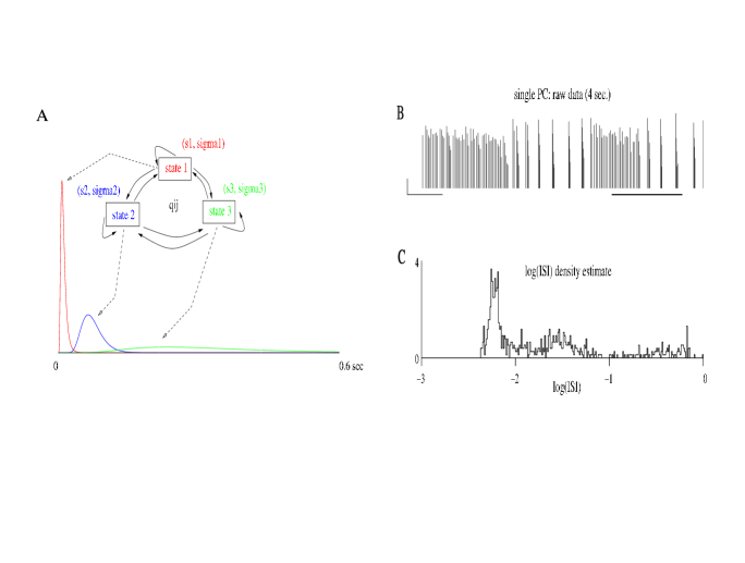
Figure 1: Model for the ISI density compared to a real spike train. A, ISI density model: a Hidden Markov Model with three states. Every state is a log-normal density with 2 parameters: a scale parameter s (in seconds) and a shape parameter (dimensionless) $\sigma$: (0.01 sec., 0.5) state 1, (0.07 sec., 0.3) state 2, (0.3 sec., 0.5) state 3. B, spontaneous activity of a single PC in presence of bath-applied DHPG (40 $\mu M$) in loose cell-attached. Normalized peak amplitudes of the detected events are shown (duration: 4 seconds). The thick horizontal bar on the right indicates the part of the train shown in Fig. 2B. Horizontal scale bar: 0.5 sec. Vertical scale bar: 5 (in units of noise SD). C, $\log_{10}\left(isi\right)$ histogram of the same spike train as in A (1 minute, 763 spikes). Bin width: 0.01.

Fig. 1B shows 4 seconds of a typical spike train of a PC in DHPG. Note the presence of bursts of spikes of dramatically decreasing amplitudes. The ISI histogram of this train (763 spikes, 1 minute of recording) is plotted in Fig. 1C. The multi-modal character of this histogram is unambiguous. This type of activity (usually on the order of one minute) alternates with silent periods with a similar duration of one minute.

3.2 A 3-state Hidden Markov Model fits well empirical inter-spike interval densities

We used our MCMC algorithm without the REM (see Methods) to fit our 3-state HMM parameters, as well as the amplitude parameters (see sec. 3.3, for the fit of amplitude parameters), from this single unit spike train. In this section, where no spike-sorting is performed, our algorithm only fits the model parameters of the single cell recorded and attributes one of the three HMM states to each spike in this single unit spike train. Fig. 2A shows the evolution of the dimensionless shape parameters $\sigma_{1}$ (red), $\sigma_{2}$ (blue), $\sigma_{3}$ (green) during a 1000-MC steps run. Only the first 500 MC steps are displayed, but there was absolutely no change in the evolution of these parameters between steps 500 and 1000. All other parameters (scale parameters $\mathrm{s_{1}}$, $\mathrm{s_{2}}$, $\mathrm{s_{3}}$ and transition parameters $\mathrm{q_{ij}}$) had similar evolutions. Note that the algorithm reaches equilibrium very fast (after about 20 MC steps). The average values of $\mathrm{s_{1}}$, $\mathrm{s_{2}}$, $\mathrm{s_{3}}$ (autocorrelation corrected SDs given in parenthesis, see Methods sec. 2.2.4) computed on the last 200 iterations were 6 (0.08) ms, 28 (1) ms, 392 (22) ms respectively. These scale values are to be compared to the location of the 3 ISI histogram’s modes described in what follows. The average values of $\sigma_{1}$, $\sigma_{2}$, $\sigma_{3}$ (autocorrelation corrected SDs given in parenthesis, see Methods sec. 2.2.4) were 0.246 (0.01), 0.538 (0.026), 0.494 (0.041) respectively.

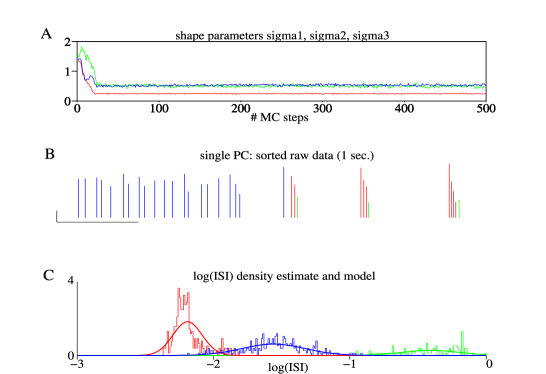
Figure 2: Sorting ISI modes in a cell engaged in complex bursting behavior. MCMC output after a 1000-MC step run on the spike train shown in Fig. 1. A, evolution of the shape parameters $\sigma$₁, $\sigma$₂, $\sigma$₃ during this 1000-step run. Only the first 500 MC steps are shown (same color code as in Fig. 1). B, spike label analysis of the episode indicated by the thick horizontal bar of Fig. 1B. Each spike is colored according to its most probable HMM state determined by the algorithm (same color code as in Fig. 1). Horizontal scale bar: 0.2 sec. Vertical scale bar: 5 (in units of noise SD). C, $\log_{10}\left(isi\right)$ histogram of each state for the most probable configuration (same color code as in Fig. 1). Note that each state corresponds to one mode of the histogram of Fig. 1C. The 3 model densities whose parameters have been set at their average values computed on the last 200 iterations are superimposed on the histogram.

Fig. 2B shows part of the spike train of Fig. 1B. At each step the algorithm attributes one of the 3 possible states to each spike. The configuration (i.e. the labeling of each spike with a neuron state’s number) shown in Fig. 2B is the most frequent one computed over the last 200 steps of the 1000-step run displayed in A. We use the same color code as in Fig 1A. As expected, spikes in bursts are attributed by the algorithm to a short state (red) label, except for the last spike of the burst which is followed by a long ISI and is thus attributed to a long state (green) label. Spikes occurring during regular spiking and separated by intermediate ISIs are attributed the intermediate state (blue) label.

In Fig. 2C, the ISI histogram of this spike train has been subdivided and colored according to the state of the neuron: all ISIs generated when the neuron was in the short state (resp. intermediate, long) are plotted in red (resp. blue, green), as expected. Superimposed on this histogram are the 3 model ISI densities whose parameters have been set to their average values computed on the last 200 MC steps and given above. The reader sees that the initial ISI histogram displayed in Fig. 1C is reasonably well fitted by this mixture of three log-normal densities (the most striking deviation between the actual data and the fit being observed for the short state). Moreover, besides its ability to describe a multi-modal ISI histogram, the HMM can also account for the dependence between successive ISIs through its transition matrix. In our case, a long state is always followed by a short state, as shown more quantitatively in sec. A.2.1 of the Appendix.

These results show that the model we propose can satisfyingly, but not perfectly, account for the discharge considered here. In Fig. 3 we provide the interested reader with a goodness-of-fit test based on Kolmogorov-Smirnov plots. It shows that this spike train clearly supports this 3 log-Normal state HMM when compared to models with 2 and 1 state(s).

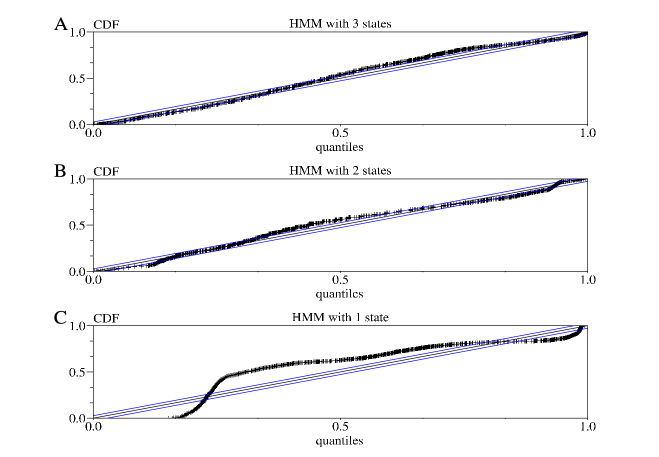
Figure 3: Kolmogorov-Smirnov (K-S) plots of the Hidden Markov Models fits to the PC spike train shown in Fig. 1 and 2. A, HMM with 3 log-normal states. B, HMM with 2 log-normal states. C, HMM with 1 log-normal state. In A, B and C, the solid 45-degree line represents exact agreement between the model and the data. The 45-degree lines on both sides are the 95% confidence bounds for exact agreement between the model and experimental data based on the Kolmogorov-Smirnov statistics. Although not perfect, a HMM with 3 states obviously fits better the PC spike train than a HMM with 2 or 1 state(s). CDF stands for Cumulative Distribution Function. For details about Kolmogorov-Smirnov tests, see BrownEtAl_2001 .

Between two periods of silence, a period of PC activity in DHPG always evolves from a tonic firing at about 15 Hz (second mode of the ISI histogram) to a bursty firing with 150 Hz-bursts (first mode of the ISI histogram) separated by intervals of several hundreds of ms (third mode of the ISI histogram). This is well illustrated on Fig. 1B which represents a transition from this tonic to bursty firing. The minute of activity shown in Fig. 1, 2 and 4 depicts perfectly this evolution. However, in the case where only the short bursts are recorded, only 2 modes are prevailing (the short and the long ones). Such a case is obvious in the multi-unit data analyzed in section 3.4.

3.3 Spike amplitudes relax exponentially with respect to inter-spike interval duration

The second part of our data generation model concerns the dependence of spike amplitude upon the time elapsed since the last spike of the same neuron. We also checked whether our PC spike trains supported this hypothesis. We use here the same data set as in section 3.2. In Fig. 4A, the normalized peak amplitude of each detected spike is plotted against the ISI that preceded it. Recall that this single unit data were obtained with one recording site, so that only one peak amplitude per spike is to be considered. The exponential relaxation with parameter values determined by our algorithm is superimposed on the data points. The reader is referred to section 2.2 where this exponential model is presented. For this particular train, parameter values are (SDs given in parenthesis): $P=20.3\,(0.03)$, $\delta=0.617\,(0.007)$, $1/\lambda=17\,(0.4)\,ms$. $P$ is given in noise SD and $\delta$ is dimensionless.

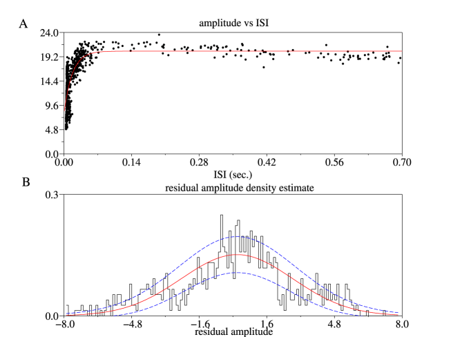
Figure 4: Model for the spike amplitude dynamics. A, Events normalized peak amplitudes plotted with respect to the ISI preceding the event (dots). The fitted exponential relaxation is superimposed (solid line). Ordinates in units of noise SD. B, Histogram of the residual amplitudes. The Gaussian fit is superimposed (solid line). The two dashed lines are one SD away from the expected histogram.

Several issues now must be addressed with respect to the peak amplitude variance of the neurons we measured. First, the variability of spikes amplitudes at short ISIs (around 5 ms) seems to be larger than those at intermediate or long ISIs. This “over-variability” is mainly a visual effect for a narrow range of short ISIs is significantly more represented. This over-represented population necessarily samples the Gaussian distribution more thoroughly. Second, a group of points with an abscissa around 10 ms as well as points with abscissa greater than 400 ms are clearly below the exponential fit, while points with abscissa in 50-400 ms range are slightly above it. Third, these two significant deviations compensate each other. This is shown by the histogram of the residual amplitudes displayed in Fig. 4B to which a fitted Gaussian density with an SD equal to 2.64 is superimposed. The SD of the residual amplitude histogram has been both added to and subtracted from the fitting Gaussian curve (upper and lower dashed line respectively). One sees that an exponential relaxation of amplitudes looks like a good first approximation of the actual amplitude dynamics. One sees as well that our third hypothesis is only an approximation, for our residual here exhibit a larger variability (an SD of 2.64) than the one expected from the measured background noise (SD of 1). In particular, these data exhibit a slight but clear decrease of amplitude with long ISIs, whereas our model keeps a fixed, maximal amplitude for these ISIs.

3.4 Multi-unit data sorted by our algorithm

3.4.1 Multi-unit data and reference neuron

We performed multi-unit recordings of spontaneously active PCs in the presence of DHPG using a multi-site electrode that we positioned along the PC layer. A glass micropipette was placed in loose cell-attached next to site 3 of the multi-site electrode in order to independently monitor the activity of one of the PCs from the recorded population. Such data were kept only if the glass micropipette unambiguously recorded the activity of a single cell with an excellent signal-to-noise ratio. This cell is called “reference cell” and the detected events of these recordings serve as “reference events” to which the output of our algorithm is compared. In what follows, we show the performance of our spike-sorting algorithm on a representative example of these recordings (58 seconds, 2739 events detected). Each detected event is described by its time of occurrence and the 4 peak amplitudes on the 4 recording sites after noise whitening.

3.4.2 The reference neuron is reliably labeled as unit 1

The following results were obtained after a 1000-MC steps with the REM and the following “inverse temperatures”: $\beta=1,\,0.975,\,0.95,\,0.925,\,0.9,\,0.875,\,0.87$ followed by 1000 steps with $\beta=1$ only. This required about 33 minutes on a 3 GHz PC (Pentium IV) running Linux. Plots of energy evolution and parameters evolution showed that all parameters had reached their equilibrium value after roughly 500 MC steps (not shown). We computed the average value of each model parameter using the last 200 MC steps. We also forced the soft classification produced by our algorithm into the most likely classification using the last 200 MC steps PouzatEtAl_2004 .

Fig. 5A shows two separate periods of 2 seconds from these data (peak amplitudes of the detected events after noise whitening, see Methods). Each row corresponds to one recording site of the Michigan probe (site 1 to site 4 from top to bottom), as depicted on the left. Each event is colored according to its most probable neuron of origin: neuron 1 in black, neuron 2 in deep blue, neuron 3 in green, neuron 4 in light blue, neuron 5 in red, neuron 6 in brown. A raster plot of the reference events is displayed in the upper part of the site 3 panel. From these plots, it is obvious that the black unit (unit 1) reconstructed by our algorithm corresponds to the reference cell (see details below). Note that the event amplitudes of this cell are strongly reduced within the bursts so that they become similar to those produced by unit 5 (red). This of course makes the separation between these 2 units really difficult.

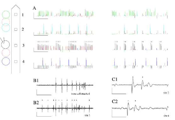
Figure 5: Spike sorting on a mixture of several PC spike trains simultaneously recorded (1). A,  spontaneous activity of PCs with bath-applied DHPG recorded on the first 4 sites of the electrode. Two separate periods of 2 seconds taken from the same minute of recording are shown (peak amplitudes of the detected events after noise whitening). Each event is colored according to the label determined by our algorithm. These labels are the most probable ones over the last 200 steps of a 1000-step run. An independent recording was performed next to site 3 by a patch-clamp pipette in loose cell attached. A raster plot of this reference neuron’s activity is displayed in the upper part of the panel of site 3. A scheme of the first 4 sites of the electrode as well as the recorded PCs with the positioned extracellular glass pipette are drawn on the left. Horizontal scale bar: 0.5 sec. Vertical scale bar: 10 (in units of noise SD). B1: raw data recorded by the extracellular glass pipette in loose cell attached, showing a typical burst. Horizontal scale bar: 100 ms. Vertical scale bar: 0.5 mV. B2, corresponding raw data recorded by site 3 of the multi-site electrode, showing the detected burst. Crosses are drawn on top of the detected events (the same holds for C1 and C2). Horizontal scale bar: 100 ms. Vertical scale bar: 0.25 mV. C1, raw data recorded by site 2 of the multi-site electrode, showing a typical triplet. Horizontal scale bar: 10 ms. Vertical scale bar: 0.5 mV. C2, raw data recorded by site 4 of the multi-site electrode, showing a typical triplet (detected as doublet). Horizontal scale bar: 10 ms. Vertical scale bar: 0.25 mV.

Raw data from site 3 are displayed in Fig. 5B2 (crosses are drawn on top of the detected events), showing one of the bursts of unit 1 as well as a “background” cell (for example, the first three detected events on this panel come from this background cell). As the spike amplitude decreases within the burst of unit 1, these spikes end up being of the same size as this background cell. The latter is labeled as unit 5 by our algorithm (red on panel A). The corresponding raw data recorded by the independent micropipette are displayed in Fig. 5B1. Note the huge signal amplitude, as well as the decreasing spike amplitudes along the burst. The activity recorded by the micropipette unambiguously comes from a unique PC. These two panels B1 and B2 allow a direct comparison of the signal received by site 3 of the microelectrode to the one received by the pipette: the latter records the burst seen on panel B2 only, and not the background cell. They also illustrate the fact that not all events of the reference cell are detected on site 3: the very last spikes of each burst fired by the reference cell are much smaller and below our detection threshold. For that reason, among the 766 reference events detected on the micropipette trace during this minute of data, 641 are detected on the trace of site 3. Among these 641 events, 629 are attributed to unit 1 by our algorithm (98,1%). Overall, 637 events are attributed to unit 1 so that 8 unit 1 events are not reference events (false positives, 1.3%). The 12 reference events not labeled as unit 1 are labeled as unit 5 (red). For comparison, a classical Gaussian mixture model (GMM) fitted with the Expectation-Maximization (EM) algorithm (Pouzat et al., 2002), attributes only 542 reference events to unit 1 (84.5%), the 99 remaining ones being attributed to unit 5. To illustrate this comparison, Fig. 6 displays the Wilson plots, where the amplitude on site 4 is plotted against its amplitude on site 3, after running the EM and the MCMC algorithms separately: the Gaussian mixture model partially truncates the elongated cluster of our reference neuron, whereas our elaborated and more realistic model does not. This excellent performance of our algorithm in such a difficult situation shows how powerful it is to incorporate the temporal information into the spike-sorting procedure through an appropriate model for the neuronal discharge statistics.

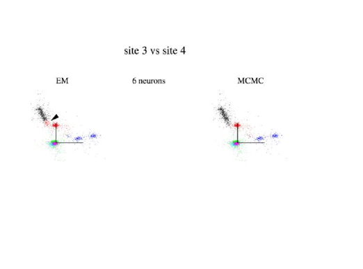
Figure 6: Comparison between the sorting performed by the Expectation Maximization (EM) algorithm and the MCMC algorithm. Wilson plots (peak amplitudes of site 3 versus site 4) after sorting based on a classic GMM(using the EM algorithm, left) and on our new data generation model (using an MCMC algorithm, right) with 6 neurons. The analysis performed with the MCMC algorithm for this number of neurons is given in details in the article. The GMM fails to group all the points of the reference neuron (black cluster), so that the cluster is partially cut and attributed to the red one (arrow head): the GMM attributes 84.5% of the reference events to the reference neuron (versus 98,1% for the MCMC algorithm, see sec. 3.4.2). This illustrates how inappropriate the GMM is with non-Gaussian, elongated clusters. In such cases, implementing both the discharge statistics of the neuron and its amplitude dynamics in the spike sorting method very satisfyingly solves the problem.

Similar results were found in five other data sets of bursting PCs, where the MCMC algorithm with the present HMM model outperformed the EM algorithm. In three of these data sets, an extra pipette separately recorded a reference cell: in these cases, our algorithm was able to rebuild more than 96% of the bursts of the reference cells, with less than 3% false positives.

3.4.3 Unit 2 and unit 4 give rise to pairs of separated clusters on Wilson plots

Two other units deserve being examined. Unit 2 (deep blue, site 4) and unit 4 (light blue, site 2) produce doublets of spikes of very different amplitudes. Nevertheless, in both cases, these events are recognized as coming from the same cell. The corresponding raw data recorded on site 2 and site 4 are displayed in Fig. 5C1 and C2 respectively. These two panels show one typical burst of each cell: in both cases, these bursts are in fact triplets of spikes. In the case of site 4, the third spike of each burst remains below detection threshold, so that only a doublet is detected (crosses on top of the detected events). All these doublets are correctly identified as coming from unit 2 (deep blue, Fig. 5A). In the case of site 2, the third spike of each burst is detected, but is wrongly attributed to unit 6 (brown, Fig. 5A), instead of being attributed to unit 4, like the first two spikes of the triplet (light blue, Fig. 5A). This misclassification is essentially due to the fact that our model of spike waveform dynamics is not accurate enough for the data from this neuron, as discussed in sec. A.2.2 and Fig. 8 in Appendix. This misclassification should moreover serve as a warning against a blind use of our algorithm which would consist in taking the output for granted without checking its relevance at all. The plots displayed in Fig. 5A and Fig 7A,B should be drawn after each run in order to assess the quality of the sorting. In particular the ISI histograms of the sorted neurons must show a clear refractory period and an overall shape that is similar to ISI histograms of single cell recordings that can be obtained separately.

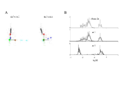
Figure 7: Spike sorting on a mixture of several PC spike trains simultaneously recorded (2). A, Wilson plots (peak amplitudes of site 3 against site 2 and site 4 respectively) showing the whole recorded sample (2739 events, 58 seconds). Each event is colored according to the most probable label determined by our algorithm (same colors as in Fig. 5A). The reference unit is in black. Note the 2 pairs of separate clusters: in light blue (site 2) and deep blue (site 4) on the lefthand and righthand plots respectively. Note also the very elongated cluster on both plots in black (site 3). On each plot the scale bars meet at amplitude (0,0) and are of size 10 (in units of noise SD). B, $\log_{10}(isi)$ histograms of units 1 (black cluster in A) and 2 (deep blue cluster in A). Their 3 respective model densities whose parameters have been set at their average values computed on the last 200 iterations are superimposed on their respective histograms. The $\log_{10}(isi)$ histogram of the reference unit is also shown and to be compared to unit 1 histogram.

Fig. 7A shows Wilson plots of the data with the same color code as in Fig. 5A. Only two plots out of six are displayed. As in Fig 5A, unit 1 that corresponds to the reference cell is in black. Note the elongation of this cluster. Note also the 2 distinct, well separated clusters of unit 4 (light blue) on the left hand plot.

3.4.4 Empirical and modeled ISI densities

We finally display the ISI histograms of units 1 and 2, as well as the one of the reference events detected on site 3 of the multi-site electrode (Fig. 7B). The similarity between the histogram of unit 1 and that of the reference cell is another illustration of the 98% performance of the algorithm on this unit. Note the 3 modes of this histogram. The 3 ISI model densities of unit 1 and unit 2 with parameters set at their average values computed over the last 200 MC steps are superimposed on their respective ISI histograms. For unit 1, the 3 scale values are (autocorrelation corrected SDs given in parenthesis) {13 (1.6) ms, 35 (1.5) ms, 314 (5) ms}, whereas the 3 shape values are {0.395 (0.059), 0.262 (0.035), 0.194 (0.013)}. The scale values approximately locate the different modes of the histogram. For unit 2, we have {5 (0.06) ms, 92 (42) ms, 374 (12) ms) and {0.148 (0.009), 1.62 (0.479),0.224  (0.028)}. Only 20 events of unit 2 (out of 301) are found to be in state 2. They correspond to the few bins between the 2 modes of this histogram. As pointed out in the next to last paragraph of section 3.2, this unit only fires 150-Hz bursts during this minute of recording. The more tonic firing that always occurs before was already over for this unit by the time the recording started. This is why almost no intermediate ISI is to be seen in this case. Each model density being of course normalized by the proportion of events in each state for a given unit, the curve corresponding to state 2 is almost null everywhere and does not appear on the plot. This shows that, although the ISI histogram of unit 2 is essentially bimodal, the behavior of the algorithm is not altered at all. Our 3-state HMM can well accommodate any bi- or unimodal ISI histogram. Like in section 3.2, this shows how well the HMM accounts for the discharge statistics of bursting cells that have tri- or bimodal ISI histograms.

4 Discussion

We have shown here how the spike-sorting algorithm we recently proposed PouzatEtAl_2004 , Pouzat_2005 , modified for multi-state neurons, performs on real, challenging data. In this data set, i.e. PCs in presence of DHPG, the recorded cells were firing bursts of spikes whose amplitudes were strongly reduced, producing distinct, well separated clusters in the Wilson plots (deep blue and light blue clusters in Fig. 7), as well as very elongated ones (black cluster in Fig. 7). To check the performance of the algorithm, the activity of one of the recorded PCs was independently and simultaneously monitored by a loose cell-attached glass micropipette and served as reference spike train. We showed that our algorithm did properly classify more than 98% of this reference spike train, despite the obvious decrease of spike amplitudes (Fig. 5A,B1,B2 & 7A) and the tri-modal ISI histogram (Fig. 7B). We showed as well that it did associate the pairs of distinct clusters mentioned above, obviously produced by a single neuron. In such situations, existing methods require that the experimentalist a posteriori groups by himself the spikes that have been wrongly assigned to different neurons due to their changing amplitudes. None of them can automatically give such an output on these data.

The excellent performance of our method relies on its ability to take into account the information provided by the occurrence time of the spikes, as well as their amplitude dynamics. To our knowledge, this is the only method that makes use of these real spike trains properties. It is moreover built on a proper probability model for data generation which, in that case, implies that convergence proofs of the algorithm do exist PouzatEtAl_2004 , Pouzat_2005 . Our MCMC based approach provides as well meaningful confidence intervals on the model parameters and on the spike labels, a feature which should not be overlooked.

We have also illustrated here the flexibility of the MCMC framework. In our previous reports PouzatEtAl_2004 , Pouzat_2005 we used a simpler model for the discharge dynamics of the neurons: a single log-normal density modeled the neurons ISI histograms. Here we first showed that a multi-state HMM discharge model CamprouxEtAl_1996 , GucluBolanowski_2004 was well supported by our single unit data (see sec. 3.2). We then included this model in our spike-sorting algorithm and ran it on the multi-unit data. The message is that once one knows how to write down an MCMC algorithm for a “reduced” problem like generating the parameters of the three states discharge model of a single neuron, it is straightforward to incorporate it into the full spike-sorting algorithm. Therefore if the experimentalist, based on single unit data (obtained for instance with patch or sharp electrode recordings) thinks that another discharge model would be better, the spike-sorting algorithm does not need to be rewritten from scratch, only a sub-part of it needs to be modified. We nevertheless think that the data generation model presented here will turn out to be a good compromise between accuracy of the description of real data and ease and speed of implementation. We did not seek to relate each individual state of our HMM to any particular biophysical event or set of events. This model has to be considered as a statistical, descriptive tool that captures the key features of the observed neuronal bursty firing. It is not limited to bursty firings though: in our model, 3 states are available to describe the empirical ISI density, but of course, one or two of these states can be unused for a unit that has a uni- or bimodal ISI histogram (see unit 2 in section 3.4.4). Therefore, our model can account for uni- and bimodal ISI histograms as well, of course better than a Poisson model would. In addition, the number of states is not fixed at all and the experimentalist can choose it himself as an input to the algorithm, a priori and for each neuron.

PCs are known to tonically fire action potentials as well as bursts of spikes spontaneously in slices at 35 °C, even when fast synaptic inputs are completely blocked WomackKhodakhah_2002 . This spontaneous activity is preserved at room temperature but bursts of spikes are less frequent. We facilitated the spontaneous bursting behavior of PCs by adding DHPG to the bathing solution NetzebandEtAl_1997 . This enables us to get multiunit data in which most of the cells fire bursts of spikes of decreasing amplitudes and helps demonstrate the ability of our spike-sorting method to automatically isolate these bursts.

For now the method is not fully automatic in the sense that it requires the user to choose the number of neurons a priori and give it as an input to the algorithm. As discussed in PouzatEtAl_2004 , the general frame of the method provides a way to reliably compare models with different numbers of neurons. This still ongoing work will be reported in a near future.

Appendix A Appendix

A.1 Methods

A.1.1 A formal presentation of the HMM

We extend here our previous model PouzatEtAl_2004 , Pouzat_2005 by introducing multiple discharge states, $D=d$, with $d\in\{1,\ldots,N_{ds}\}$, for each neuron (in this paper we set the number of states $N_{ds}$ at 3). The goal is to be able to describe at the same time multi-modal ISI densities (i.e., densities with several peaks) and dependence between successive ISIs similar to what goes on during a burst, where (single) “silent periods” (long ISIs) are followed by many short ISIs (see sec. A.2.1 for an example). Following CamprouxEtAl_1996 we assume that successive ISI are independent conditioned on the neuron’s discharge state, $d$. After the emission of each spike (i.e., the generation of each ISI) the neuron can change its discharge state or keep the same. The inter discharge state dynamics is given by a Markov matrix, $Q=(q_{ij})$. We moreover assume that the ISI distribution of each state is log-normal. In other words we assume that the neuron after its $m$th spike is in state $d$ and that the ISI between this spike and the next one is distributed as:

$$ISI\mid d\sim\textrm{log-normal}(s_{d},\sigma_{d})$$ (7)

Eq. 7 should be read as:

$$\pi_{isi}(ISI=isi\mid S=s_{d},\Sigma=\sigma_{d})=\frac{1}{isi\cdot\sigma_{d}\cdot\sqrt{2\pi}}\cdot\exp\Big{(}-\frac{1}{2}\big{(}\frac{\log(isi)-log(s_{d})}{\sigma_{d}}\big{)}^{2}\Big{)}$$ (8)

where $S$ is a scale parameter (measured in seconds) and $\Sigma$ is a shape parameter (dimensionless). These random variables do depend on the value taken by the random variable $D$. After the ISI has been generated, the neuron can “move” to any of its $N_{ds}$ states according to a probabilistic dynamics described by:

$$\textrm{P}(D^{(m+1)}=j\mid D^{(m)}=i)=q_{ij}$$ (9)

You see therefore that if we work with a neuron with 3 discharge states we have 12 independent ISI parameters to estimates: 2 pairs $(s,\sigma)$ per state and $N_{ds}\cdot(N_{ds}-1)$ state transition parameters (do not forget that matrix $(q_{ij})$ is stochastic and therefore its rows sum to 1).

A.1.2 Generating a new state in the Markov chain

In this section, we use $Y$ to designate the data. At step $t$, state $\left[\theta^{\left(t\right)},C^{\left(t\right)}\right]$ is drawn from state $\left[\theta^{\left(t-1\right)},C^{\left(t-1\right)}\right]$ by successively drawing each model parameter and each spike label and spike state according to the procedures described below. To simplify notations we omit the step index $(t)$ of the generated state. We note $C_{-i}$ the configuration specifying the labels and neuron states for all the spikes except spike number $i$. Similarly we note $\theta_{-a}$ the vector of all model parameters except parameter $a$. Each parameter $a$ has a uniform prior on a defined segment $\left[a_{min},a_{max}\right]$ relevant for this parameter PouzatEtAl_2004 . A step of our algorithm is performed once all spike labels and states, as well as all model parameters have drawn as specified below. This defines the new state in the Markov chain.

Labels and neuron states

For each spike $i$ of the spike train, a label $l_{i}\in\left\{1,...,K\right\}$ and a neuron state $m_{i}\in\left\{1,2,3\right\}$ are drawn from their posterior conditional density:

$$l_{i},m_{i}\mid Y,\theta,C_{-i}\sim\frac{\pi_{post}(l_{i},m_{i}\mid Y,\theta,C_{-i})}{\sum_{l_{j},m_{j}}\pi_{post}(l_{j},m_{j}\mid Y,\theta,C_{-i})}$$ (10)

Amplitude parameters

For each neuron $q$, the amplitude parameters ($P_{q,1},P_{q,2},P_{q,3},P_{q,4},\delta_{q},\lambda_{q}$) are drawn with a Metropolis-Hastings step, using piecewise linear approximations of their respective posterior conditional densities as proposals PouzatEtAl_2004 . Let us take the case of $\lambda_{q}$, for example, to illustrate the procedure. Let $\pi_{post}\left(\lambda_{q}\mid Y,\theta_{-\lambda_{q}},C\right)$ be its posterior conditional density and $\tilde{\pi}_{approx}\left(\lambda_{q}\mid Y,\theta_{-\lambda_{q}},C\right)$ be its piecewise linear approximation. Let $\lambda$ be the current value of $\lambda_{q}$.

First, $\tilde{\lambda}$ is drawn from the proposal density:

$$\tilde{\lambda}\mid Y,\theta_{-\lambda_{q}},C\sim\tilde{\pi}_{approx}\left(\lambda_{q}\mid Y,\theta_{-\lambda_{q}},C\right)$$ (11)

Then, this value $\tilde{\lambda}$ is accepted with probability $A$ equal to:

$$A=\min\left(1,\frac{\pi_{post}\left(\tilde{\lambda}\mid Y,\theta_{-\lambda_{q}},C\right)\cdot\tilde{\pi}_{approx}\left(\lambda\mid Y,\theta_{-\lambda_{q}},C\right)}{\pi_{post}\left(\lambda\mid Y,\theta_{-\lambda_{q}},C\right)\cdot\tilde{\pi}_{approx}\left(\tilde{\lambda}\mid Y,\theta_{-\lambda_{q}},C\right)}\right)$$ (12)

If $\tilde{\lambda}$ is accepted, then $\lambda\rightarrow\tilde{\lambda}$.

Else $\lambda\rightarrow\lambda$

Log-Normal parameters

scale parameters

For each neuron $q$ and each neuron state $r$ ($r\in\left\{1,2,3\right\}$) of neuron $q$, the scale parameter of the log-Normal density is noted $s_{q}^{r}$.

First $u$ is drawn from PouzatEtAl_2004 :

$$u\mid Y,\theta_{-s_{q}^{r}},C\sim Norm\left(\overline{\log i_{q}},\frac{\left(\sigma_{q}^{r}\right)^{2}}{n_{q}}\right)$$ (13)

where $n_{q}$ is the number of ISI of neuron $q$, $\sigma_{q}^{r}$ is the shape parameter of neuron $q$ in neuron state $r$, and $\overline{\log i_{q}}=\frac{1}{n_{q}}\sum_{j=1}^{n_{q}}\log i_{q,j}$, $i_{q,j}$ being the ISI index $j$ of neuron $q$.

Then, if $s=\exp\left(u\right)\in\left[s_{min},s_{max}\right]$, we set $s_{q}^{r}=s$.

Else we draw another $u$.

shape parameters

For each neuron $q$ and each neuron state $r$ ($r\in\left\{1,2,3\right\}$) of neuron $q$, the shape parameter of the log-Normal density is noted $\sigma_{q}^{r}$.

First $u$ is drawn from PouzatEtAl_2004 :

$$u\mid Y,\theta_{-\sigma_{q}^{r}},C\sim Gamma\left(\frac{n_{q}}{2}-1,\frac{n_{q}}{2}\left(\overline{\log i_{q}}-\log s_{q}^{r}\right)^{2}\right)$$ (14)

with the same notations as for the scale parameters.

Then, if $\sigma_{min}\leq\sqrt{1/u}\leq\sigma_{max}$, we set $\sigma_{q}^{r}=\sqrt{1/u}$.

Else we draw another $u$.

Transition parameters

For each neuron $q$, the transition parameters between the 3 HMM neuron states form a 9 by 9 matrix whose 3 rows are drawn successively.

Let $m=(m_{1},...,m_{N})$ be the spike train configuration of a neuron $q$, where $m_{k}$ is the neuron state of spike $k$ of this neuron. Let $\mathrm{n_{ij}}$ be the number of spikes of this neuron which are in state $m_{j}$ following a spike of this neuron in state $m_{i}$. The row number i of the transition matrix is then drawn from the Dirichlet distribution $\mathrm{\mathcal{D}_{3}}(1+n_{i1},1+n_{i2},1+n_{i3})$ RobertCasella_1999 .

A.1.3 Implementation details

Codes were written in C. We used the free softwares Scilab and R to generate output plots as well as the graphical user interface. The GNU Scientific Library (GSL) was used for vector and matrix manipulation routines and (pseudo-)random number generators. More specifically, the GSL implementation of the Mersenne Twister of Matsumoto and Nishimura MatsumotoNishimura_1998 was used to generate random variates. Codes were compiled with the intel icc compiler and run on a PC (Pentium IV 3 GHz) running Linux.

A.2 Supplementary analysis

A.2.1 Dependence between successive ISIs in the single unit spike train.

The transition matrix $\left(\mathrm{q_{ij}}\right)$ of the most probable configuration (i.e the attribution of a neuron state to each spike) of the single unit spike strain shown in Fig. 1 and 2 is given below. The lowest and largest values taken by each transition element over the last 200 MC-steps are given in square brackets. The neuron state numbers (i.e here, the row and column numbers) are those of Fig. 1 and 2, that is: states 1, 2 and 3 for the short, intermediate and long ISIs respectively. The dependence between ISIs is obvious: a long ISI is always followed by a short ISI ($\mathrm{\mathrm{q_{31}=1}}$), a short ISI is either followed by another short ISI (within a burst), or by a long ISI almost exclusively ($\mathrm{q_{11}=0.69}$ and $\mathrm{q_{13}=0.3}$). This is in agreement with the existence of bursts separated by longer intervals. This may be related to the refractory period after high frequency discharge in burst. If successive ISIs were independent, rows would be identical, each column being equal to the proportion of the state.

	state 1	state 2	state 3
state 1	0.69 [0.62; 0.76]	0.01 [0; 0.03]	0.3 [0.23; 0.38]
state 2	0.02 [0; 0.06]	0.98 [0.94; 0.99]	0 [0; 0.03]
state 3	1 [0.91; 1]	0 [0; 0.08]	0 [0; 0.04]

A.2.2 Why are the third spikes of unit 4 triplets wrongly attributed to unit 6?

First of all, the event amplitudes of unit 6 are very similar to the amplitudes of the third spikes of unit 4 triplets, which considerably complicates the separation between these two units. In fact, the likelihood of the data is significantly smaller when these spikes are rightly labeled as unit 4 than when they are labeled as unit 6, which explains the output of the algorithm. This is due to the fact that our model of waveform dynamics is not sufficiently supported by data from unit 4, so that, with this model, its third spikes in bursts are more likely to come from unit 6, whose events are of similar amplitude, as shown in Fig. 5A, site 2. This point is described in detail in Fig. 8. Second, as illustrated on the raw data of site 2 (Fig. 5C1), the third spikes of these bursts have an overall different waveform (note that the valley preceding the peak almost disappears). In this case, we are not dealing with a simple homothetic scaling of the waveform. That is why we also ran the algorithm using 3 points per site and per event, instead of the peak amplitude only. This was not sufficient to correctly label these spikes as unit 4. In fact, using 3 points per site and per event instead of the peak amplitude did not change the output of the algorithm in this case. Third, the spikes at stake here are really small spikes that might even not be detected in other circumstances. Whatever the spike-sorting method, small events are always less reliably labeled and the experimentalist has to leave them out and keep the unambiguous ones. We certainly do not claim that our method can overcome this limit. In this case, any reasonable experimentalist who has been dealing with spike-sorting would not take into account these events.

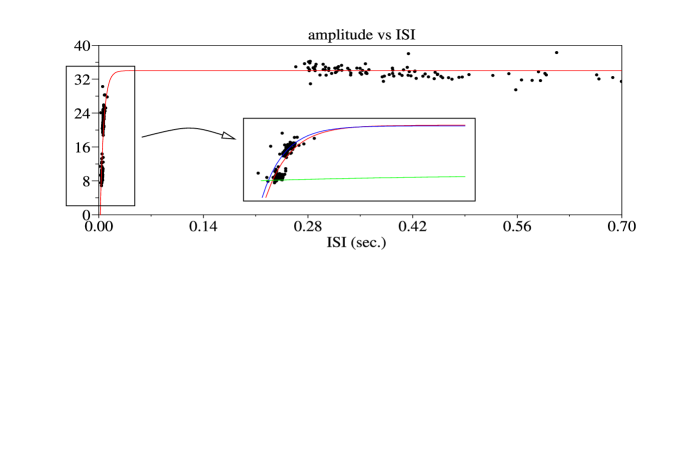
Figure 8: Amplitude dynamics of spikes within the triplets of unit 4. The third spikes of unit 4 triplets (labeled as unit 6 by our algorithm) and the spikes labeled as unit 4 are pooled together to form the real spike train of unit 4. The peak amplitudes (after noise whitening) of these spikes are plotted with respect to the ISI preceding the spike (black dots). The fitted exponential relaxation is superimposed (red solid line). Ordinates in units of noise SD. The inset shows an expanded version of the left hand part of the plot and shows that the model does not perfectly account for the waveform dynamics of this unit. This leads to a relatively low likelihood of this spike train, whereas removing the third spikes (lowest group of points) of each triplet from unit 4 and attributing them to unit 6 allows a better global fit (blue solid line for unit 4 and green solid line for unit 6). The likelihood of the whole is lower in the latter case, i.e. when the third spikes of unit 4 triplets are labeled as unit 6. This explains why the algorithm fails to fully reconstruct unit 4 triplets.

References

- [1] Baker SN, Philbin N, Spinks R, Pinches EM, Wolpert DM, MacManus DG, Pauluis Q, Lemon RN. Multiple single unit recording in the cortex of monkeys using independently moveable microelectrodes. J Neurosci Methods, 1999; 94:5-17.
- [2] Brown EN, Barbieri R, Ventura V, Kass RE, Frank LM. The Time-Rescaling Theorem and Its Application to Neural Spike Train Data Analysis. Neural Comp, 2001; 14:325-46.
- [3] Brown EN, Kass, RE and Mitra PP. Multiple neural spike train analysis: state-of-the-art and future challenges. Nature Neurosci, 2004; 5:456-61.
- [4] Buzsaki G. Large scale recording of neuronal ensembles. Nature Neurosci, 2004; 5:446-51.
- [5] Camproux AC, Saunier F, Chouvet G, Thalabard JC, Thomas G. A Hidden Markov Model Approach to Neuron Firing Patterns. Biophys J, 1996; 71:2404-12.
- [6] Csicsavari J, Henze DA, Jamieson B, Harris KD, Sirota A, Bartho P, Wise KD, Buzsaki G. Massively Parallel Recording of Unit and Local Field Potentials With Silicon-Based Electrodes. J Neurophysiol, 2003; 90:1314-23.
- [7] Drake KL, Wise KD, Farraye J, Anderson DJ, and Bement SL. Performance of planar multisite microprobes in recording extracellular single-unit intracortical activity. IEEE Trans Biomed Eng, 1988; 35:719-32.
- [8] Egert U, Heck, D, Aertsen A. Two-dimensional monitoring of spiking networks in acute brain slices. Exp Brain Res, 2002; 142:268-274.
- [9] Fee MS, Mitra PP, Kleinfeld D, Automatic sorting of multiple-unit neuronal signals in the presence of anisotropic and non-Gaussian variability. J Neurosci Methods, 1996a; 69:175-188.
- [10] Fee MS, Mitra PP, Kleinfeld D. Variability of extracellular spike waveforms of cortical neurons. J Neurophys, 1996b; 76:3823-33.
- [11] Frenkel D, Smit B. Understanding molecular simulation. From algorithms to applications. Academic Press, San Diego. 2002.
- [12] Gray CM, Maldonado PE, Wilson M, McNaughton B. Tetrode markedly improve the reliability and yield of multiple single-unit isolation from multi-unit recordings in cat striate cortex. J Neurosci Methods, 1995; 63:43-54.
- [13] Gross GW, Rhoades BK, Reust DL, Schwalm FU. Stimulation of monolayer networks in culture through thin-film indium-tin oxide recording electrodes. J Neurosci Methods, 1993; 50:131-43.
- [14] Gross GW, Harsch A, Rhoades BK, Reust DL, Goepel W. Odor, drug and toxin analysis with neuronal networks in vitro: extracellular array recording of network responses. Biosens Bioelectron, 1997; 12:373-93.
- [15] Guclu B, Bolanowski SJ. Tristate Markov Model for the firing statistics of rapidly-adapting mechanoreceptive fibers. J Comput Neurosci, 2004; 17:107-26.
- [16] Hansmann UHE. Parallel tempering algorithm for conformational studies of biological molecules. Chem Phys Lett, 1997; 281:140-50.
- [17] Hukushima K, Nemoto K. Exchange Monte Carlo Method and Application to Spin Glass Simulations. J Phys Soc Japan, 1996; 65:1604-8.
- [18] Iba Y. Extended Ensemble Monte Carlo. Int J Mod Phys C, 2001; 12:623-56.
- [19] Janke W. Statistical Analysis of Simulations: Data Correlations and Error Estimation [online]. 2002; http://www.fz-juelich.de/nic-series/volume10.
- [20] Lewicki MS. A review of methods for spike-sorting: the detection and classification of neural action potentials. Network: Comput Neural Syst, 1998; 9: R53-R78.
- [21] Liu JS, Monte Carlo Strategies in Scientific Computing. Springer-Verlag, New York. 2001.
- [22] Loewenstein Y, Mahon S, Chadderton P, Kitamura K, Sompolinsky H, Yarom Y, Haeusser M. Bistability of cerebellar Purkinje cells modulated by sensory stimulation. Nature Neurosci, 2005; 8:202-11.
- [23] Matsumoto M, Nishimura T. Mersenne Twister: A 623-dimensionally equidistributed uniform pseudorandom number generator. ACM Trans Model Comp Sim, 1998; 8:3-30.
- [24] McCormick D. Membrane properties and neurotransmitter actions. In: The synaptic organization of the brain (GM Shepherd, ed), pp. 37-75. New York, NY: Oxford University Press. 1998.
- [25] Netzeband JG, Parsons KL, Sweeney DD, Gruol DL. Metabotropic Glutamate Receptor Agonists Alter Neuronal Excitability and Ca2+ Levels via the Phospholipase C Transduction Pathway in Cultured Purkinje Neurons. J Neurophysiol, 1997; 78:63-75.
- [26] Newman MEJ, Barkema GT (1999) Monte Carlo Methods in Statistical Physics. Oxford University Press, Oxford.
- [27] Nicolelis MAL, Ghazanfar AA, Faggin BM, Votaw S, Oliveira LM. Reconstructing the Engram: Simultaneous, Multisite, Many Single Neuron Recordings. Neuron, 1997; 18:529-37.
- [28] Oka H, Shimono K, Ogawa R, Sugihara H, Taketani M. A new planar multielectrode array for extracellular recording: application to hippocampal acute slice. J Neurosci Meth, 1999; 93:61-7.
- [29] Pouzat C, Hestrin S. Developmental Regulation of Basket/Stellate Cell->Purkinje Cell Synapses in the Cerebellum. J Neurosci, 1997; 17:9104-12.
- [30] Pouzat C, Mazor O, Laurent G. Using noise signature to optimize spike-sorting and to asses neuronal classification quality. J Neurosci Meth, 2002; 122:43-57.
- [31] Pouzat C, Delescluse M, Viot P, Diebolt J. Improved Spike-Sorting By Modeling Firing Statistics and Burst-Dependent Spike Amplitude Attenuation: A Markov Chain Monte Carlo Approach. J Neurophysiol, 2004; 91:2910-28.
- [32] Pouzat C. Technique(s) for Spike-Sorting. In: Methods and Models in Neurophysics (J Dalibard et al, ed), pp729-786. Berlin: Springer Verlag. 2005.
- [33] Robert CP, Casella G. Monte Carlo Statistical Methods. Springer-Verlag, New York. 1999.
- [34] Segev R, Goodhouse J, Puchalla J, Berry, MJ. Recording spikes from a large fraction of the gaglion cells in a retinal patch. Nat Neurosci, 2004; 7:1155-62.
- [35] Sokal AD. Monte Carlo in Statistical Mechanics: Foundations and New Algorithms. Cours de Troisième Cycle de la Physique en Suisse Romande [online]. http://citeseer.nj.nec.com/sokal96monte.html, 1989.
- [36] Womack M and Khodakhah K. Active contribution of dendrites to the tonic and trimodal patterns of activity in cerebellar Purkinje neurons. J Neurosci, 2002; 22: 10603-12.