Dynamics of learning in coupled oscillators tutored with delayed reinforcements

Abstract

In this work we analyze the solutions of a simple system of coupled phase oscillators in which the connectivity is learned dynamically. The model is inspired in the process of learning of birdsong by oscine birds. An oscillator acts as the generator of a basic rhythm, and drives slave oscillators which are responsible for different motor actions. The driving signal arrives to each driven oscillator through two different pathways. One of them is a direct pathway. The other one is a reinforcement pathway, through which the signal arrives delayed. The coupling coefficients between the driving oscillator and the slave ones evolve in time following a Hebbian-like rule. We discuss the conditions under which a driven oscillator is capable of learning to lock to the driver. The resulting phase difference and connectivity is a function of the delay of the reinforcement. Around some specific delays, the system is capable to generate dramatic changes in the phase difference between the driver and the driven systems.

We discuss the dynamical mechanism responsible for this effect, and possible applications of this learning scheme.

1 Introduction

Biological systems are capable of generating an extremely rich variety of motor commands. Most impressively, in many cases, these articulated commands are learned through experience. The dynamical processes involved in learning are the focus of extensive research, both in order to gain knowledge on how living systems operate, as well as an inspiration for the design of artificial systems capable of adaptation and learning.

In this framework, the acquisition of song by oscine birds is a wonderful animal model for the study of how nontrivial behavior can be learned [1], [2]. First, it has tight parallels with speech acquisition, since birds must hear a tutor during a sensitive period, and practice while hearing themselves, in order to learn to vocalize [1], [2]. Second, the discovery of discrete nuclei (large sets of neurons) involved in the process of producing and learning song has provided a neural substrate for behavior, turning this animal model in a rich test bench to study the neural mechanisms of learning. Finally, recent physical models of birdsong production have provided insight on how the activity of different neural populations can be associated to acoustic features of song [3] [4].

In the last years, much has been learned about the neural processes involved in the generation of song by oscine birds. As in many other biological systems, song production is based on a rhythmic activity. Namely, a syllable is repeated when a motor gesture is performed periodically. This gesture involves the coordination of a respiratory pattern and the rhythmic activation of the muscles controlling the syrinx (i.e. the avian vocal organ). Recent work has unveiled that many important acoustic features of birdsong are in fact determined by the phase difference between two basic gestures: the pressure at the air sacs and the tension of the ventral muscles controlling the syrinx [4]. As the result of an extensive research program, the specific roles of different neural nuclei in this process are being understood.

It was through lesions and observation of behavior that the nuclei involved in the generation of motor activities responsible for the production of song were identified [5]. The so called “motor pathway” is constituted by two nuclei called HVC (high vocal center) and RA (robustus nucleus of the archistriatum). During the production of song, the HVC sends instructions to the RA, which in turn, sends instructions to two different nuclei: the nXIIts, which enervates the syringeal muscles, and the RAm, in control of respiration.

Work on Zebra finches (taeniopygia guttata) has analyzed in detail the exact time relation between the firing of neurons in HVC and RA during song [6]. The picture emerging from these experiments is that during each time window in the RA sequence, RA neurons are driven by a subpopulation of RA-projecting HVC neurons which are active only during that window of time [6]. These experiments suggest that the premotor burst patterns in RA are basically driven by the activities of HVC neurons (McCasland et al. 1981). If this is the case, the architecture of the connectivity between the HVC nucleus and the RA nucleus determines the complex patterns of activity in RA neurons.

A second pathway thoroughly studied is the anterior forebrain pathway (AFP). This pathway connects indirectly the nuclei HVC and RA, as shown in Fig. 1.

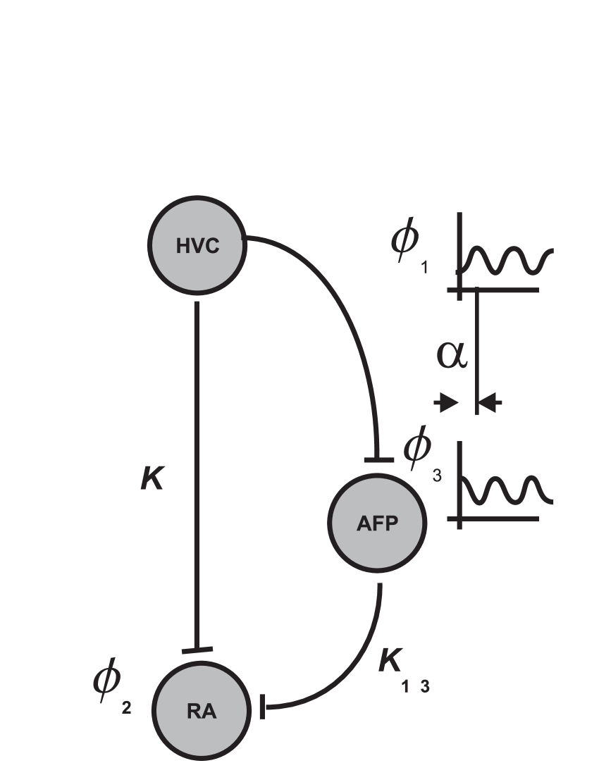
Figure 1: The activity of the nucleus HVC is represented by the phase variable $\phi_{1}$, and drives the neurons in nucleus RA through 2 different pathways: a direct way synapses onto the cells described by the phase variable $\phi_{2}$, and an indirect projection, controlling the activity of $\phi_{3}$ of another set of cells. The phase $\phi_{3}$ is delayed with respect to $\phi_{1}$ in $\alpha$. The strength $k$ of the connection between $\phi_{2}$ and $\phi_{1}$ depends on the phase difference $\phi_{2}-\phi_{1}$.

In contrast with the motor pathway, this pathway contributes only minimally to the production of song in adults [9]. However, it has been shown that the lesions to the nuclei in this pathway during learning profoundly alters the bird’s capability of developing normal song [10, 7]. The output of this pathway is the lateral magnocellular nucleus of the anterior neostriatum (LMAN). Individual RA neurons receive inputs from both LMAN and HVC nucleus, which is consistent with the picture that experience related LMAN activity facilitates certain HVC-RA synapses, helping to build the neural architecture necessary to produce the adult song. According to this picture, a sequence of bursts generated at a RA-projecting HVC will induce some activity in RA, and also eventually induce the activity of LMAN that will lead to either the potentiation or depression of the connection. This signal, however, requires a processing time through the AFP, which has been estimated in approximately $40$ $ms$ in Zebra finches [11].

If we are interested in the generation of the instructions controlling a motor output, it is sensible to model the process in terms of global oscillators. In this way, the periodic activity of the HVC nucleus when a syllable is being repeated is represented in terms of the oscillation of a simple oscillator. The nucleus RA, being driven by HVC, is represented by a second oscillator driven by the first one. In this framework, the dynamics of learning is the dynamics of the coupling coefficients between the oscillators.

With this biological inspiration, we make a computational study of the dynamical mechanisms by which a driven neural oscillator (representing the activity of a subpopulation of RA neurons) can learn to lock to its driver (representing the neurons in the nucleus HVC). The forcing that HVC performs upon RA through the indirect pathway AFP has been represented by a delayed reinforcement. The learned phase difference between driver and driven oscillators has been studied as a function of the reinforcement delay. In certain parameter regimes, small changes in the delay have been found to lead to important changes in the learned phase difference, and we explain this effect in terms of the dynamics of the system.

The work is organized as follows. In section 2 we discuss the mathematical model used to emulate the activities in our neural circuits. The solutions of this model are discussed in section 3. The consequences of the dynamical skeleton in terms of learning dynamics are discussed in section 4. Section 5 contains applications of these mechanisms to rate models of neural populations. Section 6 presents our conclusions.

2 Model

Rhythmic activity play an important role in many neural systems [13]. Cyclic neuronal activity is typically modeled in terms of periodic oscillators. Moreover, for those cases where the amplitude of the oscillations does not vary, it is possible to further reduce the dynamics of the oscillator to a phase variable. Winfree, Kuramoto and others have shown important features of coupled systems following this approach [12].

In a recent work, a generalized Kuramoto model of coupled oscillators with a slow coupling dynamics was investigated [13]. Inspired by a Hebbian like learning paradigm, the authors wrote a dynamical system for the evolution of the coupling which would strengthen synchronized states. The system of oscillators presented an interesting dynamics: the original difference between the natural frequencies of the oscillators served as a driving force in the dynamics of the phase differences between the oscillators. When the coupling parameters fell within a given range, the oscillators were eventually able to lock. In addition, a plasticity ingredient was incorporated, acting at a slower time scale. Namely, the dynamics of the coupling strength between the oscillators was driven by the phase difference between them. Once again, for some parameter values, the oscillators would end up locked.

In this work we are interested in the process of locking an oscillator to its driver, exploring the dynamical consequences of reinforcing the driving through a second pathway. In order to model this effect, three phase variables $\phi_{1}$, $\phi_{2}$ and $\phi_{3}$ are introduced. In terms of the inspiring problem, $\phi_{1}$ represents the oscillation of a first nucleus generating a periodic instruction (as HVC, with its periodic dynamics). The phase $\phi_{2}$ stands for the activity of some region of the nucleus RA, which contains premotor neurons controlling some aspect of the song production. This phase is driven by $\phi_{1}$. Finally, $\phi_{3}$ parametrizes the activity of the indirect pathway, and its dynamics is assumed to be the same as that of $\phi_{1}$, delayed some time $\tau$. Modelling the activity of HVC as a simple a harmonic function of frequency $\omega_{1}$, this delay translates into a phase $\alpha=\omega_{1}\tau$.

According to these hypothesis, the model describing the dynamics of these variables reads:

$$\frac{d\phi_{1}}{dt} = \omega_{1}$$ (1)

$$\frac{d\phi_{2}}{dt} = \omega_{2}-k\sin(\phi_{2}-\phi_{1})-k_{13}\sin(\phi_{2}-\phi_{3})$$ (2)

$$\frac{dk}{dt} = \gamma\cos(\phi_{2}-\phi_{1})-k$$ (3)

with $\phi_{3}=\phi_{1}-\alpha$.

In Fig. 1 we show a sketch of the three nuclei and their connections indicating the associated dynamical variables. Replacing $\phi_{3}=\phi_{1}-\alpha$ in Eq. 2, and scaling the equations, the following dynamical system for the phase difference $\phi_{2}-\phi_{1}=\phi$ and $k$ is obtained,

$$\frac{d\phi}{dt} = 1-k\sin\phi-k_{13}\sin(\phi+\alpha)$$ (4)

$$\frac{dk}{dt} = \epsilon(\gamma\cos\phi-k).$$ (5)

We are interested in understanding the dynamics of this set of equations, stressing on the stationary solutions that the system can “learn”. We are particularly interested in finding out whether there are delays that can provide any special advantage in the process of learning to control a periodic motor pattern.

3 Solutions

For a qualitative understanding of the solutions presented by this system of equations, we can compute the nullclines: curves for which each variable is stationary. They are:

$$k = [1-k_{13}\sin(\phi+\alpha)]/\sin\phi.$$ (6)

$$k = \gamma\cos(\phi)$$ (7)

In Fig. 2 we display the nullclines for different values

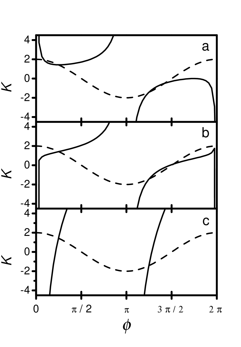
Figure 2: Nullclines $\dot{\phi}=0$ (full line) and $\dot{k}=0$ (dashed line), $\gamma=2$, $\alpha=3\pi/4$ and different values of $k_{13}$: (a) $k_{13}=1.5$, (b) $k_{13}=1$, and (c) $k_{13}=10$.

of the parameters. The intersections of the nullclines give the fixed points of the system $(k_{0},\phi_{0})$.

In the parameter range $k_{13}\in[0,1.42]$, the nullcline of Eq. (6) presents two branches: the first one with a minimum, the second one with a maximum. Depending on the parameter values, one of the branches or both might intersect the nullcline of Eq.(7). These intersections, when they occur, lead to the appearance of a saddle and a node in a saddle node bifurcation. For $\gamma$ sufficiently large, two attracting fixed points (separated by two saddles) can coexist. On the other hand, for $\gamma$ sufficiently small, there are no intersections between the nullclines and therefore, no stationary phase difference between the driver and the driven oscillator can be established.

The topological organization of the nullclines present qualitative changes as the system parameters are varied. These changes leave their imprint in the dependence of the stable fixed point angular positions with the parameters. In Fig. 3 we show the

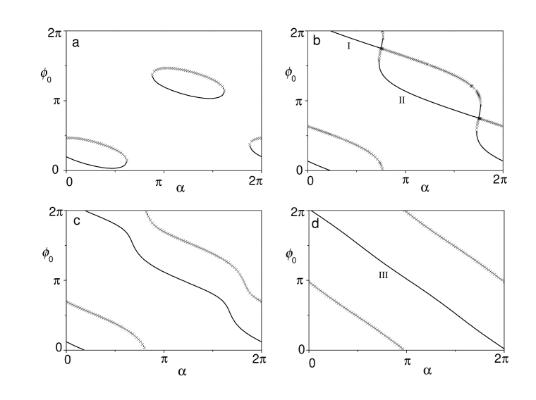
Figure 3: Stationary solutions for $\phi$ as a function of $\alpha$ for $\gamma=1$. Results for (a) $k_{13}=0.9$, (b) $k_{13}=1.5$, (c) $k_{13}=1.8$ and (d) $k_{13}=15$. In all the cases the solid lines correspond to stable solutions and the crosses indicate the branches of unstable solutions.

positions of the fixed points as a function of the reinforcement delay $\alpha$, varied between $(0,2\pi)$. The different insets correspond to a different value of the reinforcement parameter $k_{13}$. In the figure, the solid lines indicate the linearly stable solutions and the lines with crosses the unstable ones (which in all cases are saddle points). For small values of the coupling, there are delays for which no fixed points exist (Fig. 3a). At specific delays, stable and unstable fixed points are born in saddle node bifurcations. In terms of nullclines, this corresponds to situations in which the second nullcline of Eq.(6) presents a minimum which touches the nullcline of Eq. (7) (see Fig 2.a). As the reinforcement strength is increased, the region of reinforcement delays for which no stationary solutions exist decreases in size. As the reinforcement parameter $k_{13}$ is further increased, the regions with no solutions disappear and the bifurcation curves meet at a transcritic point (Fig. 3b) around which, a narrow zone of multistability appears. Finally, as the reinforcement strength is further increased, the angular position of the fixed points varies monotonically (Figs. 3c, 3d).

The existence of these bifurcation curves has profound consequences in terms of learning. Notice that close to certain values of the delay $\alpha$, a minimal change in $\alpha$ gives rise to important differences in the equilibrium phases learned by the system. In the following section, we will discuss potential consequences of this bifurcating structure in a learning process.

4 Interpretation

The animal model inspiring our dynamical model is the motor pathway in oscine birds. Part of this pathway is the nucleus RA containing excitatory neurons, some of which enervate respiratory nuclei, and others enervate the nucleus nXIIts, that projects to the muscles in the syrinx [14]. These two populations are segregated into different regions of the RA structure.

Recently, the study of the avian vocal organ allowed us to associate acoustical features of the song with properties of the muscle instructions necessary to generate the song. The production of repetitive syllables requires a cyclic expiratory gesture, and a cyclic gesture of the syringeal muscles [15]. Sound is produced by labia located at the junction between bronchii and tract, obstructing periodically the airflow . The model mentioned above describes the departure of the midpoint of a labium from the prephonatory position, $x$ [4, 8]:

$$\frac{dx}{dt} = y$$ (8)

$$\frac{dy}{dt} = -\epsilon(t)x-Cx^{2}y+B(t)y$$ (9)

where $\epsilon(t)$ is a function of the activity of ventral muscles, whereas $B(t)$ is a function of the bronchial pressure. This model has been tested, by using experimentally recorded $\epsilon(t)$ and $B(t)$. The resulting $x(t)$ was remarkably similar to the one produced while the physiological data had been recorded [8].

The phase difference between the $\epsilon(t)$ and $B(t)$, responsible for important acoustic features of song (such as the dynamics of the syllabic fundamental frequency) originates in RA. Recent work has unveiled that direct connections between respiratory nuclei and nXIIts can affect the final value of the phase difference. Yet, it is at RA that the neurons driven by HVC also receive input from the indirect pathway AFP, and therefore it is at this level that the phase difference between gestures can be altered.

In order to apply the results of the previous section to a learning strategy for birdsong, let us assume that two oscillators represent the cyclic activity of RA during the production of song. One of the oscillators mimics the activity of the neural population enervating the nXIIts nucleus, while the other oscillator represents the population of neurons which control the respiratory pattern. Both oscillators are assumed to be driven by the nucleus HVC, presenting a global activity with a syllabic rhythm. The reinforcement oscillator drives both RA oscillators with a signal equal to that of HVC, but delayed in a phase $\alpha$. Figure 4a illustrates the proposed architecture.

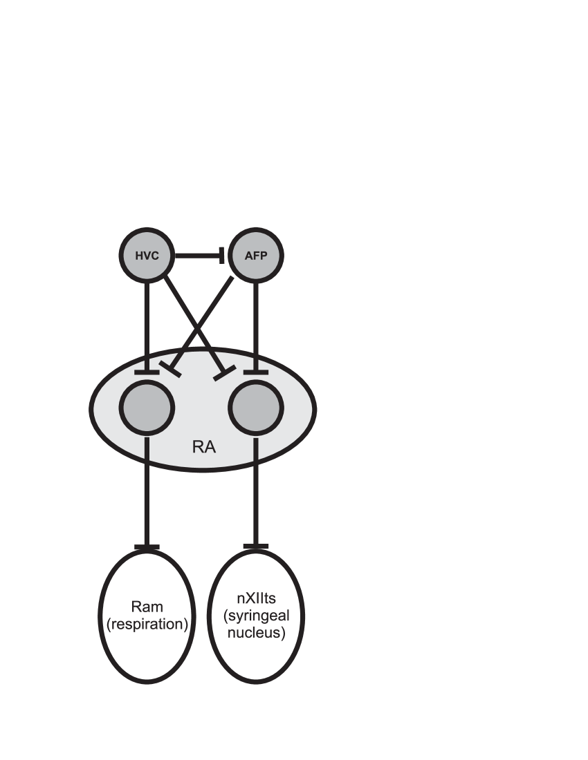
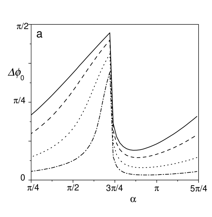
Figure 4: (a) Two oscillators representing neuron populations (nXIIts and RAm) driven by a master oscillator (HVC) will learn to follow the master at different delays. The two populations control different aspects of the song production apparatus: the syringeal nucleus and the respiratory muscles, respectively. (b) Phase difference $\Delta\phi_{0}$ as a function of $\alpha$. The solid line corresponds to the difference between the stationary solutions with $k_{13}=15$ and $k_{13}=1.5$; the dashed line to $k_{13}=5$ and $k_{13}=1.5$; the dotted line to $k_{13}=2.5$ and $k_{13}=1.5$; and the dashed-dotted line to $k_{13}=1.8$ and $k_{13}=1.5$. All calculations are performed with $\gamma=1$.

According to Fig. 3, if the two oscillators representing RA are strongly reinforced by the AFP circuit (i.e., if $k_{13}$ is large as in Fig. 3d), for every value of the forcing there will be a locked state. The phase difference between their own oscillation and the one of the driver will be the same for both oscillators, whatever the value of the delay $\alpha$. However, a different situation is found if each one of the oscillators is reinforced through a different coupling strength $k_{13}$. Imagine that for one of them, $k_{13}$ is similar to the one used to generate Fig. 3b, while the other one is forced though a coupling strength as the one used to generate Fig. 3d. In this case, depending on the value of the delay, qualitatively different phase differences can be achieved between each RA oscillators and the driver (and therefore, between the two RA oscillators themselves).

In Fig. 4b, the value of the phase difference $\Delta\phi_{0}$ is displayed as function of $\alpha$ for different pairs of oscillators. We have fixed $\gamma=1$. In all cases, one of the oscillators, which is taken as a reference, is assumed to be coupled to the AFP circuit through the parameter $k_{13}=1.5$, corresponding to the situation of Fig. 3b. For the other oscillator, we consider different values of $k_{13}>1.5$. All these couplings give rise to stationary solutions $\phi$ that decrease monotonously as a function of $\alpha$ (see Figs. 3c and 3d). The curves in Fig. 4b are the difference between the stationary solution of both oscillators, for several values of the second coupling constant. In order to indicate in detail how this difference is computed we take the example of the solid line in Fig. 4b, for which the second oscillator is coupled to the AFP circuit with a strength $k_{13}=15$. This curve corresponds to the difference of the solutions indicated with I and II in Fig. 3b (i.e. the stationary solution for the reference oscillator) and the curve III on Fig. 3d (the stable solution for the second oscillator). We notice, however, that there is a small range of $\alpha$ for which the branches of solutions I and II coexist. For such values of $\alpha$ we have taken branch II as the solution for the reference oscillator. This choice leads to the lowest possible value of phase difference between the two oscillators, since branch III is closer to branch II than to branch I. (Hence, the phase difference could be even higher than the one shown in Fig. 4b). It should be stressed that there are delays (close to the value $\alpha=3\pi/4$ for the parameters used here) for which small displacements can lead to a huge change in the stationary phase difference between the oscillators. Notice that Fig. 4b is $\pi$-periodic, so there is a similar effect around $\alpha=7\pi/4$.

The results in Fig. 4b, are robust with respect to changes in the parameter $\gamma$. We have checked that for all $\gamma\in(0.5,10)$, the transcritical bifurcation occurs at $\alpha\approx 3\pi/4$ and $\alpha\approx 7\pi/4$. Moreover, whenever $\alpha$ is in the neighborhood of any of these critical values, the phase difference between oscillators with different $k_{13}$ is highly sensitive to the value of $\alpha$. Yet, the values of $k_{13}$ relevant for observing the mentioned phenomena do depend on $\gamma$. For instance, the value of $k_{13}$ at which the transcritical bifurcation is observed increases with $\gamma$. It goes from $k_{13}\simeq 1.2$ for $\gamma=0.5$ to $k_{13}\simeq 6$ for $\gamma=10$.

Figure 5 illustrates how different the learned syllables can be

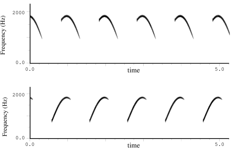
Figure 5: The sonograms of two songs which consist of a repetition of the same syllable, for which the phase difference learned is (a) $\Delta\phi_{0}=0$ and (b) $\Delta\phi_{0}=\pi/2$. The parameters of Eqs. 8 and 9 are $\epsilon(t)=7\,10^{7}+6\,10^{7}cos(2\pi t/44100)$ a.u, $B(t)=5\,10^{2}+10^{3}cos(2\pi t/44100+\Delta\phi_{0})$ a.u, $C=2\,10^{9}$ a.u.

for small changes in the reinforcement delay, if they occur around $\alpha=3\pi/4$. The figure displays a sonogram showing the time evolution of the fundamental frequency of the sound produced by the model of the syrinx, when driven by the “learned” phase differences.

5 Application to rate models

The Kuramoto model describing the time evolution of phase differences between oscillators constitutes a popular model, particularly suited for analytic work. Yet, we explored whether these effects are also present in other models. We tested the basic findings of the previous sections in rate models for the activities of neural populations.

Rate models are introduced to account for the dynamics of the average activity of neural nuclei. For a problem involving a macroscopic motor control program it is a suitable level of description. In particular, a widely used model for the average activity of two subpopulations (exitatory and inhibitory) is the Wilson Cowan system of equations [16].

We let $x$ and $y$ stand for the activities of the excitatory and inhibitory subpopulations respectively. In [14] it was shown that in the portions of RA with neurons projecting to XIIts and to respiratory nuclei, the (excitatory) projecting neurons coexist with inhibitory neurons. We drove the equations ruling their dynamics with two signals. One represents HVC activity and the other one, the activity in nucleus LMAN, assumed to be a delayed copy of the first signal. A typical hebbian rule was used to describe the dynamics of the coupling between HVC and RA. The system reads

$$\frac{dx}{dt} = -x+S[\rho_{x}+ax+by+k\cos(\omega t)+k_{13}\cos(\omega t-\alpha)]$$

$$\frac{dy}{dt} = -y+S(\rho_{y}+cx+dy)$$ (10)

$$\frac{dk}{dt} = \lambda x\cos(\omega t)-k$$

with a saturation function $S(x)=1/(1+e^{-x})$.

We integrated these equations for the whole range of delays $\alpha\in[0,2\pi)$. In Fig. 6 we show a window representing a

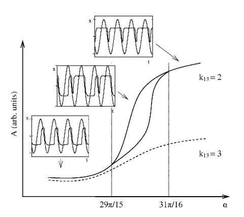
Figure 6: Bifurcation diagram for the Wilson-Cowan system (Eq. 10) forced with frequency $\omega=0.3$. The horizontal axis represents the delay $\alpha$ and the vertical axis represents the maximum amplitude $A$ of the oscillations in phase space. A broad phase difference between two slave oscillators with weights $k_{13}=2$ and $k_{13}=3$ can be achieved within a narrow range of delays $29\pi/15<\alpha<31\pi/16$. On the insets, solutions $x(t)$ along with forcing function $cos(\omega t)$ for the three different regimes found. The equations were integrated with the following parameters: $\rho_{x}=-5.75$, $\rho_{y}=-1$, $a=10$, $b=-1.5$, $c=2$, $d=2$ and $\lambda=68$.

bifurcation around $\alpha=29\pi/15$, where two qualitatively different period-one solutions can be found. The transition occurs through a bubble in parameter space where a period-two exists. It is interesting that the different period-one solutions (illustrated in the insets), are locked to the periodic forcing frequency at different phases. As $k_{13}$ is increased, only a single period-one solution is present. Therefore, two subpopulations reinforced through a delay $\alpha$ around this bifurcating value with these weights will lock at a phase difference within a wide range of values as the delay is slightly increased.

6 Conclusions

In a recent work [13], the process of learning a phase difference between two phase oscillators coupled with a slow varying coupling constant was described. Here, the impact of subjecting the driven system to two delayed copies of a signal is studied. This design is inspired in an animal model, oscine birds, which learn their song by modifying the architecture of connections within the motor pathway. Our model is a caricature of the complex processes that have been described for the animal model, which involved the convergence to a motor nucleus of two signals, separated by a delay. Our study indicates that for some values of the amplitude of the reinforcement, the learned phase difference between driver and slave depends strongly on the delay of the reinforcement. This allows to conceive simple strategies of learning motor gestures that require a tuning between different neural populations. We precisely illustrate the power of this strategy with an example of the inspiring biological problem. We show that playing with small variations in the delay of the reinforcement, completely different syllables in a bird song can be generated.

In the problem of bird song learning, the timing of the indirect pathway (the anterior forebrain pathway) can be changed [17] by dopaminergic input. Not much is known about the precise nature of the coding used by a bird to translate an error into the indirect signal. Measures of activity in the nucleus LMAN (the last one of the AFP pathway, which projects onto RA) in a juvenile bird learning his song are still not possible. The simple model presented in this work allows us to explore theoretically the dynamical mechanisms that enter into a learning scheme compatible with the basic ingredients present in the animal model. Moreover, it provides a new control mechanism applicable to artificially designed neural systems.

References

- [1] Brainard M.S., Doupe A.J., Nature Reviews 1 31 (2000)
- [2] Brainard M.S., Doupe A.J., Nature 417 351-358 (2002)
- [3] Abarbanel H. D. I. A, Gibb L., Mindlin G. B., Rabinovich M., and Talathi S. J. Neurophysiol. 92 96-110 (2004)
- [4] Gardner T., Cecchi G., Magnasco M., Laje R. and G. B. Mindlin, Phys. Rev. Letts., 87 art. 208101 (2001)
- [5] Nottebohm F., Stokes T. M. and Leonard C. M. J. Comp. Neurol. 165 457-486 (1976).
- [6] Hahnloser R. H. R., Kozhevnikov A. A. and Fee M. S Nature 419 65-70 (2002).
- [7] Scharff C. and Nottebohm F., J. Neurosci. 11 2896-2913 (1991).
- [8] Mindlin G. B., Gardner T. J., Goller F., Suthers R. Phys. Rev. E,68 041908 (2003).
- [9] Kimpo R.R., Theunissen F. E., Doupe A. J. J. Neurosci. 23 5750 (2003)
- [10] Bottjer S., Miesner E. A., Arnold A. P., Science 224 901-903 (1984).
- [11] Brainard M. and Doupe A. J. Nature 417, 351 - 358 (2002)
- [12] Pikovsky A., Rosemblum M. G. and Kurths J. Synchronization: a universal concept in nonlinear sciences. Cambridge Nonlinear Science 12, Cambridge University Press, Cambridge (2000).
- [13] Seliger P, Young S. C. and Tsimring L. Phys. Rev. E 65 041906 (2002)
- [14] Spiro J. E., Dalva M. B. and Mooney R. J. Neurophysiol. 81 3007-3020 (1999).
- [15] Gardner T., Cecchi G., Magnasco M., Laje R. and Mindlin G. B. Phys. Rev. Letts. 87 art 2008101 1-4 (2001).
- [16] Hoppensteadt F. and Izhikevich E., Weakly Connected Neural Networks, Springer, 1997.
- [17] Abarbanel H. D. I. A., Talathi S., Mindlin G. B., Rabinovich M. and Gibb L. Physical Review E 70 168409 (2004)