Study of Arbitrary Nonlinearities in Convective Population Dynamics with Small Diffusion

Abstract

Convective counterparts of variants of the nonlinear Fisher equation which describes reaction diffusion systems in population dynamics are studied with the help of an analytic prescription and shown to lead to interesting consequences for the evolution of population densities. The initial value problem is solved explicitly for some cases and for others it is shown how to find traveling wave solutions analytically. The effect of adding diffusion to the convective equations is first studied through exact analysis through a piecewise linear representation of the nonlinearity. Using an appropriate small parameter suggested by that analysis, a perturbative treatment is developed to treat the case in which the convective evolution is augmented by a small amount of diffusion.

I Introduction

The Fisher equation, proposed originally to describe the spread of an advantageous gene in a population fisher1937 , has found a great deal of use in mathematical ecology, directly murray ; skellam ; kk ; bkk as well as indirectly, i.e., in modified forms. Examples of modifications are the incorporation of internal states such as those signifying the presence or absence of infection ak ; akyp ; kpasi , the introduction of temporal nonlocality in the diffusive terms manne ; abk , of spatial nonlocality in the competition interaction terms fkk ; fk , and the addition of convective terms signifying ‘wind effects’ nelson ; ana ; gk ; lgthesis ; k . Most of the modifications lead to equations which, as in the case of the original Fisher equation, are not soluble analytically and require approximate or numerical methods for their analysis. There is, however, one modification gk , that leads to an analytic solution via a trivial transformation, and to the possibility of the extraction of interesting information of potential use to topics such as bacterial population dynamics. That modification consists of the replacement of the diffusive term in the Fisher equation

$$\frac{\partial\,u}{\partial t}=au\left(1-\frac{u}{K}\right)+D\frac{\partial^{2}\,u}{\partial x^{2}}$$ (1)

by a convective term. As is well-known, in the original Fisher equation, $u$ represents a concentration or density, $a$ the growth rate, $K$ the so called ‘carrying capacity’, and $D$ the diffusion constant. In spite of the fact that purely convective (non-diffusive) nonlinear partial differential equations are much less sophisticated than their diffusive counterparts, there are at least two reasons why their study is important. There are clear physical situations nelson ; ana ; gk in which wind effects which add the convective term to a diffusive equation are present. These arise, for instance, when one changes one’s reference frame to that of a moving mask in bacterial population dynamics experiments nelson . Because the convective term comes from the macroscopic motion of the mask under experimental control whereas the diffusive term comes from the microscopic motion of the bacteria, it is possible to arrange the system experimentally so that the diffusion effects are relatively unimportant. This may be achieved for instance, by using viscous environments, or by genetically engineering the (bacterial) population. In such a case one arrives at the analysis of a largely convective (negligibly diffusive) nonlinear evolution which may be investigated in zeroth order as a purely convective equation gk ; k . This fact, that experimental realization of the convective nonlinear equation is indeed possible, provides one motivation for these studies. The other, as explained in Ref. gk , is that it is possible to develop perturbation schemes starting from the soluble convective equation to incorporate diffusive effects. In Sections II and III, we develop the theory for arbitrary nonlinearities in the absence of the diffusion constant, and in Section IV, we focus on the effect of adding the diffusive term.

Recently, a simple prescription for generalizing the analysis of Ref. gk was given by one of the present authors k to arbitrary nonlinearities in the convective equation. The equation considered there is

$$\frac{\partial\,u}{\partial t}+v\frac{\partial\,u}{\partial x}=auf(u),$$ (2)

where $v$ is the medium or ‘wind’ speed, $a$ is a growth rate and $f(u)$ is a dimensionless arbitrary nonlinearity. The prescription provided in that analysis gives the full time and space evolution of $u(x,t)$ in terms of its initial distribution $u(x,0)=u_{0}(x)$, through the relation

$$u(x,t)=G^{-1}\big{[}G[u_{0}(x-vt)]-at\big{]}$$ (3)

where the function $G(u)$ is obtained from the nonlinearity $f(u)$ by the integration k

$$G(u)=-\int\frac{1}{uf(u)}du.$$ (4)

We have used a slightly changed notation here relative to ref. k . Our functions $G(u)$ and $f(u)$ are both dimensionless in contrast to the dimensioned counterparts $g(u)$ and $F(u)$ in ref. k .

In this paper we present several applications of the prescription (3) and report a number of additional results from the nonlinear convective equation (2). In Section II, we examine features of the solutions obtained exactly from the prescription for several cases of the nonlinearity including an interesting ‘pyramid effect’ that occurs for nonlinearity functions $f(u)$ with multiple zeros. In Section III, we develop a general analysis for finding traveling wave solutions, and to study characteristics of the tails and shoulders of such solutions. Applications of this analysis for the nonlinearities studied in Section II are also made in Section III. In Section IV, we analyze in detail the perturbative problem obtained by adding a small amount of diffusion to the nonlinear convective equation. Conclusions are presented in Section V.

II Applications of the Prescription for the Solution of the Initial Value Problem

Applications of the prescription (3) for the solution of the arbitrary initial value problem were indicated in ref. k for three cases: the ordinary logistic nonlinearity for which $f(u)$ has a single zero at $u=K$, the Nagumo nonlinearity for which $f(u)$ has two zeros, and the trigonometric nonlinearity for which $f(u)$ has multiple zeros. We will display new results for the latter two, and analyze other generalizations of the logistic nonlinearity. In some of these cases (subsections A,D and E below) $u(x,t)$ is presented in an implicit form, whereas in the others (subsections B and C) the form is given explicitly.

II.1 Allee effect from Nagumo nonlinearity

In (2) let $f(u)$ be given by

$$f(u)=\left(1-\frac{u}{K}\right)\left(\frac{u}{K}-\frac{A}{K}\right)$$ (5)

where $A<K$. Such an $f(u)$ represents the so called ‘Allee effect’. This effect allee is associated with the existence of an additional zero (fixed point) in the nonlinearity relative to the logistic case. Unlike in the logistic case, the zero-$u$ solution is stable here. If $u$ is small initially, it is attracted to the vanishing value; if large, it is attracted to the non-zero value $u=K$. The demarcation point is the additional zero introduced in this case, viz. $u=A$. The physical origin of the Allee effect in population dynamics is the possible increase of survival fitness as a function of population size for low values of the latter. Existence of other members of the species may induce individuals to live longer whereas low densities may, through loneliness, lead to extinction. There is ample evidence for such an effeect in nature courchamp ; SS ; fowlerbaker .To construct $G(u)$ from (4) is straightforward,

$$G(u)=\frac{1}{A(K-A)}\ln\left(\frac{(K-u)^{A}u^{K-A}}{|u-A|^{K}}\right),$$ (6)

but to invert $G(u)$ is not. In Fig. (1) the nonlinearity is displayed along with the time evolution for a certain initial condition. The Allee effect causes a decay to zero of parts of the solution, while other parts evolve to the saturation value K. Thus, an initial condition with $u$ values belonging to both regions, will show a growth for those points in space such that $u_{0}(x)>A$, while those points such that $u_{0}(x)<A$ will decay to zero. The initial condition in this case evolves into a step profile of width given by the separation in space of the two points where $u_{0}(x)=A$.

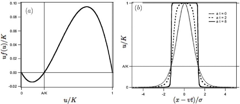
Figure 1: The Nagumo nonlinearity of Eq. (5) and its effects on evolution. The nonlinearity is plotted in (a). Shown in (b) is an example of the evolution from an initial condition $\textrm{sech}(x/\sigma)$ (shown by the dotted line) whose profile belongs both to the region where $0<u(x)<A$ and where $A<u(x)<K$. The portion in the first (lower) region decays while that in the second (upper) region grows to the saturation value $u(x)=K$. Here, $\sigma$ is an arbitrary length.

II.2 Trigonometric nonlinearity and the Pyramid Effect

What would happen if the nonlinearity function $uf(u)$ had multiple zeros rather than three as in the Nagumo case? The physical origin of such behavior may lie in nonmonotonic response of survival fitness to population size. Complex biological and sociological interactions among members of the species could exist on the basis of the coupling of mating instincts with mere size effects. Such interactions could, in principle, make the survival fitness optimum at several, rather than a single, values of the population size. In order to address such situations, extensions of the normal Allee considerations are necessary. For this purpose, the discussion in A above may be generalized as follows. For a given nonlinearity with an arbitrary number of zeros, $uf(u)$ can be sectioned among each subsequent unstable zero. The dynamics of each point of the initial profile will evolves according to which of these sections it belongs initially. In the Nagumo case there are only two such regions: the first region is between $u=0$ and $u=A$, while the second region is for $u>A$. All the points of the initial condition such that $u_{0}(x)<A$ decay to zero, while all those points belonging to the second region grow to the saturation value $u=K$. But when there is more than one unstable zeros, as in the case of a trigonometric nonlinearity, the propagating solution may evolve into a pyramidal profile. To show this we choose a sinusoidal nonlinearity given by

$$f(u)=\frac{K}{\pi}\frac{\sin\left(\frac{\pi u}{K}\right)}{u}$$ (7)

where we took the opportunity to change the stability of $u=0$ compared with the Nagumo case presented in A. From (4), $G(u)$ is given by

$$G(u)=-\ln\left[\tan\left(\frac{\pi u}{2K}\right)\right]$$ (8)

and the exact solution at all time is

$$u(x,t) = \sum_{m=1}^{+\infty}K\left(1-\frac{2}{\pi}\arctan\left[e^{-at}\cot\left(\frac{\pi}{2K}\left\{\Theta\left[\frac{2mK}{\pi}-u_{0}\left(x-vt\right)\right]\right.\right.\right.\right.$$ (9)

$$\left.\left.-\Theta\left[\frac{\left(2m-2\right)K}{\pi}-u_{0}\left(x-vt\right)\right]u_{0}\left(x-vt\right)\right)\right]+\left(m-1\right)\times$$

$$\left.\left\{\Theta\left[\frac{2mK}{\pi}-u_{0}\left(x-vt\right)\right]-\Theta\left[\frac{\left(2m-2\right)K}{\pi}-u_{0}\left(x-vt\right)\right]\right\}\right).$$

Let us consider an initial condition such that $0<u_{0}(x)<2mK$ where $m$ is a positive integer. All those initial points of the profile that belong to the region delimited by $(2m-2)<u(x)<2mK$ can be described by the following dynamics. The solution grows from $u=(2m-2)K$ to the value $u=(2m-1)K$ and decays to it from $u=2mK$ following the evolution of an initial condition with compact support in that region. As extensively studied in the case of the logistic nonlinearity gk , any initial condition with a bounded domain evolves into a step profile of width given by its initial value. In the sinusoidal nonlinearity, from each region a step profile with width given by $\Theta\left[2mK/\pi-u_{0}(x)\right]-\Theta\left[(2m-2)K/\pi-u_{0}(x)\right]$ eventually emerges. Figure (2) shows an example for an initial condition that overlays three such regions. It is clear from the figure that in the bottom region the profile behaves as if the other regions did not exist.

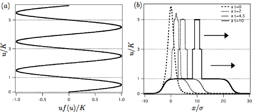
Figure 2: The ‘pyramid effect’ for a nonlinearity with multiple zeros. The sinusoidal nonlinearity of Eq. (7) is plotted in (a). The horizontal lines at $u/K=1,3,5$ depict levels of separation of the regions between stable zones. The corresponding evolution is plotted in (b) for the initial profile $u_{0}(x)=5.9\,K\,\textrm{sech}(x/\sigma)$, where $\sigma$ is an arbitrary length. The initial profile is shown as a dotted line. The profile moved rightwards as shown.

II.3 Multi-individual struggle for environment resources: linear growth with power saturation

One can envisage physical situations in which one encounters a simple generalization of the logistic nonlinearity that retains the linear behavior near $u=0$ but accentuates the nonlinearity for larger values of $u$. This would arise, e.g., if the elemental struggle of the individuals for resources involves not two but multiple individuals. The struggle would then not be binary in nature. To address this possibility, we consider

$$f(u)=\left[1-(u/K)^{n}\right].$$ (10)

The saturation effect already seen in the logistic case, becomes more abrupt as $n$ increases. Pictorial representations for several cases of $n$ are provided in Fig. (3). Application of the prescription (4) produces the explicit form for $G(u)$

$$G(u)=\frac{1}{n}\ln\left[\frac{1-(u/K)^{n}}{(u/K)^{n}}\right].$$ (11)

Its inverse can be written analytically. An arbitrary initial condition $u_{0}(x)=u(x,0)$ therefore via prescription (3) evolves according to

$$u(x,t)=\frac{u_{0}(x-vt)}{\left[\left(\frac{u_{0}(x-vt)}{K}\right)^{n}(1-e^{-ant})+e^{-ant}\right]^{1/n}}.$$ (12)

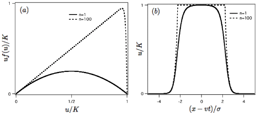
Figure 3: The nonlinearity with power saturation and its effect on the time evolution. The nonlinearity with $f(u)$ given by (10) is shown in (a) for two different powers $n$. Near $u=0$ both functions are similar but for higher values they differ dramatically since the case $n=100$ has an abrupt drop close to $u=K$. Their corresponding time evolution is plotted in (b) at a time $at=5$ starting from the same initial condition $K\textrm{sech}(x/\sigma)$ where $\sigma$ is an arbitrary length.

II.4 Nonlinear growth with power saturation as in bisexual reproduction

Interesting consequences arise if the nonlinearity cannot be approximated by a linear term near $u=0$, such as when the growth of the species is nonlinear. A physically relevant example is the representation of bisexual reproduction that would require a growth term bilinear rather than linear (see for example Ref. rosas2002 ). The generalization of the nonlinearity (10) to a nonlinear growth term can be expressed as

$$f(u)=(u/K)^{m}\left[1-(u/K)^{n}\right]$$ (13)

where $m+1$ is the first power in $u$ in a Taylor expansion near zero. Prescription (3) gives

$$G(u)=\frac{{}_{2}F_{1}\left[1,-\frac{m}{n},1-\frac{m}{n},\left(\frac{u}{K}\right)^{n}\right]}{Km\left(\frac{u}{K}\right)^{m}}.$$ (14)

where ${}_{2}F_{1}$ is the hypergeometric function. In general, Eq. (14) cannot be inverted and $G^{-1}$ has to be calculated implicitly. However, analytical considerations regarding the shape of tails and shoulders of traveling fronts can be easily obtained through the help of Eq. (14) as will be seen below in Sec III.

II.5 Nonlinearity with provisional saturation

The previous nonlinearities we have discussed above increase (decrease) monotonically from one zero to a maximum (minimum) and then monotonically decrease (increase) to the next zero. Our prescription (3) permits the analysis of more interesting situations that may arise if the mutual struggle for resources among individuals constituting the species leads to saturation of the population size that is not permanent but only provisional. Further increase in the population density in such a situation might lead to a returned increase in the nonlinearity, followed by an eventual decrease. Such a state of affairs is analogous to the case analyzed in subsection B above but with an important difference. In the present case, $uf(u)$ does not dip below zero. As a consequence, there are no multiple zeros at $u\neq 0$. In Fig.(4) we present, as an example of such a nonlinearity, a polynomial of the form,

$$uf(u)=9(u/K)-\frac{131\,(u/K)^{2}}{12}+\frac{9\,(u/K)^{3}}{2}-\frac{7\,(u/K)^{4}}{12}$$ (15)

and the corresponding time evolution. As time evolves, the curvature of the solution reflects the specific particulars of the “reaction” term. In the solution the regions with $u$ values close to the top of the reaction function have more inclination.

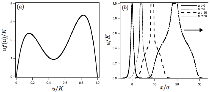
Figure 4: Example of a nonlinearity with provisional saturation. In (a) the reaction function $uf(u)/K$ of the polynomial 15 is presented, while in (b) the corresponding evolution for an initial condition is shown.

To study the effects of different dips, in Fig.(5) three similar $uf(u)$ are shown which differ in the ’depth’ of their valleys. Their construction is straightforward by means of the Lagrange interpolating polynomial, i.e. by taking a polynomial of fourth order and requiring it to have specific values at the five points desired. In the example of the figure, four of the five points that are required to be common are: $(0;0),(1;0),(1/4;1),(3/4;1)$ described in $(u/K;uf(u))$ plane. The other point will characterize the dip, and for the example shown in the figures are $(1/2;9/10),(1/2;1/2),(1/2;1/10)$. From the same initial condition, the evolution will differ as shown in (b): the more pronounced the dip in the nonlinearity, the flatter the solution close to the center of the dip.

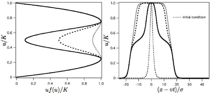
Figure 5: Dependence of the depth of the dip for nonlinearities with provisional saturation. In (a) three different nonlinearities are plotted. The axis are interchanged respect to the previous figure. This has been done to express clearly the correspondence between the nonlinearities in (a) and the evolution in (b).

III Traveling Front Solutions: Analytical expressions for spatial limits

The analysis in the previous section has focused on the initial value problem. Much interesting information in nonlinear problems may be extracted, however, directly from traveling waves (see, e.g., extensive reports in the soliton literature such as in soli ). The $G$-function appearing in our prescription (3) can be used conveniently, and directly, to find traveling wave solutions. As will be seen below, there are situations in which this technique is useful even when explicit analytic expressions cannot be found for the initial value problem. Imposing the traveling wave ansatz $u(x,t)=U(z=x-ct)$ in Eq.(2),

$$-\beta\frac{\partial\,U}{\partial z}=aUf(U),$$ (16)

where

$$\beta=c-v$$ (17)

is the difference between the traveling front velocity and the medium velocity. Integrating (16) in $z$, leads to the solution

$$G\left[U_{\beta}(z)\right]=a\frac{z}{\beta},$$ (18)

where $G$ is defined in Eq. (4). If the function $G^{-1}$ can be written analytically, the front solution can be obtained in explicit form:

$$U_{\beta}(z)=G^{-1}\left[a\frac{z}{\beta}\right].$$ (19)

Otherwise it is defined implicitly through Eq. (18).

Equation (19) shows that, for a given nonlinearity, the steepness of the front depends on the propagation velocity $c$ while its shape is determined by the function $G^{-1}$. In order to show how, for a given propagation velocity $c$, the shape of the front changes for various nonlinearities (according to the simple relation (19)), we provide Fig. (6).

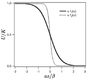
Figure 6: Example of several traveling waves of the same speed, $\beta=1$, but for different nonlinearity functions $f$. The solid line is the generalized logistic function, $uf_{1}(u)=u(1-u^{2})$, while the dotted line comes from the first half period of the sinusoidal function, $uf_{2}(u)=sin(\pi u)$.

We now show how one may find analytic expressions for the tail and the shoulder of the traveling wave through inspection of the limiting values of the nonlinearity $auf(u)$, respectively, as $u\to 0^{+}$ and $u\to K^{-}$, where $0$ and $K$ are both zeros of the nonlinearity. The basic idea is to apply to Eq. (18) a judiciously chosen function $h$, multiply by $U$ or $(K-U)$ as appropriate, and then calculate the relevant limit of the product. Thus, if we are interested in the spatial dependence of the tail of the solution, we seek to obtain

$$\lim_{U\to 0^{+}}U(z)h_{T}\left(G\left(U\right)\right)=\lim_{z/\beta\to+\infty}U(z)h_{T}(az/\beta)=C_{T}.$$ (20)

The function $h_{T}$ is chosen in such a way that the limit for $U\to 0^{+}$ of the left hand side of the equation equals a non zero constant depicted above by $C_{T}$. If the shoulder spatial dependence is sought, we apply another function $h_{S}$, and multiply by $(K-U)$ rather than by $U$ before taking the limit $U\to K^{-}$, the choice of $h_{S}$ being such that the limit is a constant $C_{S}$.

The spatial dependence of the traveling solution in the two extreme limits is found to be

$$\lim_{z/\beta\to+\infty}U(z)\simeq\frac{C_{T}}{h_{T}\left(az/\beta\right)}$$ (21)

for the tail and

$$\lim_{z/\beta\to-\infty}U(z)\simeq K-\frac{C_{S}}{h_{S}\left(az/\beta\right)}$$ (22)

for the shoulder.

The steepness of the front at the inflection point is another important feature of the traveling front that can be obtained from the shape of the nonlinearity even if the exact analytic form is not known. From Eq. (16) we can simply relate

$$\frac{dU(z)}{dz}=-aU(z)\frac{f\left[U(z)\right]}{\beta}.$$ (23)

which clearly shows the relation between the maximum of $f(u)$ and the front derivative at the inflection point. Comparing such values with those cases of $f(u)$ in which the traveling front shape are known analytically, allows to determine further qualitative characteristics of the front shapes. We apply these various general considerations to two specific cases below.

III.1 Linear growth with power saturation

From the general expression (3), it is straightforward to write the analytic form of the traveling fronts

$$U_{\beta}(z)=\frac{K}{\left(1+\left(2^{n}-1\right)e^{an\frac{z}{\beta}}\right)^{1/n}},$$ (24)

where we have chosen to center the traveling front in such a way that $U_{\beta}(z=0)$ is half the saturation value of $U$. Application of the limiting procedure described above shows that regardless of the value of the power saturation $n$ the front tail is given by

$$\lim_{z/\beta\to+\infty}U_{\beta}(z)\propto e^{-az/\beta}.$$ (25)

The value $n$ does not play a role since the tail shape is determined by the form of the nonlinearity close to $U=0$ where saturation effects are negligible. On the other hand, the value $n$ does play a role in determining the shoulder shape. The limiting procedure gives in fact

$$\lim_{z/\beta\to-\infty}U_{\beta}(z)\propto K-\frac{K}{n}e^{-az/\beta}.$$ (26)

which coincides with the one calculated directly from Eq. (24).

It is interesting to notice that in the limiting case corresponding to $n\to\infty$ the traveling front solution can be written as

$$U_{\beta}(z)=\left\{\begin{array}[]{ll}K&\textrm{if }z\leq 0\\ Ke^{-z/\beta}&\textrm{if }z>0\end{array}\right.$$ (27)

III.2 Nonlinear growth

For the case in which the growth near $u\sim 0$ is bilinear as in (13) for $m=2$, the prescription (3) is given in terms of hypergeometric functions (see Ref. hypergeometric ), whose inverses are not known. However our limit prescriptions (21) and (22) do provide analytical expressions for the spatial limits. For $U\approx 0$ the following behavior is obtained

$$G(u)\propto\frac{1}{Km(U/K)^{m}}.$$ (28)

The function $h_{T}$ of Eq.(20) which makes the left limit a constant is found to be

$$h_{T}(G)=G^{\frac{1}{m-1}}.$$ (29)

Therefore, in the tail,

$$\lim_{z/\beta\to+\infty}U(z)\simeq\frac{C}{(z/\beta)^{\frac{1}{m-1}}}.$$ (30)

Indeed, we can determine the shape of the tail (shoulder) for any function $f$ that has a Taylor expansion near $U=0$ ($U=K$).

IV Incorporation of diffusion along with convection

The analytic treatment we have given above of the reaction-convection problem represented by Eq. (2) has been made possible by the fact that the partial differential equation considered is of first order. Once the transformation is made to convert (2) exactly into its linear counterpart, the method of characteristics char , well-known in the context of linear equations, is what is behind the analysis we have presented. If diffusion is added to (2), individual points of the $u(x)$ curve at a given time no longer evolve independently as they do for systems characterized by (2) but influence one another in the evolution. Finding analytic solutions in the manner detailed here and in Refs. gk ; k is then impossible. There is no doubt from the practical viewpoint that the case $D=0$ is important to study. This is so because negligible diffusion does occur in several physical situations as in the case of bacterial dynamics when the environment or genetic engineering can be made to result in convection being far more important than diffusion. Nevertheless it is important to ask whether the introduction of diffusion can be considered a perturbation or whether it alters the problem drastically, even when it is relatively small in magnitude. If the latter were true, the analysis presented in the previous sections would be uninteresting for all realistic cases in which finite diffusion exists. We therefore analyze the effects of adding diffusion to the nonlinear convective problem:

$$\frac{\partial\,u}{\partial t}+v\frac{\partial\,u}{\partial x}=auf(u)+D\frac{\partial^{2}\,u}{\partial x^{2}}.$$ (31)

We do this in three parts, always focusing attention on traveling wave solutions for simplicity. In the first part (subsection A below), we obtain exact analytical expressions for traveling wave solutions of the reaction diffusion problem represented by equation (31) when $f$ is a piecewise linear function. Also, we compare the results between the absence of diffusion to those in its presence (arbitrary amount of diffusion). In the second part, when the amount of diffusion is small, we identify an appropriate small parameter and develop a perturbation scheme. In the third part, we apply the perturbation treatment to one of the interesting nonlinearities (sinusoidal) introduced at the beginning of this paper. Furthermore, we analyze its validity by comparing it to the exact solution of (31) when the nonlinearity is piecewise linear. The last two parts make up subsection B below.

IV.1 Diffusion effects treated through a piecewise linear representation of the nonlinearity

Although exact analytic solutions of the nonlinear equation we consider are impossible in the presence of diffusion, they are possible for traveling waves if we employ a piecewise linearization of the nonlinearity. The piecewise linear approximation has been used earlier in the analysis of the Fisher equation for the study of the effects of transport memory manne as well as pattern formation horacio . In both cases it was possible to extract useful information through this resource, whose advantage is that once the approximation of representing the given nonlinearity by the piecewise linear form is made, no further approximation is invoked. Let us begin with a piecewise representation of the logistic nonlinearity through

$$f(u)=\left\{\begin{array}[]{ll}1&u/K\leq\alpha\\ \left(\frac{\alpha}{1-\alpha}\right)\left(\frac{1-u/K}{u/K}\right)&u/K\geq\alpha,\end{array}\right.$$ (32)

in which the first piece of $uf(u)$ connects the unstable zero at $u=0$ to the maximum at $u=\alpha K$, while the second piece joins the maximum with the stable zero at $u=K$. The parameter $0\leq\alpha\leq 1$ in (32) represents the relative position of the maximum of the nonlinearity between the stable and unstable zeros of the system. If $\alpha=1/2$, the derivatives of the logistic nonlinearity and its piecewise representation become equal at $u=0$ and $u=K$. Since the tail of a front solution is determined by the limit (21), the choice $\alpha=1/2$ ensures that the spatial dependence of the tail (shoulder) front in the logistic nonlinearity coincides with the tail (shoulder) front when $f(u)$ is given by (32). In the analytic treatment below, for the sake of generality, we keep the parameter $\alpha$ unspecified.

Following the method of Ref. manne it is straightforward to determine the exact form of the traveling wave solution of Eq. (31) with $f$ given by (32). Such a solution, denoted as $U(z,\gamma)$, where $\gamma=v_{f}/\beta$ and $v_{f}=2\sqrt{Da}$ is given by

$$U(az/\beta\leq 0,\gamma) =K-K(1-\alpha)\,\exp\left(\frac{az}{\beta}/\lambda_{1}\right),$$ (33a)

$$U(az/\beta>0,\gamma) =B_{2}\,\exp\left(-\frac{az}{\beta}/\lambda_{2}\right)+B_{3}\,\exp\left(-\frac{az}{\beta}/\lambda_{3}\right),$$ (33b)

with

$$\lambda_{1} =(2/\gamma^{2})\left(\sqrt{1+\frac{\alpha}{1-\alpha}\gamma^{2}}-1\right), B_{2} =(1/2)K\left(\alpha-\xi\right),$$ (33c)

$$\lambda_{2} =(2/\gamma^{2})\left(1+\sqrt{1-\gamma^{2}}\right), B_{3} =(1/2)K\left(\alpha+\xi\right),$$ (33d)

$$\lambda_{3} =(2/\gamma^{2})\left(1-\sqrt{1-\gamma^{2}}\right), \xi =-(1-\alpha)\frac{\sqrt{1+\frac{\alpha}{1-\alpha}\gamma^{2}}}{\sqrt{1-\gamma^{2}}}+\frac{1}{\sqrt{1-\gamma^{2}}}.$$ (33e)

By requiring that $u$ is always positive or zero, a condition for (33) emerges as

$$|\gamma|\leq 1.$$ (34)

This bound represents a constraint between the Fisher speed $v_{f}$ and the relative (to the medium) speed of the front solution $\beta$. Equation (34) is equivalent to the minimum speed requirement for traveling wave of reaction-diffusion systems and it expresses the fact that the front speed must be faster or equal to the diffusive speed.

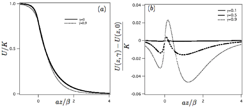
Figure 7: Comparison of the shape of the traveling wave solution (33) with and without diffusion. On the left, in (a), a front solution with $\gamma=0$ and one with $\gamma=0.9$ are depicted. On the right, in (b), $\Delta U(z,\gamma)=U(z,\gamma)-U(z,0)$ between Eq. (33) with $\gamma=0.1,0.5,0.9$ and the case with $\gamma=0$ are shown.

The parameter $\gamma$ is a measure of the relative diffusion in the system. In Fig. (7) we show how the front solution changes as diffusion increases. As in reaction diffusion equations, it is clear in Fig. (7b) that, as diffusion increases, the tail of $U(z,\gamma)$ acquires a shallower profile. The steepness of the tail as function of $\gamma$ can be determined from Eq. (33b). The front tails are sums of two exponentials each one with characteristic lengths ($\lambda_{2}$ and $\lambda_{3}$) and multiplicative weighing factors ($B_{2}$ and $B_{3}$), all functions of $\gamma$. When $\gamma=0$, $B_{2}=0$ and $\lambda_{2}=0$. Eq. (33b) then contains only one exponential term. The tail of the front solution is thus given by

$$U\left(az/\beta>0,0\right)=B_{3}\exp\left(-\frac{az}{\beta\lambda_{3}}\right)=\alpha\,K\,\exp\left(-az/\beta\right).$$ (35)

At the other extreme, i.e., when $\gamma=1$, the characteristic lengths $\lambda_{2}$ and $\lambda_{3}$ are equal to each other, the divergent part of the coefficients, $\xi$, cancels in the sum, and the tail of the front solution becomes

$$U\left(az/\beta>0,1\right)=(B_{2}+B_{3})\exp\left(-\frac{az}{\beta 2}\right)+=\alpha\,K\,\exp\left(-\frac{1}{2}az/\beta\right).$$ (36)

For values $0<\gamma<1$, both exponentials contribute to the tail shape but for small $\gamma$ values $B_{2}$ is negligible and $\lambda_{3}\gg\lambda_{2}$ therefore making the second exponential in (33b) dominate. This dependence is plotted in Fig. 8.

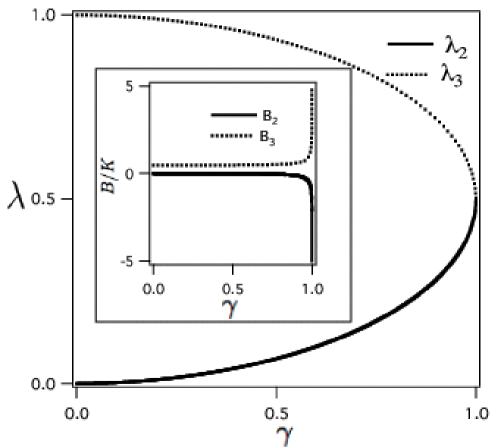
Figure 8: Plot of the dependence on $\gamma$ of the parameters associated with the traveling front solution (33b). The characteristic lengths of the exponentials $\lambda_{2}$ and $\lambda_{3}$ are depicted between the values $\gamma=0$ and $\gamma=1$. In the inset the multiplicative factors $B_{2}$ and $B_{3}$ are also plotted.

The use of the piecewise representation has allowed us to conduct an exact analysis above. When such a representation is not used, a perturbation scheme must be employed. The behavior shown in Fig. 8 lends support to the idea that a quantity directly related to $\gamma$ should serve as the small parameter on which to base the development of a perturbation technique for traveling front solutions. We develop such a scheme in the next subsection.

IV.2 Perturbation treatment for traveling fronts

The analysis presented here is a generalization of the technique proposed by Canosa canosa1973 for studying traveling fronts of the Fisher equation.

In the presence of diffusion, the traveling fronts of Eq. (31) are solutions of the following equation

$$\frac{\gamma^{2}}{4}U_{\zeta\zeta}+U_{\zeta}+Uf(U)=0,$$ (37)

where $\zeta=az/\beta$ and $z=x-ct$ where $c$ is the absolute speed of the traveling front.

The quantity $\xi=(\gamma/2)^{2}\leq 1/4$ is the perturbation parameter we will choose. A standard expansion of the traveling front in powers of $\xi$ in Eq. (31) gives the identity

$$U_{0}^{\prime}(\zeta)+\sum_{n=1}^{\infty}\xi^{n}\left(U_{n}^{\prime}(\zeta)+U_{n-1}^{\prime\prime}(\zeta)\right)+F\left[U_{0}+\sum_{n=1}^{\infty}\xi^{n}U_{n}\right]=0,$$ (38)

where $F(u)=uf(u)$. By Taylor-expanding the function $F(u)$, and rearranging each term in powers of $\xi$, it is possible to find the approximation of order $n$ in $\xi$ to the traveling front solution of Eq. (31). The zeroth order of such an expansion is given by the solution of

$$\frac{dU_{0}}{d\zeta}+F(U_{0})=0$$ (39)

which has been analyzed in the previous sections. The next order is given by

$$\frac{dU_{1}}{d\zeta}+\frac{d^{2}U_{0}}{d\zeta^{2}}+U_{1}F^{\prime}(U_{0})=0,$$ (40)

whose solution is murray

$$U_{1}(\zeta)=-U_{0}^{\prime}(\zeta)\ln\left(4\,|U_{0}^{\prime}(\zeta)|\right)$$ (41)

The next order, the second, is given by

$$\frac{dU_{2}}{d\zeta}+U_{2}F^{\prime}(U_{0})+\frac{d^{2}U_{1}}{d\zeta^{2}}+\frac{1}{2!}F^{\prime\prime}(U_{0})U_{1}^{2}=0$$ (42)

which is a linear equation for $U_{2}$, and all the other functions are given by solutions of the previous orders.

To arbitrary order $n$, we have

$$\frac{dU_{n}}{d\zeta}+\frac{d^{2}U_{n-1}}{d\zeta^{2}}+U_{n}F^{\prime}(U_{0})+h(\{U_{i<n}\})=0$$ (43)

where $h(\{U_{i<n}\}$ are the rest of the terms that come from the $n$th power of $\xi$.

Canosacanosa1973 and Murraymurray have provided up to to first order for the Fisher case. For the trigonometric nonlinearity with $f(u)$ given by (10) studied earlier in the present paper, application of this perturbation techniques gives for the first order correction

$$U_{1}(z)=\frac{1}{\pi}\textrm{sech}(az/\beta)\ln\left(\textrm{sech}(az/\beta)\right).$$ (44)

To further analyze the validity of the perturbation scheme, we use the exact expression for the traveling fronts of the piecewise linear function and compare it with the results obtained from the zeroth, first, and second order perturbation. Fig. 9 shows the differences between the solutions for two different values of the diffusion constant represented by $\gamma=0.1$ and $\gamma=0.9$. We see that, for small $az/\beta$, the lower orders are more accurate than the higher orders. In space this corresponds to that part of the front profile close to the value where $U(z)=1/2$. However, for the rest of the $az/\beta$ range, the higher orders in the perturbation get closer to the actual solution. It is worth noticing that, for $\gamma=0.9$, which represents a high value of diffusion, the error committed is still low. Perhaps unexpectedly, for low values of $az/\beta$, the lower orders are more accurate. The convergence of the orders is fast: for $\gamma=0.1$ the second order is just overlaped by the first order.

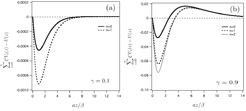
Figure 9: Difference between exact solution of the piecewise linear function and its zeroth, first and second order approximations in our perturbative treatment for two different values: $\gamma=0.1$ and $\gamma=0.9$ in (a) and (b) respectively. Notice that, although not shown in the graph, as the order of the perturbation increases the curve difference converges rapidly to a curve which represents the error upper bound.

The above analysis has uncovered a perhaps obvious but important point regarding the perturbation parameter. In (31), there are two characteristic velocities: the Fisher velocity $v_{f}=\sqrt{Da}$ and the medium velocity $v$. It may be tempting to suppose that the appropriate perturbation parameter is their ratio gk . This is not correct because the entire effect of the medium velocity $v$ can be eliminated by a transformation of the frame of reference. Our analysis above shows that it is crucial to take into consideration the third velocity that exists in the traveling wave context in this problem, viz. the velocity of the traveling wave $c$. The appropriate perturbation parameter when we consider a traveling wave is $v_{f}/(c-v)$ and our conclusion is that for diffusion to be considered as a perturbation on the pure convective analysis that we have presented in this paper, it is necessary that the velocity of the traveling wave exceed the medium velocity by an amount larger than the Fisher velocity.

V Summary

Several physically realizable situations exist in various areas of nonlinear population dynamics wherein the behavior is controlled primarily by the nonlinearities and the convective element of the motion, the diffusive contribution to the motion being small. The typical example is the behavior of bacteria in a petri dish nelson ; ana ; gk , where the so-called ”wind” motion induced by moving masks is made stronger than the inherent diffusive motion. A study of such situations has been provided in the present paper by first analyzing the case for no diffusion (sections II,III) and then extending the analysis to small diffusion (section IV). Explicit results have been obtained for a variety of nonlinearities on the basis of a straightforward prescription k , for the full initial value problem. Traveling waves have been analyzed explicitly for several cases. Interesting consequences such as the ”pyramid effect” for sinusoidal nonlinearities have been shown to occur. The effect of small diffusion has been incorporated through exact analysis for piecewise representation of the nonlinearities on the one hand and through perturbative calculations on the other.

- (1) R.A. Fisher, Ann. Eugen. 7, 355 (1937).
- (2) J.D. Murray, Mathematical Biology, 2nd edition (Springer, New York, 1993).
- (3) J.C. Skellam. Biometrika 38, 196 (1951)
- (4) V.M. Kenkre and M.N. Kuperman, Phys. Rev. E 67, 051921 (2003).
- (5) M. Ballard, V.M. Kenkre, and M.N. Kuperman, Phys. Rev. E 70, 031912 (2004)
- (6) G. Abramson and V.M. Kenkre, Phys. Rev. E 66, 011912 (2003).
- (7) G. Abramson, V.M. Kenkre, T. Yates, and R.R. Parmenter, Bull. Math. Bio. 65, 519 (2003).
- (8) V.M. Kenkre, in Modern Challenges in Statistical Mechanics: Patterns, Noise, and the Interplay of Nonlinearity and Complexity, V. M. Kenkre and K. Lindenberg, eds., AIP Proc. vol. 658 (2003), p. 63.
- (9) K.K. Manne, A.J. Hurd, and V.M. Kenkre, Phys. Rev. E 61, 4177 (2000).
- (10) G. Abramson, A.R. Bishop, and V.M. Kenkre, Phys. Rev. E 64, 66615 (2001).
- (11) M.A. Fuentes, M.N. Kuperman, and V.M. Kenkre, Phys. Rev. Lett. 91, 158104 (2003).
- (12) M.A. Fuentes, M. Kuperman, and V.M. Kenkre, J. Phys. Chem. B 108, 10505 (2004).
- (13) D.R. Nelson and N.M. Shnerb, Phys. Rev. E 58, 1383 (1998); K.A. Dahmen, D.R. Nelson, and N.M. Shnerb, J. Math. Biology 41, 1 (2000).
- (14) A.L. Lin, B.A. Mann, G. Torres-Oviedo, B. Lincoln, J. Kas, and H.L. Swinney, Biophys. J. 87, 75 (2004).
- (15) L. Giuggioli and V.M. Kenkre, Physica D 183, 245 (2003).
- (16) L. Giuggioli, Ph.D. Thesis (University of New Mexico).
- (17) V.M. Kenkre, Physica A 342, 242 (2004).
- (18) W.C. Allee, The Social Life of Animals, (Beacon Press, Boston,1938).
- (19) F. Courchamp, T. Clutton-Brock, and B. Grenfell, Trends Ecol. Evol. 14, 405 (1999).
- (20) P.A. Stephens and W.J. Sunderland, Trends Ecol. Evol. 14, 401 (1999).
- (21) C.W. Fowler and J.D. Baker, Rep. Int. Whaling Comm. 41, 545 (1999).
- (22) A. Rosas, C.P. Ferreira, and J.F. Fontanari, Phys. Rev. Lett. 89, 188101 (2001).
- (23) M. Remoissenet, Waves Called Solitons: Concepts and Experiments, 3rd edition, (Springer, Berliln, 1999).
- (24) Ed. M. Abramowitz and I.A. Stegun, Handbook of Mathematical Functions, (Dover, New York, 1970)
- (25) I.G. Petrovsky, Lectures on Partial Differential Equations, (Dover, New York, 1991)
- (26) G. Izus, R. Deza, C. Borzi, and H.S. Wio, Physica A 237, 135 (1997).
- (27) J. Canosa, IBM. J. Res. and Dev. 17 307 (1973).