ON THE GENEALOGY OF POPULATIONS: TREES, BRANCHES AND OFFSPRINGS

Abstract

We consider a neutral haploid population whose generations are not overlapping and whose size is large and constantly of $N$ individuals. Any generation is replaced by a new one and any individual has a single parent. We do not choose the stochastic rule which assigns the number of offsprings to any individual since results do not depend on the details of the dynamics, and, as a consequence, the model is parameter free. The genealogical tree is very complex, and distances between individuals (number of generations from the common ancestor) are distributed according to probability density which remains random in the thermodynamic limit (large population). We give a theoretical and numerical description of this distribution and we also consider the dynamical aspects of the problem describing the time evolution of the maximum and mean distances in a single population.

Pacs: 87.23.Kg, 05.40.-a

I 1. Introduction

In a population with asexual reproduction any individual has a single parent in previous generation. If the size of population is constant, some of the individuals may have the same parent and, therefore, the number of ancestors of present population decreases if one goes backward in time. At a finite past time one has complete coalescence and all population has a single ancestor. The genealogical distance between two individuals is simply the number of generations form the common ancestor. The resulting genealogical tree is very complex and has many branches, nevertheless, one would expect that in the limit of infinite population size, some quantities would reach some thermodynamic deterministic value. For example this could be the case for the frequency of genealogical distances in a single population or, at least, for the mean genealogical distance obtained considering all pairs of individuals. On the contrary, the frequency of distances in a single population is random even in the thermodynamic limit. This means that this frequency is different for different populations and also the mean distance obtained considering all pairs in a single population is random. This non self-averaging behavior is known since pioneering works of Derrida, Bessis and Peliti DB ; Derrida . In this paper we consider only the genealogical aspects of the problem, since mutation, at this level, is only a measure of genealogical distance through Hamming distance.

Let us define the model. We consider a population with asexual reproduction and whose generations are not overlapping in time. Any generation is replaced by a new one and any individual has a single parent. The size of the population is large and constantly of $N$ individuals, therefore, the average number of offspring of any individual is one. The stochastic rules which assign the number of offsprings to any individual can be chosen in many ways. In fact, results do not depend on the details of this rule, the only requirement is that the probability of having the same parent for two individuals must be of order $1/N$ for large $N$. As a consequence of the freedom in the choice of the rule, the model is parameter free. This is a typical situation if reproduction involves a fraction of order $N$ of the population. To be more clear we make two examples of stochastic dynamics which satisfy this assumption. First rule: at any generation one half of the individuals (chosen at random) has no offsprings and the remaining part has two (see Zhang ). With this rule the probability of having the same parent is $1/(N-1)$. The second rule (Wright-Fisher) is that any individual in the new generation chooses one parent at random in the previous one, independently on the choice of the others. In this case the probability of having the same parent for two individuals is exactly $1/N$.

In this paper we obtain analytical and numerical results. For numerical results we simulate a population of some hundred of individuals for $10^{7}$ generations according to Wright-Fisher rule. The population is large enough to avoid finite size corrections and time is sufficiently long to profit of ergodicity for substituting sample averages with time averages. Notice that we will use the world ’mean’ intending mean over different individuals of the same population and we will use ’average’ to intend average on many realization of the population process or, equivalently, by ergodicity, average on the same population at different times.

The relevant quantity is the random probability density (rpd) of pair distances in a single population. This quantity differs for different populations and changes in time for a single population. The aim of the paper is to obtain the statistics of this density and to obtain some informations about its dynamics. Section 2, 3, 4 and 5 are devoted to the first part of this program while section 6 is devoted to its dynamical aspects.

In the final section we point out the open problems and we discuss the possible relevance of results for the genealogy of mithocondrial DNA (mtDNA) populations.

II 2. distribution of pair distance

The genealogical tree of a population of $N$ individuals is determined by considering the set of all genetical distances between them. The distance between two given individuals is the number of generations from the common ancestor and since there are $N(N-1)/2$ possible pairs we have to specify $N(N-1)/2$ distances.

For large $N$ distances are proportional to $N$ so it is useful to re-scale them dividing by $N$. Equivalently we can say that distances are defined as the time from the common ancestor and contemporary define time as the number of generations divided by $N$.

Let us call $d(\alpha,\beta)$ the rescaled distance between individuals $\alpha$ and $\beta$ in the population. By definition if $\alpha$ and $\beta$ coincide the distance vanishes ($d(\alpha,\alpha)=0$). On the contrary, for two distinct individuals $\alpha$ and $\beta$ in the same generation one has

$$d(\alpha,\beta)=d(g(\alpha),g(\beta))+\frac{1}{N}\;\;,$$ (1)

where $g(\alpha)$ and $g(\beta)$ are the two parent individuals which coincide with probability $1/N$ and are distinct individuals $\alpha^{\prime}$ and $\beta^{\prime}$ with probability $(N-1)/N$. In other words, $d(\alpha,\beta)=1/N$ with probability $1/N$ and $d(\alpha,\beta)=d(\alpha^{\prime},\beta^{\prime})+1/N$ with probability $(N-1)/N$.

The above equation entirely defines the dynamics of the population, and simply state that the rescaled distance in the new generation increases by $1/N$ with respect to the parents distance. This dynamics can be easily simulated and at a given time (much larger than $N$ in order to forget initial conditions) it can be stopped. The distances obtained are different for different pairs and their frequency can be calculated. For finite $N$ frequency is simply the number of pairs in a given population with given distance $x$ divided by the total number $N(N-1)/2$ of possible pairs.

This frequency inside a single population of 500 individuals can be seen in Fig. 1. It is immediate to observe that this frequency is quite wild, due to the fact that individuals naturally cluster in subpopulation. In fact, most of the distances assume a few of values corresponding to the distances between the major subpopulations.

One could think that this singular behavior would disappear in the thermodynamic limit of large $N$. On the contrary, not only the singularity remains, but one easily realizes that this frequency remains random, being different for different populations and different for the same population at different times. Indeed, even the mean distance in a population and the largest distance in a populations are random quantities in the thermodynamic limit as we will see in the next section.

Let us stress again, that we use hereafter ’mean’ intending mean over different pairs of the same population and we use ’average’ to intend average on many realization of the population process or, equivalently by ergodicity, average on the same population at different times. Average will be indicated by $<\cdot>$.

In spite of the frequency we can consider the density $q(x)$

$$q(x)=\frac{2}{N(N-1)}\sum_{\alpha>\beta}\delta(x-d(\alpha,\beta))\,\,,$$ (2)

were the $\delta$ indicates the Dirac delta function.

This quantity is simply related to the frequency since $q(x)\,dx$ is the number of pairs whose distance lies in the interval $[x-\frac{dx}{2},x+\frac{dx}{2}]$ divided by the total number $N(N-1)/2$.

The random and singular nature of the density remains in the $N\to\infty$ limit and it is much the same of that of the overlap function in mean field spin glasses. In fact, both show similar non self-averaging properties. Indeed, the complete specification of the static properties of the model would be reached if one could be able to give the probability distribution of $q(x)$. We postpone this goal to section 5 and we only compute in this section the average of the density $<$$q(x)$$>$ and, in next two sections, the distribution of the largest distance (the distribution of the maximum of the support of $q(x)$ ) and the first two moments of the distribution of the mean distance.

Figure 1: Frequency $q(x)\,dx$ of distances in a single population. Here we compute this quantity for a population of $500$ individuals. Most of the distances assume a few of values corresponding to the distances between major subpopulations. Notice that this frequency is very different from its average $\exp(-x)\;dx$.

Let us now derive the average density $<$$q(x)$$>$. By using equation (1) and taking the average one has

$$<\exp(i\lambda\,d(\alpha,\beta))>\;=\;\frac{N-1}{N}\exp(\frac{i\lambda}{N})<\exp(i\lambda\,d(\alpha^{\prime},\beta^{\prime}))>\,+\,\frac{1}{N}\,\,.$$ (3)

Since the two expectation at the left and right side of the above equation (3) are equal, terms of order $1$ disappear and only terms of order $1/N$ must be retained. One gets

$$<\exp(i\lambda\,d(\alpha,\beta))>=\frac{1}{1-i\lambda}\,\,.$$ (4)

This result, which holds for large $N$, implies by Fourier inversion, that the average probability density for $d(\alpha,\beta)$ (i.e. $<$$\delta(x-d(\alpha,\beta))$$>$) is simply $\exp(-x)$. We remark that this is not the density of the distances inside a single large population but the average distribution of two individual distance sampled over many stochastically equivalent populations or, which is the same, sampled over the same population at many different times.

Notice that this result was already implicitly found in Derrida . In fact, in Derrida , the genetic overlap $o(\alpha,\beta)$ of two individuals is deterministically associated to the genealogical distance by $o(\alpha,\beta)=\exp(-d(\alpha,\beta)/\lambda)$ and the probability density for $o(\alpha,\beta)$ is given as $\lambda x^{\lambda-1}$ which is directly obtainable from the density $\exp(-x)$ for the distance. The deterministic relation between distance and overlap is due to the infinite genome limit and $\lambda$ is simply the inverse of the mutation rate. Let us mention that the Hamming distance is linearly associated to the overlap by $1-o(\alpha,\beta)$. In conclusion, one can easily understand that all the complex behavior of the genetic of the populations is due to the complexity of the structure of the genealogical tree, the role of mutation being simply accounted by the relations $o(\alpha,\beta)=\exp(-d(\alpha,\beta)/\lambda)$.

We are finally able to compute the average density using $<$$\delta(x-d(\alpha,\beta))$$>=\exp(-x)$. In fact, it is immediate

$$<q(x)>=\frac{2}{N(N-1)}\sum_{\alpha>\beta}<\delta(x-d(\alpha,\beta))>=\exp(-x)\,\,.$$ (5)

This smooth average density is completely different from a typical sample. To appreciate this fact is useful to look again at Fig. 1 were the frequency $q(x)\,dx$ is plotted. The most important consequences of this randomness will be discussed in the next section.

III 3. distribution of mean and maximum distances

Let us introduce now two quantities which sinthetically describe the “thermodynamic” state of a population.

The first is the mean distance

$$d=\frac{2}{N(N-1)}\sum_{\alpha>\beta}d(\alpha,\beta)\;\;,$$ (6)

which is simply the mean on a single population (and at a given time) of the internal distances considering all the $N(N-1)/2$ possible pairs. The above equation can be simply rewritten as $d=\int y\,q(y)\,dy$. Since the probability density $q(y)$ is random we expect that $d$ is also random.

The second quantity is the maximum distance

$$d_{max}\;=\;\max_{\{\alpha,\beta\}}\,d(\alpha,\beta)\;\;,$$ (7)

which is the largest distance in a single population, i.e. the maximum of the support of $q(y)$. Again, as a consequence of the randomness of the density $q(y)$ we expect that $d_{max}$ is also random. This quantity can be interpreted as the time from the common ancestor of the whole population and it has an evident relevance in paleontology. In fact, mtDNA of a single species is only transmitted by female and, therefore, can be considered as an haploid population. For what concerns Homo Sapiens, $d_{max}$ is the time from the celebrated mithocondrial Eve.

This two quantities can be studied in the context of the coalescence problem which has been widely investigated in a number of papers in the last two decades Ald ; Don ; King1 ; King2 ; King3 ; King4 ; Mohle1 ; Mohle2 ; Tavare ; Wat , and is still investigated in present times Avi ; Fill ; Goh ; Serva2 . We will come back to this approach in next two sections.

Both the distances $d$ and $d_{max}$ are random quantities even in the infinite population size limit and our goal is to find their density distributions $\rho(x)=<$$\delta(x-d)$$>$ and $\rho_{max}(x)=<$$\delta(x-d_{max})$$>$. We have computed them numerically, iterating the dynamics (1) for $10^{7}$ generations for a population of $N=100$ individuals. The results are shown in Fig. 2. where both the numerical densities are plotted.

The theoretical $\rho_{max}(x)$ will be obtained in next section for a thermodynamic ($N=\infty$) population and it is also plotted in Fig 1. Coincidence between numerical and theoretical density proves that $N=100$ can be already considered large.

On the contrary, we have not been able to deduce theoretically the density $\rho(x)$. Nevertheless, we compute its two first moments and we show how it can be done in principle and with a lot of work for higher moments. First notice that from (6) one has $<$$d$$>=<$$d(\alpha,\beta)$$>=1$. Also notice that in the thermodynamic limit, again from (6), one has $<$$d^{2}$$>=<$$d(\alpha,\beta)\,d(\gamma,\delta)$$>$ where $\alpha,\beta,\gamma$ and $\delta$ are all distinct. In fact, terms in which two or more individuals coincide are negligible since they give a contribution of order $1/N$ to $<$$d^{2}$$>$.

Figure 2: Probability density for the maximum distance (+) and for the mean distance ($\times$). The two densities are computed using a sample resulting from the dynamics of a population of $100$ individuals for $10^{7}$ generations. The full line corresponds to the theoretical probability density for the maximum distance ($N=\infty$). Since the empirical density corresponds to $100$ individuals only, we deduce that a population size of $100$ is sufficiently large to destroy finite size effects.

Then, we can use again equation (1) in order to compute the quantities $<$$d(\alpha,\beta)d(\beta,\gamma)$$>$. To reach this goal one simply has to take into account that any of the pairs which can be formed by two of the four individuals $\alpha$, $\beta$, $\gamma$ and $\delta$ may have coinciding parents with probability of order $1/N$. The probability that more then two parents coincide is of higher order and can be neglected. Then, with the same procedure which lead to (4), (terms of order 1 disappear and only those of order $1/N$ are retained) one finds

$$6<d(\alpha,\beta)d(\gamma,\delta)>=4<d(\alpha,\beta)d(\beta,\gamma)>+2<d(\alpha,\beta)>\,\,.$$ (8)

Again equation (1) can be used in order to compute the quantity $<d(\alpha,\beta)d(\beta,\gamma)>$ and obtain from terms of order $1/N$

$$3<d(\alpha,\beta)d(\beta,\gamma)>=<d^{2}(\alpha,\beta)>+2<d(\alpha,\beta)>\,\,.$$ (9)

Finally, from (4) not only one has $<$$d(\alpha,\beta)$$>=1$ but also $<$$d^{2}(\alpha,\beta)$$>=2$.

Solving this simple system of equations one gets $<$$d(\alpha,\beta)d(\beta,\gamma)$$>$=4/3 and $<$$d(\alpha,\beta)d(\gamma,\delta)$$>=11/9$ which implies $<$$d^{2}$$>$=$<$$d(\alpha,\beta)d(\gamma,\delta)$$>=11/9$. Summarizing:

$$<d>=1,\;\;\;\;\;<d^{2}>=\frac{11}{9}\;\;,$$ (10)

which coincide with the numerical values obtained from the string of $10^{7}$ generations. The above results are related to those in Derrida where analogous quantities are computed for the mean overlap of a population.

Let us finally mention, that higher moments can be computed using the same strategy. The result can be always found by solving a system of linear equations. The problem is that the number of equations in the system grows exponentially with the power of the moment.

IV 4. Coalescence

The content of this section is devoted to the most studied problem for this model: the coalescent. The idea is very simple and goes back to the papers of J. F. C. Kingman King1 ; King2 ; King3 ; King4 and some results has been also independently discovered in DB ; Derrida .

Consider a sample of $n$ individuals in a population of size $N$. The probability that they all have different parents in the previous generation is $\prod_{k=0}^{n-1}\,(1-\frac{k}{N})$. Therefore, the probability that their ancestors are still all different in a past time $t$ corresponding to $tN$ generations is $[\prod_{k=0}^{n-1}\,(1-\frac{k}{N})]^{tN}$. If $N$ is large compared to $n$ this quantity is approximately $\exp(-c_{n}t)$ where $c_{n}=\frac{n\,(n-1)}{2}$. Therefore, the average probability density for first coalescence is

$$p_{n}(t)=c_{n}\exp(-c_{n}t)\,\,.$$ (11)

This expression is the probability density for the first past time at which the ancestors of the $n$ individuals reduce to $n-1$. In particular, for $n=2$ one also re-obtain the probability density $\exp(-x)$ for the distance of a pair of individuals already found in section 2.

At the random time $\tau_{n}$ distributed according to the exponential of parameter $c_{n}$, the number of ancestor is $n-1$ and one has to go back an exponentially distributed time $\tau_{n-1}$ of parameter $c_{n-1}$ before further coalescence and so on. Therefore, the joint probability density $\prod_{k=m+1}^{n}\,p_{k}(t_{k})$ gives the statistics for successive coalescence times $\tau_{n}\,,\tau_{n-1}\,,...,\tau_{m+1}$ until the number of ancestor reduces to $m$. This is the core of the celebrated coalescent, which is mostly associated to the name of the probabilist J.F.G. Kingman.

If one wants to know the density distribution of time for $n$ individuals to coalescence to $m$ ancestor one simply has to compute the convolution of the $n-m$ successive exponentials. In other words this random time is simply the sum $\sum_{k=m+1}^{n}\,\tau_{k}$.

The computation of the time $d_{max}$ necessary for the ancestors of all individuals $N$ of a population to reduce to $m$ needs some care in dealing with limits since, in this case, $n=N$. Nevertheless, for large $N$, one easily obtains $d_{max}=\sum_{k=m+1}^{\infty}\tau_{k}$.

In order to compute explicitly the statistics for $d_{max}$ let us define $\rho_{n}(x)$ as the time density distribution of time for complete coalescence of $n$ individuals to a single ancestor. We have the convolution

$$\rho_{n}(x)=\;\int_{0}^{x}\,dt\,p_{n}(x)\;\rho_{n-1}(t-x)\,\,,$$ (12)

with the obvious $\rho_{2}(x)=p_{2}(x)=\exp(-x)$. Then, the density for $d_{max}$ is simply

$$\rho_{max}(x)=\lim_{n\to\infty}\rho_{n}(x)\,\,.$$ (13)

In Appendix 1 we compute explicitly the convolution (12) and we obtain the simple sum representation for the coalescent probability density $\rho_{n}(x)$:

$$\rho_{n}(x)=\sum_{l=2}^{n}\;\,(-1)^{l}\,(2l-1)\,c_{l}\;\left(\prod_{s=1}^{l-1}\frac{n-s}{n+s}\right)\exp\{-\;c_{l}\;x\}\,\,.$$ (14)

In the limit $n\to\infty$ one obtains the density for $d_{max}$

$$\rho_{max}(x)=\sum_{l=2}^{\infty}\;\,(-1)^{l}\,(2l-1)\,c_{l}\;\exp\{-\;c_{l}\;x\}\,\,.$$ (15)

This theoretical density (see also DB ; Derrida and very recently Fill ; Goh ) is plotted in Fig 2. where it is compared with the density obtained by the simulation of a population of 100 individuals. As already mentioned, the fact that they coincide so precisely can be considered further evidence that $N=100$ is sufficiently large that finite size effect are negligible.

Notice that this result is far from being complete, since it gives the distribution of the maximum distance $d_{max}$ of the support of $q(x)$ but it does not give more general informations on the distribution of the density $q(x)$ itself. This problem will be faced in next section.

Before ending this section we would like to complete the description of the coalescent process by considering the number of offsprings of any of the ancestors. Suppose that the total number of individuals in present generation is $N$, then, any of the $m$ ancestors has, in present generation, a number $\eta_{i}^{m}\,N$ of offsprings (with $i=1,2,...,m$ and with $\sum_{i=1}^{m}\eta_{i}^{m}=1$). Successive coalescence reduces the number of ancestors to $m-1$ and one has that any of them has $\eta_{i}^{m-1}\,N$ offsprings in present population ($\sum_{i=1}^{m-1}\eta_{i}^{m-1}=1$). These last numbers are such that $m-2$ of them are the same of the $\eta_{i}^{m}$ and one is the sum of the two remaining of the $\eta_{i}^{k}$, correspondingly to the pair which have matched in a single ancestor. This rule can be iterated until the number of ancestors reduces to a single one.

Therefore, the coalescent picture is completed by considering this random rule which permits to obtain the $\eta_{1}^{m-1},....\eta_{m-1}^{m-1}$ from the $\eta_{1}^{n},....\eta_{m}^{n}$ for any $m<n$. The rule being simply that at any step two of the numbers are chosen at random and summed, while the others are left unchanged. Notice that this part of the coalescent process is independent form the random times $\tau_{1},\,\tau_{2},\,...\tau_{n}$.

V 5. statistics of the random density

We have seen that the time one has to go backward in order that the ancestors of all $N$ individuals of a population reduces to $m$ is $q_{m+1}=\sum_{k=m+1}^{\infty}\tau_{l}$. In this case, any of the $m$ individuals will be the ancestor of a number $\eta_{i}^{m}\,N$ of individuals ($i=1,2,...,m$) with $\sum_{i=1}^{m}\eta_{i}^{m}=1$. In other words, any of the $m$ ancestor will be at the basis of a branch with a number $\eta_{i}^{m}\,N$ of final offsprings. Successive coalescence reduces the number of ancestors to $m-1$, which means the branches of two of the $m$ ancestors are now sub-branches of a single one.

We can now easily see how distances are distributed in a population. At a past time $q_{2}$ we have that the last two common ancestors, any of them with a number of final offsprings $\eta_{1}^{2}$ and $\eta_{2}^{2}$ match in a single ancestor. Therefore, there are $(\eta_{1}^{2}\,N\,)\,(\eta_{2}^{2}\,N)$ pairs whose distance is $q_{2}$ which means that the fraction of pairs whose distance is $q_{2}$ is $p_{2}=2\eta_{1}^{2}\,\eta_{2}^{2}$ according to the fact that the total number of pairs is $N(N-1)/2$.

At a past time $q_{3}$ we have that two of the last three common ancestors match in a single ancestor. Their final offsprings before matching are $\eta_{1}^{3}$, $\eta_{2}^{3}$ and $\eta_{3}^{3}$. One of these three numbers equals $\eta_{1}^{2}$ or $\eta_{2}^{2}$ and the sum of the other two (say $\eta_{i}^{3}$ and $\eta_{j}^{3}$) equals the remaining one of $\eta_{1}^{2}$ and $\eta_{2}^{2}$. The fraction of pairs whose distance is $q_{3}$ is $p_{3}=2\eta_{i}^{3}\,\eta_{j}^{3}$.

Then we go on and at time $q_{m}$ we have that two of the last $m$ common ancestors match in a single one. The numbers of their offsprings before matching are $\eta_{1}^{m},\,\eta_{2}^{m},\,....\,\eta_{m}^{m}$. There are $m-2$ of these numbers which equal $m-2$ of the $\eta_{1}^{m-1},\,\eta_{2}^{m-1}2,\,....,\,\eta_{m-1}^{m-1}2$ and two (say $\eta_{i}^{m}$ and $\eta_{j}^{m}$) whose sum equals the remaining one. The fraction of pairs whose distance is $q_{m}$ is $p_{3}=2\eta_{i}^{m}\,\eta_{j}^{m}$.

It is now quite clear how the probability density $q(x)$ looks like. First, its support is only in the random times $q_{k}$ with $2\leq k<\infty$ and where $q_{k}=\sum_{l=k}^{\infty}\tau_{l}$. Second, the fraction of pairs corresponding to distances $q_{1},q_{2}...$ is $p_{1},p_{2},...$ which satisfy $\sum_{k=1}^{\infty}p_{k}=1$.

Therefore, the probability density $q(x)$ is

$$q(x)=\sum_{l=2}^{\infty}p_{l}\delta(x-q_{l})\,\,.$$ (16)

Now, what we need is to give the statistics of the numbers $q_{2},q_{3},...$ and $p_{2},p_{3},...$.

The first part of this program is simple. In fact, since the probability for the sequence $\tau_{2},\tau_{3},...$ is $\prod_{k=2}^{\infty}\,c_{k}\,\exp(-\,c_{k}\,t_{k})$ and since $q_{l+1}=q_{l}-\tau_{l}$ we have that joint probability for the sequence $q_{2},q_{3},...$ is

$$\prod_{k=2}^{\infty}\,c_{k}\,\exp[-\,(k-1)\,q_{k}]\,\,,$$ (17)

where it is assumed that $q_{k}\geq q_{k+1}$.

The second part of the program is a little more difficult. First we stress that $\tau_{2},\tau_{3},...$ are independent from the sizes $\eta_{i}^{j}$ and, therefore, the the random sequence $p_{2},p_{3},...$ is independent from the sequence $q_{2},q_{3},...$ .

To obtain the statistics for $p_{2},p_{3},...$ we have to consider the coalescence rule for the $\eta_{i}^{j}$ described at the end of previous section. According to it, one has the conditional probability $p(\eta_{1}^{m-1},....,\eta_{m-1}^{m-1}\,|\,\eta_{1}^{m},....,\eta_{m}^{m})$ which is constant whenever the rule is satisfied and vanishes elsewhere.

Assume that the limit of infinite $N$ holds, in this case the numbers $\eta_{1}^{m},\,....\,\eta_{m}^{m}$ may assume any real value on $\sum_{i=1}^{m}\,\eta_{i}^{m}=1$. Also assume that the probability density $q(\eta_{1}^{m},....,\eta_{m}^{m})$ is constant on $\sum_{i=1}^{m}\eta_{i}^{m}=1$ and vanishing elsewhere. Than, the probability density for the $q(\eta_{1}^{m-1},....,\eta_{m-1}^{m-1})$ is also constant on $\sum_{i=1}^{m-1}\eta_{i}^{m-1}=1$ and vanishing elsewhere. This property can be easily verified using the above described conditional probability density (see also King1 ).

Therefore, if the probability density $q(\eta_{1}^{n},....,\eta_{n}^{n})$ is constant for a given $n$ then it is constant for any $m\leq n$ and the process rule can be easily reversed. In other words, the conditional probability $p(\eta_{1}^{m},....,\eta_{m}^{m}\,|\,\eta_{1}^{m-1},....,\eta_{m-1}^{m-1})$ can be computed from $p(\eta_{1}^{m-1},....,\eta_{m-1}^{m-1}\,|\,\eta_{1}^{m},....,\eta_{m}^{m})$ and $q(\eta_{1}^{m},....,\eta_{m}^{m})$ . The only point which need some care is to show that for infinite $N$ the density $q(\eta_{1}^{n},....,\eta_{l}^{n})$ is, indeed, constant for a given $n$ . This task is accomplished in Appendix 2.

Using the above results we obtain with a simple calculation that the conditional density $p(\eta_{1}^{m},....,\eta_{m}^{m}\,|\,\eta_{1}^{m-1},....,\eta_{m-1}^{m-1})$ corresponds to the following reversed rule: one chooses at random $1\leq i\leq m-1$ with probability $\eta_{i}^{m-1}$ and cut $\eta_{i}^{m-1}$ in two segments $\chi\eta_{i}^{m-1}$ and $(1-\chi)\eta_{i}^{m-1}$ with $\chi$ uniformly distributed between 0 and 1. Then one has that two of the $\eta_{1}^{m},....,\eta_{m}^{m}$ are $\chi\eta_{i}^{m-1}$ and $(1-\chi)\eta_{i}^{m-1}$ while the others $m-2$ equals the remaining $m-2$ of the $\eta_{1}^{m-1},....,\eta_{m-1}^{m-1}$.

There is a picture that is useful to shortly describe the rule. Consider a square with unitary surface. Choose a point $x_{2}$ with uniform distribution between 0 and 1. Put it on the basis of the square, then it will cut the unitary segments in two parts which can be identified with $\eta_{1}^{2}$ and $\eta_{2}^{2}$. Therefore, the shaded area in Fig 3a is $p_{2}$. Then choose a second point $x_{3}$ with uniform distribution between 0 and 1. Put it on the basis and it will be in one of the two previously created segments with probability proportional to their size. Furthermore, the cut in the chosen segment will be uniformly distributed on it. Then, $p_{3}$ will be the darker shaded area of Fig 3b. Then choose a third point $x_{4}$ with uniform distribution between 0 and 1. Put it on the basis of the square and it will be in one of the three previously created segments with probability proportional to the their size. Furthermore, the cut in the chosen segment will be uniformly distributed on it. Then $p_{4}$ will be the darkest shaded area of Fig 3c. Then you can go on and the whole square will be shaded when the operation is repeated infinite times.

In conclusion, we have the complete rule for constructing $q(x)$ since we have the joint probability for $q_{2},\,,q_{3},\,....$ and we have the simple rule exemplified in Fig. 3 for the joint probability for $p_{2},\,p_{3},\,....$ .

Indeed, we are not able to find explicitly this second joint probability density and, at this stage, the result is little more than transforming a complicate random dynamics (1) in a simpler random rule of repeated fractioning.

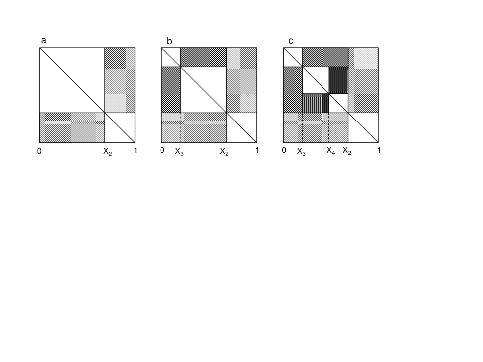
Figure 3: The point $x_{2}$ is chosen with uniform distribution on [0, 1] than the shaded area in (a) is $p_{2}$. The point $x_{3}$ is also chosen with uniform distribution on [0, 1], then, $p_{3}$ is the darker shaded area in (b). The point $x_{4}$ is also chosen with uniform distribution on [0, 1], then, $p_{4}$ will be the darkest shaded area in (c). The whole square will be shaded when the operation is repeated infinite times correspondingly to the fact that $\sum_{i=2}^{\infty}p_{i}=1$.

Before ending this section we would like to make some comments. Notice that the average value of $d_{max}$ ($d_{max}$ is $q_{2}$) is $<$$d_{max}$$>=2$, which means that a population has a common ancestor at a past time which corresponds in average to $2N$ generations. On the other side, the time for the number of ancestors to reduce to two is $q_{3}$ with $<$$q_{3}$$>=1$. Therefore, the number of generation one has to step backward in order that ancestors reduce to a pair is $N$ in average and, then, it is necessary to step backward $N$ more generation in average before ancestors reduce to a single. This also means that for any realization of the process, the density $q(x)$ has an isolated Dirac delta corresponding to the maximum distance while all the remaining support is concentrated in a segment whose size is, in average, one half of the maximum distance.

This means that any population naturally splits in two subpopulation which are the descendants of two different ancestors. All the distance between pair of individuals from the two different subpopulation coincide with the maximum distance $d_{max}$ of average 2, on the contrary, the distances inside the two subpopulations are in average smaller than 1. This considerations will find a motivation in the final discussion.

VI 6. Dynamics

The dynamics of the model is in principle very complicated, since one should be able to describe the time evolution of the density $q(x)$. As a more reachable goal one could try to describe the time evolution of the maximum distance and of the mean distance in a population. The behavior of these quantities is shown in Fig.4 where we plot the maximum distance and mean distance of the individuals of a single population as a function of time. The two distances result from the dynamics of a population of $N=500$ individuals generated for $5000$ generations which correspond to a time lag $10$. Notice that both distances are subject to abrupt negative variations due to the extinction of large subpopulations. In particular the maximum distance increases constantly until has a large negative jump due to the extinction of one of the two subpopulations which are composed by the offsprings of one of the last two ancestors of the whole population. At this point one of the other ancestor become the last common ancestor of all population and the maximum distance is reduced consequently.

Figure 4: Maximum distance (full line) and and mean distance (slashed line) of the individuals of a single population as a function progressive generation number. The two distances result from the dynamics of a population of $N=500$ individuals generated for $5000$ generations (time is number of generations divided by $N$). The size of the population is sufficiently large to destroy finite size effects. Notice that both distances are subject to abrupt negative variations due to the extinction of large subpopulations.

The full line in Fig. 4 gives the maximum distances at all times, while the maximum distances at the time of jumps correspond to its relative maxima. Furthermore, the jump sizes are the differences between relative maxima and subsequent relative minima of the same full line.

How are distributed jumps and relative maxima? In order to compute the densities of these two quantities we have generated a dynamics for a population of $100$ individuals for $10^{7}$ generations corresponding to about of $10^{5}$ relative maxima. Both densities are plotted in Fig. 5.

The probability density for the size of jumps, shown in Fig. 5, is compatible with $\exp(-x)$ which is quite surprising. In fact, it is true that the density of distance between the last two ancestors is $\exp(-x)$, but, this is true in average with respect a generic time, and not necessarily at the times of jumps. Even more surprising is that the empirical density of the maximum distance at the times of jumps coincides (Fig. 5) with the theoretical density (15). The second, in fact, gives the statistics of the maximum density at a generic time. In other words, the first is the density of the relative maxima of the full line in Fig. 4, while the second is the density of all the points of the same full line.

Figure 5: In this picture we have the probability density of the maximum distance (+) at the time of jumps and the probability density for the size of jumps ($\times$). The maximum distances at the time of jumps correspond to the relative maxima of the maximum distance process (see Fig. 4). These densities ($100$ individuals) are computed from a sample of $10^{5}$ maxima. Comparison with the full line (the theoretical probability density for the maximum distance) shows that the statistical properties of the maximum distance and of the maximum distance at the times of jumps are the same. The probability density for the size of jumps ($\times$) is compared with $\exp(-x)$.

Finally, we would find the statistics for the lags between jumps. Again, in order to compute this density we have generated a dynamics (1) for a population of $100$ individuals for $10^{7}$ generations corresponding to about $10^{5}$ lags. The result, as it can be seen in Fig. 6, is that lags between jumps are exponentially distributed according to $\exp(-x)$.

In order to understand this behavior is sufficient to consider that the time of jumps is when one of the two subpopulation corresponding to the two more recent ancestors of all individual extinguish. Assume that at a given time $t$ the number of the individuals belonging to the two subpopulations is $yN$ and $(1-y)N$, then at the next generation (at time $t+1/N$) this numbers are $zN$ and $(1-z)N$. Assuming Wrigh-Fisher rule we have that the probability density for $z$ given $y$ is

$$\rho(z\;|\;y)=\left(\begin{array}[]{cc}N\\ Nz\end{array}\right)\;y^{Nz}\;(1-y)^{N(1-z)}\,\,,$$ (18)

which in particular implies the two following conditional expectations for $z$ and $z^{2}$ given $y$:

$$<(z\;|\;y)>=y\;\;\;\;\;\;<(z^{2}\;|\;y)>=y^{2}+\frac{y\,(1-y)}{N}\,\,.$$ (19)

It is now simple to construct the diffusion limit of (18). In fact, if we write $x(t+\frac{1}{N})=z$ and $x(t)=y$ we have $<x(t+\frac{1}{N})-x(t)>=0$ and $<(x(t+\frac{1}{N})-x(t))^{2}>=\frac{x(t)\,(1-x(t))}{N}$ which can be written in the continuous time limit as

$$dx(t)=\sqrt{x(t)\,(1-x(t))}\;dw(t)\,\,,$$ (20)

where $w(t)$ is the Brownian motion (see also Don ).

All what we need now to compute the statistics of the lags between extinctions (which are the lags between jumps) is to compute the statistic of the hitting times for this process at the frontier $z=0,\;z=1$. After the process reaches the frontier a new process starts at a point which is uniformly distributed between 0 and 1. This choice depends on the known fact that the two main branches of the subpopulation which have survived have a size uniformly distributed.

Indeed, the statistic is simply exponential. In order to show this fact we have simulated the above equation for a time sufficient to have $10^{5}$ extintions (hitting times). The resulting probability density is shown in Fig. 6. were it is also plotted the same density as it results from (1).

Figure 6: Probability density for the lag between jumps computed from the generated dynamics of $100$ individuals ($\times$) and probability density of lags between jumps computed from the simulation of the exit time for the Wiener process (+). The two densities are both obtained from a sample of $10^{5}$ lags and both coincide with the exponential density $\exp(-x)$.

VII 7. Discussion

Before discussing the open problems concerning the model in this paper, we would like to comment eventual relevance of its complex phenomenology for biological applications. Our example concerns the use of mtDna in recent paleoanthropological studies. What makes mtDNA interesting is that it is inherited only from the mother and it reproduces asexually at variance with nuclear DNA, therefore, results in this paper should apply to it. In this sense, mtDNA of a given species which should be considers as an haploid population. Furthermore, assuming that mtDNA mutates at a constant rate, the number of differences in mtDNA between two individuals is a measure of their genealogical distance in maternal lineage. Let us illustrate our example.

In the years from 1997 to 2000 some mtDNA from three different specimen of Neandertal was extracted Krings1997 ; Krings2000 and short strands of the hyper-variable region (HVR1 and HVR2) were amplified using Polymerase Chain Reaction (PCR).

Two different mtDNA sequences were extracted from the first specimen. For the first sequence modern humans differed from each other in 8.0 $\pm$3.1 positions, while the Neandertals differed in 27.0 $\pm$2.2 positions from modern humans. For the second mtDNA sequence modern humans differed from each other by 10.9 $\pm$5.1 and the Neandertals differed in 35.3 $\pm$2.3 from modern humans. The mtDNA sequence of the second Neandertal was compared with a particular modern human sequence, known as the reference sequence. Difference from reference modern human sequence was in 22 position, (27 for the first Neandertal) while the two Neandertals differed from each other in 12 positions. Sequencing of a third Neandertal mtDNA confirmed previous result since the difference from modern humans was in 34.9 $\pm$ 2.4 positions.

The conclusion was that, given the above ranges in differences, the Neandertals mtDNA is statistically different from modern humans mtDNA. We think that this conclusion is doubtful since results and discussion in section 5 show that this situation is absolutely typical. This fact can be also appreciated in Fig. 1.

Let us continue with our example. A modern human fossil, 60,000 years-old, (older then the three Neandertal fossils) was discovered in 1974 in the dry bed of Lake Mungo in Australia. Recently, some sequences of his mtDNA were extracted from fragments of his skeleton Adcock and from differences between Mungo mtDNA and living aborigines mtDNA and conclude that Mungo man belongs to a lineage diverging before the most recent common ancestor of contemporary humans. Also in this case, the argument is doubtful, in fact, rapid extinctions of mtDNA subpopulations at all scales are well evident in Fig. 4.

The conclusion was that both Neandertals and Mungo man should be eliminated from our ancestry. It was argued, in fact, that the distance of Neandertals from living humans was too large and that Mungo carried a mtDNA which disappeared from modern humanity. On the contrary, it is possible that this is not true since one can observe this mtDNA phenomenology in a perfectly inter-breeding and (nuclear DNA) homogeneous population. In fact, sexually reproducing nuclear DNA has a completely different statistics JM ; DMZ ; Serva and in large populations the distance for almost all pairs of individuals coincide with the average value Serva .

We would like to conclude by a list of open problems. First of all we would like to compute the probability density for the mean distance $d$. We are in principle able to painfully compute all moments of the random variable $d$ following calculations in section 3 but we are not able at the moment to give an explicit expression of its probability density. More important, we would like to find the explicit joint probability for $p_{2},\,p_{3},\,....$. Notice that we are able to give this probability only indirectly by the processes in paint-boxes of Fig. 3. Finally, we would like to characterize the time behavior of the maximum distance, which means to find the process for $d_{max}$ of which we have a realization in Fig. 4.

VIII Appendix 1

We give here a very simple derivation of an explicit representation for $\rho_{n}(x)$. We first show that

$$\rho_{n}(x)=\left(\prod_{s=2}^{n}c_{s}\right)\sum_{l=2}^{n}\left(\prod_{s=2;s\neq l}^{n}\frac{1}{c_{s}-c_{l}}\right)\exp(-c_{l}x)\,\,.$$ (21)

It can be directly verified that the above equation holds for $n=3$ according to (11) and (12). Furthermore, assuming that it holds for a given $n-1$, from (11) and (12) we obtain

$$\rho_{n}(x)=\left(\prod_{s=2}^{n}c_{s}\right)\sum_{l=2}^{n-1}\left(\prod_{s=2;s\neq l}^{n}\frac{1}{c_{s}-c_{l}}\right)\exp(-c_{l}x)-\left(\prod_{s=2}^{n}c_{s}\right)\sum_{l=2}^{n-1}\left(\prod_{s=2;s\neq l}^{n}\frac{1}{c_{s}-c_{l}}\right)\exp(-c_{n}x)\,\,.$$ (22)

If we compare (21) and (22) we see that they coincide provided

$$-\left(\prod_{s=2}^{n}c_{s}\right)\left(\prod_{s=2;s\neq n}^{n}\frac{1}{c_{s}-c_{n}}\right)\exp(-c_{n}x)-\left(\prod_{s=2}^{n}c_{s}\right)\sum_{l=2}^{n-1}\left(\prod_{s=2;s\neq l}^{n}\frac{1}{c_{s}-c_{l}}\right)\exp(-c_{n}x)=0\,\,,$$ (23)

which holds assumed that

$$\sum_{l=2}^{n}\left(\prod_{s=2;s\neq l}^{n}\frac{1}{c_{s}-c_{l}}\right)=0\,\,.$$ (24)

Therefore, all what we need to prove the preliminary representation (21) is that (24) holds. To reach this goal let us define the Lagrange polynomial

$$Q(x)=\sum_{l=2}^{n}c_{l}\left(\prod_{s=2;s\neq l}^{n}\frac{c_{s}-x}{c_{s}-c_{l}}\right)\,\,.$$ (25)

It is immediate to verify that for every $l$ such that $2\leq l\leq n$ one has $Q(c_{l})=c_{l}$. Since the degree of the polynomial is at most $n-2$ and since it crosses the above $n-1$ points it is necessarily $Q(x)=x$ and in particular $Q(0)=0$ Then, since by definition

$$Q(0)=\sum_{l=2}^{n}c_{l}\left(\prod_{s=2;s\neq l}^{n}\frac{c_{s}}{c_{s}-c_{l}}\right)=\left(\prod_{s=2}^{n}c_{s}\right)\sum_{l=2}^{n}\left(\prod_{s=2;s\neq l}^{n}\frac{1}{c_{s}-c_{l}}\right)\,\,,$$ (26)

equation (24) holds and (21) is demonstrated.

Furthermore, by a simple calculation one can show that

$$\left(\prod_{s=2}^{n}c_{s}\right)\sum_{l=2}^{n}\left(\prod_{s=2;s\neq l}^{n}\frac{1}{c_{s}-c_{l}}\right)=\,(-1)^{l}\,(2l-1)\,c_{l}\prod_{s=1}^{l-1}\frac{n-s}{n+s}\,\,,$$ (27)

and finally we have the simple sum representation for the coalescent density distribution

$$\rho_{n}(x)=\sum_{l=2}^{n}\;\,(-1)^{l}\,(2l-1)\,c_{l}\;\left(\prod_{s=1}^{l-1}\frac{n-s}{n+s}\right)\exp\{-\;c_{l}\;x\}\,\,.$$ (28)

IX Appendix 2

We show here that the probability density $q(\eta_{1}^{n},....,\eta_{l}^{n})$ is constant for a given $n$ when the limit of large $N$ is performed.

At a given time in the past, the number of ancestors of all $N$ individuals of a population is $l$. At an intermediate time, always in the past, the number of ancestors is $k\geq l$. This means that any of the $l$ individuals is an ancestor of one ore more of the $k$ individuals i.e., any of the $l$ branches has one or more sub-branches. Let us call $r_{i}^{l}$ this (integer) number of sub-branches for individual $i$, then, $\sum_{i=1}^{l}\,r_{i}^{l}=k$ with $r_{i}^{l}\geq 1$. Let us call $\Gamma_{l}$ the ensemble of $r_{1}^{l},\,.......\,r_{l}^{l}$ such that $\sum_{i=1}^{l}\,r_{i}^{l}=k$ and $r_{i}^{l}\geq 1$.

Let us define $f_{l}(r_{1}^{l},\,...\,r_{l}^{l})$ as the probability for $r_{1}^{l},\,...\,r_{l}^{l}$. We first show that this probability is constant on $\Gamma_{l}$ for any $l\leq k$.

Assume that $f_{l+1}(r_{1}^{l+1},\,...\,r_{l+1}^{l+1})$ is constant on $\Gamma_{l+1}$. Coalescence implies that one of $r_{1}^{l},\,...\,r_{l}^{l}$ equals the sum of two random chosen of the $r_{1}^{l+1},\,...\,r_{l+1}^{l+1}$ while the remaining $l-1$ coincides. Then, according to this rule, $f_{l}(r_{1}^{l},\,...\,r_{l}^{l})$ is constant on $\Gamma_{l}$. To have the proof, it is now sufficint to remark that $f_{k}(r_{1}^{k},\,...\,r_{k}^{k})$ is constant on $\Gamma_{k}$. In fact, all $r_{i}^{k}$ must equal one, i.e. $f_{k}(1,\,...\,1)=1$ while it vanishes elsewere.

Now, let us recall that the the number of offspring of the $k$ ancestors are $\eta_{1}^{k}\,N,\,....,\eta_{k}^{k}\,N$ with $\sum_{i=1}^{k}\eta_{i}^{k}=1$. Assume now that a previous time the number of ancestors is $n<k$ and assume that the number of sub-brances of any of them is $r_{1}^{n},\,...\,r_{n}^{n}$. Then, the numbers $\eta_{i}^{n}$ will be obtained by the sum of $r_{i}^{n}$ of the $\eta_{1}^{k}\,,....,\eta_{k}^{k}$ chosen at random.

Now let us recall that $\sum_{i=1}^{n}\,r_{i}^{n}=k$, therefore, large $k$ implies that for almost all possible choices on $\Gamma_{n}$ the $n$ numbers $r_{i}^{n}$ must be of order $k$. We can define $r_{i}^{n}=\alpha_{i}^{n}\,k$ with $\sum_{i=1}^{n}\,\alpha_{i}^{n}\,=1$ and the numbers $0\leq\alpha_{i}^{n}\leq 1$ of order 1. Furthermore, since $\sum_{i=1}^{k}\eta_{i}^{k}=1$, we assume that almost all of the $\eta_{i}^{k}$ are of order $1/k$.

We can now take the limit of large $k$ after the limit of large $N$. Since the $\eta_{i}^{n}$ are the sum of $r_{i}^{n}=\alpha_{i}^{n}\,k$ of the $\eta_{1}^{k}\,,....,\eta_{k}^{k}$ and since from definition $\sum_{i=1}^{k}\eta_{i}^{k}=1$ with $\eta_{i}^{k}$ of order $1/k$, one has $\eta_{i}^{n}=\lim_{k\to\infty}\,r_{i}^{n}\,/k=\alpha_{i}^{n}$.

Finally, since $f_{l}(r_{1}^{n},\,...\,r_{n}^{n})$ is constant on $\Gamma_{n}$ one has that $q(\eta_{1}^{n},....,\eta_{n}^{n})$ is constant on $\sum_{i=1}^{n}\eta_{i}^{n}=1$.

X Acknowledgements

We thank Davide Gabrielli, Michele Pasquini and Filippo Petroni for many illuminating discussions. We acknowledge the financial support of MIUR Universita’ di L’Aquila, Cofin 2004 n. 2004028108$\_$005.

References

- (1) G. Adcock, E. Dennis, S. Easteal, G. Huttley, L. Jermin, W. Peacock and A. Thorne, Mitochondrial DNA sequences in ancient Australians: Implications formodern human origins, Proceedings of the National Academy of Science 98, (2001), 537-542.
- (2) D. Aldous, Deterministic and Stochastic Models for Coalescence (Aggregation, Coagulation): a Review of Mean Field Theory for Probabilists, Bernoulli, 5, (1999), 3-48.
- (3) A. Dalal and E. Schmutz, Compositions of Random Functions on a Finite Set, Electronic Journal of Combinatorics, 9, R26, (2002).
- (4) B. Derrida and D. Bessis, Statistical properties of valleys in the annealed random map model, Jourmal of Physics A: Mathematical and General, 21, (1999), L509-L515.
- (5) B. Derrida and B. Jung-Muller, The genealogical tree of a chromosome, Journal of Statistical Physics, 94, (1999), 277-298.
- (6) B. Derrida, S. C. Manrubia and D. H. Zanette, Statistical properties of genealogical trees, Physical Review Letters, 82, (1999), 1987-1990.
- (7) B. Derrida and L. Peliti, Evolution in a flat fitness landscape, Bulletin of Mathematical Biology 53, (1991), 355-382.
- (8) P. Donnelly, Weak convergence to a Markov chain with an entrance boundary: ancestral processes in population genetics, The Annals of Probability, 19 No.3, (1991), 1102-1117.
- (9) J. Fill, On Compositions of Random Functions on a Finite Set, Preprint.
- (10) W. M. Y. Goh, P. Hitczenko and E. Schmutz, Iterating Random Functions on a Finite Set, ArXiv:math.CO/0207276v2, (2002).
- (11) J. F. C. Kingman, The Coalescent, Stochastic Processes and their Applications, 13, (1982), 235-248.
- (12) J. F. C. Kingman, On the genealogy of large populations. Essays in statistical science, Journal of Applied Probability, 19A, (1982), 27-43.
- (13) J. F. C.Kingman, Exchangeability and the evolution of large populations, in Exchangeability in probability and statistics, pp. 97-112, North-Holland, Amsterdam-New York, 1982.
- (14) J. F. C. Kingman, Mathematics of genetic diversity, CBMS-NSF Regional Conference Series in Applied Mathematics, 34. Society for Industrial and Applied Mathematics (SIAM), Philadelphia, Pa., 1980. ISBN: 0-89871-166-5.
- (15) M. Krings, C. Capelli, F. Tschentscher, H. Geisert, S. Meyer, A. von Haeseler, K. Grossshmidt, G. Possnert, M. Paunovic and S. P bo, A view of Neandertal genetic diversity, Nature Genetics, 26, (2000), 144-146.
- (16) M. Krings, A. Stone, R. W. Schmitz, H. Krainitzki, M. Stoneking and S. P bo, Neandertal DNA sequences and the origin of modern humans, Cell, 90, (1997), 19-30.
- (17) M. Möhle, Total variation distances and ratesof convergence for ancestral coalescenct processes in exchangeable population models, Advances in Applied Probability, 32, (2000), 983-993.
- (18) M. Möhle, Weak convergence to the coalescentin neutral population models, Journal of Applied Probability, 36, (1999), 446-460.
- (19) M. Serva, Lack of self averaging in family trees. Physica A 332, (2004), 387-393
- (20) M. Serva and L. Peliti, A statistical model of an evolving population with sexual reproduction, Journal of Physics A: Mathematical and General 24, (1991), L705-L709.
- (21) S. Tavare, Line-of-descent and geneological processes and their applications in population genetics models, Theoretical Population Biology, 26, (1984), 119-164.
- (22) G. A. Watterson, Lines of descent and the Coalescent, Theoretical Population Biology, 26, (1984), 256-276.
- (23) Y.-C. Zhang, M. Serva and M. Policarpov, Diffusion reproduction processes, Journal of Statistical Physics 58, (1990), 849-861.