Abstract

Prediction of one-dimensional protein structures such as secondary structures and contact numbers is useful for the three-dimensional structure prediction and important for the understanding of sequence-structure relationship. Here we present a new machine-learning method, critical random networks (CRNs), for predicting one-dimensional structures, and apply it, with position-specific scoring matrices, to the prediction of secondary structures (SS), contact numbers (CN), and residue-wise contact orders (RWCO). The present method achieves, on average, $Q_{3}$ accuracy of 77.8% for SS, correlation coefficients of 0.726 and 0.601 for CN and RWCO, respectively. The accuracy of the SS prediction is comparable to other state-of-the-art methods, and that of the CN prediction is a significant improvement over previous methods. We give a detailed formulation of critical random networks-based prediction scheme, and examine the context-dependence of prediction accuracies. In order to study the nonlinear and multi-body effects, we compare the CRNs-based method with a purely linear method based on position-specific scoring matrices. Although not superior to the CRNs-based method, the surprisingly good accuracy achieved by the linear method highlights the difficulty in extracting structural features of higher order from amino acid sequence beyond that provided by the position-specific scoring matrices.

Key words: Protein structure prediction, one-dimensional structure, position-specific scoring matrix, critical random network

Introduction

Predicting the three-dimensional structure of a protein from its amino acid sequence is an essential step toward the thorough bottom-up understanding of complex biological phenomena. Recently, much progress has been made in developing so-called ab initio or de novo structure prediction methods[1]. In the standard approach to such de novo structure predictions, a protein is represented as a physical object in three-dimensional (3D) space, and the global minimum of free energy surface is sought with a given force-field or a set of scoring functions. In the minimization process, structural features predicted from the amino acid sequence may be used as restraints to limit the conformational space to be sampled. Such structural features include so-called one-dimensional (1D) structures of proteins.

Protein 1D structures are 3D structural features projected onto strings of residue-wise structural assignments along the amino acid sequence[2]. For example, a string of secondary structures is a 1D structure. Other 1D structures include (solvent) accessibilities[3], contact numbers[4] and recently introduced residue-wise contact orders[5]. The contact number, also referred to as coordination number or Ooi number[6], of a residue is the number of contacts that the residue makes with other residues in the native 3D structure, while the residue-wise contact order of a residue is the sum of sequence separations between that residue and contacting residues. We have recently shown that it is possible to reconstruct the native 3D structure of a protein from a set of three types of native 1D structures, namely secondary structures (SS), contact numbers (CN), and residue-wise contact orders (RWCO)[5]. Therefore, these 1D structures contain rich information regarding the corresponding 3D structure, and their accurate prediction may be very helpful for 3D structure prediction.

In our previous study[4], we have developed a simple linear method to predict contact numbers from amino acid sequence. In that method, the use of multiple sequence alignment was shown to improve the prediction accuracy, achieving an average correlation coefficient of 0.63 between predicted and observed contact numbers per protein. There, we used amino acid frequency table obtained from the HSSP[7] multiple sequence alignment.

In this paper, we extend the previous method by introducing a new framework called critical random networks (CRNs), and apply it to the prediction of secondary structure and residue-wise contact order in addition to contact number prediction. In this framework, a state vector of a large dimension is associated with each site of a target sequence. The state vectors are connected via random nearest-neighbor interactions. The value of the state vectors are determined by solving an equation of state. Then a 1D quantity of each site is predicted as a linear function of the state vector of the site as well as the corresponding local PSSM segment. This approach was inspired by the method of echo state networks (ESNs) which has been recently developed and successfully applied to complex time series analysis[8, 9]. Unlike ESNs which treat infinite series of input signals in one direction (from the past to the future), CRNs treat finite systems incorporating both up- and downstream information at the same time. Also, the so-called echo state property is not imposed to a network, but the system is instead set at a critical point of the network. As the input to CRNs-based prediction, we employ position-specific scoring matrices (PSSMs) generated by PSI-BLAST[10]. By the combination of PSSMs and CRNs, accurate prediction of SS, CN and RWCO have been achieved.

Currently, almost all the accurate methods for one-dimensional structure predictions combine some kind of sophisticated machine-learning approaches such as neural networks and support vector machines with PSSMs. The method presented here is no exception. This trend raises a question as to what extent the machine-learning approaches are effective. In this study, we address this question by comparing the CRNs-based method with a purely linear method based on PSSMs. Although not so good as the CRNs-based method, the linear predictions are of surprisingly high quality. This result suggests that, although not insignificant, the effect of the machine-learning approaches is relatively of minor importance while the use of PSSMs is the most significant ingredient in one-dimensional structure prediction. The problem of how to effectively extract meaningful information from the amino acid sequence beyond that provided by PSSMs requires yet further studies.

Materials and Methods

Definition of 1D structures

Secondary structures (SS)

Secondary structures were defined by the DSSP program[11]. For three-state SS prediction, the simple encoding scheme was employed. That is, $\alpha$ helices ($H$), $\beta$ strands ($E$), and other structures (“coils”) defined by DSSP were encoded as $H$, $E$, and $C$, respectively. For SS prediction, we introduce feature variables $(y_{i}^{H},y_{i}^{E},y_{i}^{C})$ to represent each type of secondary structures at the $i$-th residue position, so that $H$ is represented as $(1,-1,-1)$, $E$ as $(-1,1,-1)$, and $C$ as $(-1,-1,1)$.

Contact numbers (CN)

Let $C_{i,j}$ represent the contact map of a protein. Usually, the contact map is defined so that $C_{i,j}=1$ if the $i$-th and $j$-th residues are in contact by some definition, or $C_{i,j}=0$, otherwise. As in our previous study, we slightly modify the definition using a sigmoid function. That is,

$$C_{i,j}=1/\{1+\exp[w(r_{i,j}-d)]\}$$ (1)

where $r_{i,j}$ is the distance between $C_{\beta}$ ($C_{\alpha}$ for glycines) atoms of the $i$-th and $j$-th residues, $d=12$Å is a cutoff distance, and $w$ is a sharpness parameter of the sigmoid function which is set to 3[4, 5]. The rather generous cutoff length of 12Å was shown to optimize the prediction accuracy[4]. The use of the sigmoid function enables us to use the contact numbers in molecular dynamics simulations[5]. Using the above definition of the contact map, the contact number of the $i$-th residue of a protein is defined as

$$n_{i}=\sum_{j:|i-j|>2}C_{i,j}.$$ (2)

The feature variable $y_{i}$ for CN is defined as $y_{i}=n_{i}/\log L$ where $L$ is the sequence length of a target protein. The normalization factor $\log L$ is introduced because we have observed that the contact number averaged over a protein chain is roughly proportional to $\log L$, and thus division by this value removes the size-dependence of predicted contact numbers.

Residue-wise contact orders (RWCO)

RWCOs were first introduced in Kinjo and Nishikawa[5]. Using the same notation as contact numbers (see above), the RWCO of the $i$-th residue in a protein structure is defined by

$$o_{i}=\sum_{j:|i-j|>2}|i-j|C_{i,j}.$$ (3)

The feature variable $y_{i}$ for RWCO is defined as $y_{i}=o_{i}/L$ where $L$ is the sequence length. Due to the similar reason as CN, the normalization factor $L$ was introduced to remove the size-dependence of the predicted RWCOs (the RWCO averaged over a protein chain is roughly proportional to the chain length).

Linear regression scheme

The input to the prediction scheme we develop in this paper is a position-specific scoring matrix (PSSM) of the amino acid sequence of a target protein. Let us denote the PSSM by $U=(\mathbf{u}_{1},\cdots,\mathbf{u}_{L})$ where $L$ is the sequence length of the target protein and $\mathbf{u}_{i}$ is a 20-vector containing the scores of 20 types of amino acid residues at the $i$-th position: $\mathbf{u}_{i}=(u_{1,i},\cdots,u_{20,i})^{t}$.

When predicting a type of 1D structures, we first predict the feature variable(s) for that type of 1D structures [i.e., $y_{i}=y_{i}^{H}$, etc. for SS, $n_{i}/\log L$ for CN, and $o_{i}/L$ for RWCO], and then the feature variable is converted to the target 1D structure. Prediction of the feature variable $y_{i}$ can be considered as a mapping from a given PSSM $U$ to $y_{i}$. More formally, we are going to establish the functional form of the mapping $F$ in $\hat{y}_{i}=F(U,i)$ where $\hat{y}_{i}$ is the predicted value of the feature variable $y_{i}$. In our previous paper, we showed that CN can be predicted to a moderate accuracy by a simple linear regression scheme with a local sequence window[4]. Accordingly, we assume that the function $F$ can be decomposed into linear ($F_{l}$) and nonlinear ($F_{n}$) parts: $F=F_{l}+F_{n}$.

The linear part is expressed as

$$F_{l}(U,i)=\sum_{m=-M}^{M}\sum_{a=1}^{21}D_{m,a}u_{a,i+m}$$ (4)

where $M$ is the half window size of the local PSSM segment around the $i$-th residue, and $\{D_{m,a}\}$ are the weights to be trained. To treat N- and C-termini separately, we introduced the “terminal residue” as the 21st kind of amino acid residue. The value of $u_{21,i+m}$ is set to unity if $i+m<0$ or $i+m>L$, or to zero otherwise. The “terminal residue” for the central residue ($m=0$) serves as a bias term and is always set to unity.

To establish the nonlinear part, we first introduce an $N$-dimensional “state vector” $\mathbf{x}_{i}=(x_{1,i},\cdots,x_{N,i})^{t}$ for the $i$-th sequence position where the dimension $N$ is a free parameter. The value of $\mathbf{x}_{i}$ is determined by solving the equation of state which is described in the next subsection. For the moment, let us assume that the equation of state has been solved, and denote the solution by $\mathbf{x}_{i}^{*}$. The state vector can be considered as a function of the whole PSSM $U$ (i.e., $\mathbf{x}_{i}^{*}=\mathbf{x}_{i}^{*}(U)$), and implicitly incorporates nonlinear and long-range effects. Now, the nonlinear part $F_{n}$ is expressed as a linear projection of the state vector:

$$F_{n}(U,i)=\sum_{k=1}^{N}E_{k}x_{k,i}^{*}(U)$$ (5)

where $\{E_{k}\}$ are the weights to be trained.

In summary, the prediction scheme is expressed as

$$\hat{y}_{i}=\sum_{m=-M}^{M}\sum_{a=1}^{21}D_{m,a}u_{a,i+m}+\sum_{k=1}^{N}E_{k}x_{k,i}^{*}(U)$$ (6)

Regarding $\mathbf{u}_{i-M},\cdots,\mathbf{u}_{i+M}$ and $\mathbf{x}_{i}^{*}$ as independent variables, Eq. 6 reduces to a simple linear regression problem for which the optimal weights $\{D_{m,a}\}$ and $\{E_{k}\}$ are readily determined by using a least squares method. For CN or RWCO predictions, the predicted feature variable can be easily converted to the corresponding 1D quantities by multiplying by $\log L$ or $L$, respectively. For SS prediction, the secondary structure $\hat{s}_{i}$ of the $i$-th residue is given by $\hat{s}_{i}=\mathrm{arg}\max_{s\in\{H,E,C\}}y_{i}^{s}$.

Critical random networks and the equation of state

We now describe the equation of state for the system of state vectors. We denote $L$ state vectors along the amino acid sequence by $\mathbf{X}=(\mathbf{x}_{1},\cdots,\mathbf{x}_{L})\in\mathbf{R}^{N\times L}$, and define a nonlinear mapping $g_{i}:\mathbf{R}^{N\times L}\to\mathbf{R}^{N}$ for $i=1,\cdots,L$ by

$$g_{i}(\mathbf{X})=\tanh\left[\beta W(\mathbf{x}_{i-1}+\mathbf{x}_{i+1})+\alpha V\mathbf{u}_{i}\right]$$ (7)

where $\beta$ and $\alpha$ are positive constants, $W$ is an $N\times N$ block-diagonal orthogonal random matrix, and $V$ is an $N\times 21$ random matrix (a unit bias term is assumed in $\mathbf{u}_{i}$). The hyperbolic tangent function ($\tanh$) is applied element-wise. We impose the boundary conditions as $\mathbf{x}_{0}=\mathbf{x}_{L+1}=\mathbf{0}$. In this equation, the term containing $W$ represents nearest-neighbor interactions along the sequence. The amino acid sequence information is taken into account as an external field in the form of $\alpha{}V\mathbf{u}_{i}$. Next we define a mapping $G:\mathbf{R}^{N\times L}\to\mathbf{R}^{N\times L}$ by

$$G(\mathbf{X})=(g_{1}(\mathbf{X}),\cdots,g_{L}(\mathbf{X})).$$ (8)

Using this mapping $G$, the equation of state is defined as

$$\mathbf{X}=G(\mathbf{X}).$$ (9)

That is, the state vectors are determined as a fixed point of the mapping $G$. More explicitly, Eq. 9 can be expressed as

$$\mathbf{x}_{i}=\tanh\left[\beta W(\mathbf{x}_{i-1}+\mathbf{x}_{i+1})+\alpha V\mathbf{u}_{i}\right],$$ (10)

for $i=1,\cdots,L$. That is, the state vector $\mathbf{x}_{i}$ of the site $i$ is determined by the interaction with the state vectors of the neighboring sites $i-1$ and $i+1$ as well as with the ‘external field’ $\mathbf{u}_{i}$ of the site. The information of the external field at each site is propagated throughout the whole amino acid sequence via the nearest-neighbor interactions. Therefore, solving Eq. (10) means finding the state vectors that are consistent with the external field as well as the nearest-neighbor interactions, and each state vector in the obtained solution $\{\mathbf{x}_{i}\}$ self-consistently embodies the information of the whole amino acid sequence in a mean-field sense.

For $\beta<0.5$, it can be shown that $G$ is a contraction mapping in $\mathbf{R}^{N\times L}$ (with an appropriate norm defined therein). And hence, by the contraction mapping principle[12], the mapping $G$ has a unique fixed point independently of the strength $\alpha$ of the external field. When $\beta$ is sufficiently smaller than 0.5, the correlation between two state vectors, say $\mathbf{x}_{i}$ and $\mathbf{x}_{j}$, is expected to decay exponentially as a function of the sequential separation $|i-j|$. On the other hand, for $\beta>0.5$, the number of the fixed points varies depending on the strength of the external field $\alpha$. In this regime, we cannot reliably solve the equation of state (Eq.9). In this sense, $\beta=0.5$ can be considered as a critical point of the system $\mathbf{X}$. From an analogy with critical phenomena of physical systems[13] (note the formal similarity of Eq. 10 with the mean field equation of the Ising model), the correlation length between state vectors is expected to diverge, or become long when the external field is finite but small. We call the system defined by Eq. 10 with $\beta=0.5$ a critical random network (CRN).

The equation of state (Eq. 10) is parameterized by two random matrices $W$ and $V$, and consequently, so is the predicted feature variables $\hat{y}_{i}$. Following a standard technique of statistical learning such as neural networks[14], we may improve the prediction accuracy by averaging $\hat{y}_{i}$ obtained by multiple CRNs with different pairs of $W$ and $V$. This averaging operation reduces the prediction errors due to the random fluctuations in the estimated parameters. We employ such an ensemble prediction with 10 sets of random matrices $W$ and $V$ in the following. The use of a larger number of random matrices for ensemble predictions improved the prediction accuracies slightly, but the difference was insignificant.

Numerics

Here we describe the value of the free parameters used, and a numerical procedure to solve the equation of state.

The half window size $M$ in the linear part of Eq. 6 is set to 9 for SS and CN predictions, and to 26 for RWCO prediction. These values are found to be optimal in preliminary studies[4, 15]. Regarding the dimension $N$ of the state vector, we have found that $N=2000$ gives the best result after some experimentation, and this value is used throughout. Using the state vector of a large dimension as 2000, it is expected that various properties of amino acid sequences can be extracted and memorized. If the dimension is too large, overfitting may occur, but we did not find such a case up to $N=2000$. Therefore, in principle, the state vector dimension could be even larger (but the computational cost becomes a problem).

Each element in the $N\times 21$ random matrix $V$ in Eq. 10 is obtained from a uniform distribution in the range [-1, 1] and the strength parameter $\alpha$ is set to 0.01. Here and in the following, all random numbers were generated by the Mersenne twister algorithm[16]. The $N\times N$ random matrix $W$ is obtained in the following manner. First we generate a random block diagonal matrix $A$ whose block sizes are drawn from a uniform distribution of integers 2 to 20 (both inclusive), and the values of the block elements are drawn from the standard Gaussian distribution (zero mean and unit variance). By applying singular value decomposition, we have $A=U\Sigma V^{t}$ where $U$ and $V$ are orthogonal matrices and $\Sigma$ is a diagonal matrix of singular values. We set $W=UV^{t}$ which is orthogonal as well as block diagonal.

To solve the equation of state (Eq. 10), we use a simple functional iteration with a Gauss-Seidel-like updating scheme. Let $\nu$ denote the stage of iteration. We set the initial value of the state vectors (with $\nu=0$) as

$$\mathbf{x}_{i}^{(0)}=\tanh\left[\alpha V\mathbf{u}_{i}\right].$$ (11)

Then, for $i=1,\cdots,L$ (in increasing order of $i$), we update the state vectors by

$$\mathbf{x}_{i}^{(2\nu+1)}\leftarrow\tanh\left[W(\mathbf{x}_{i-1}^{(2\nu+1)}+\mathbf{x}_{i+1}^{(2\nu)})+\alpha V\mathbf{u}_{i}\right].$$ (12)

Next, we update them in the reverse order. That is, for $i=L,\cdots,1$ (in decreasing order of $i$),

$$\mathbf{x}_{i}^{(2\nu+2)}\leftarrow\tanh\left[W(\mathbf{x}_{i-1}^{(2\nu+1)}+\mathbf{x}_{i+1}^{(2\nu+2)})+\alpha V\mathbf{u}_{i}\right].$$ (13)

We then set $\nu\leftarrow\nu+1$, and iterate Eqs. (12) and (13) until $\{\mathbf{x}_{i}\}$ converges. The convergence criterion is

$$\sqrt{\sum_{i=1}^{L}\left\|\mathbf{x}_{i}^{(2\nu+2)}-\mathbf{x}_{i}^{(2\nu+1)}\right\|_{\mathbf{R}^{N}}^{2}/{NL}}<10^{-7}$$ (14)

where $\left\|\cdot\right\|_{\mathbf{R}^{N}}$ denotes the Euclidean norm. Convergence is typically achieved within 100 to 200 iterations for one protein.

Preparation of training and test sets

We use the same set of proteins as used in our preliminary study[15]. In this set, there are 680 protein domains selected from the ASTRAL database[17], each of which represents a superfamily from one of all-$\alpha$, all-$\beta$, $\alpha/\beta$, $\alpha+\beta$ or “multi-domain” classes of the SCOP database (release 1.65, December 2003)[18]. Conversely, each SCOP superfamily is represented by only one of the protein domains in the data set. Thus, no pair of protein domains in the data set are expected to be homologous to each other. For training the parameters and testing the prediction accuracy, 15-fold cross-validation is employed. The set of 680 proteins is randomly divided into two groups: one consisting of 630 proteins (training set), and the other consisting of 50 proteins (test set). For each training set, the regression parameters $\{D_{m,a}\}$ and $\{E_{i}\}$ are determined, and using these parameters, the prediction accuracy is evaluated for the corresponding test set. This procedure was repeated for 15 times with different random divisions, leading to 15 pairs of training and test sets. In this way, there is some redundancy in the training and test sets although each pair of these sets share no proteins in common. But this raises no problem since our objective is to estimate the average accuracy of the predictions. A similar validation procedure was also employed by Petersen et al.[19] In total, 750 ($=15\times 50$) proteins were tested over which the averages of the measures of accuracy (see below) were calculated.

Preparation of position-specific scoring matrix

To obtain the position-specific scoring matrix (PSSM) of a protein, we conducted ten iterations of PSI-BLAST[10] search against a customized sequence database with the E-value cutoff of 0.0005[20]. The sequence database was compiled from the DAD database provided by DNA Data Bank of Japan[21], from which redundancy was removed by the program CD-HIT[22] with 95% identity cutoff. This database was subsequently filtered by the program PFILT used in the PSIPRED program[23]. We use the position-specific scoring matrices (PSSM) rather than the frequency tables for the prediction.

Measures of accuracy

For assessing the quality of SS predictions, we mainly use $Q_{3}$ and $SOV$ (the 1999 revision)[24]. The $Q_{3}$ measure quantifies the percentage of correctly predicted residues, while the $SOV$ measure evaluates the segment overlaps of secondary structural elements of predicted and native structures. Optionally, we use $Q_{s}$ and $Q_{s}^{pre}$ (with $s$ being $H$, $E$, or $C$) and Matthews’ correlation coefficient $MC$. The $Q_{s}$ is defined by the percentage of correctly predicted SS type $s$ out of the native SS type $s$, and $Q_{s}^{pre}$ is defined by the percentage of correctly predicted SS type $s$ out of the predicted SS type $s$.

For CN and RWCO predictions, we use two measures for evaluating the prediction accuracy. The first one is the correlation coefficient ($Cor$) between the observed ($n_{i}$) and predicted ($\hat{n}_{i}$) CN or RWCO[4]. The second is the RMS error normalized by the standard deviation of the native CN or RWCO ($DevA$)[4]. While $Cor$ measures the quality of relative values, $DevA$ measures that of absolute values of the predicted CN or RWCO.

Note that the measures $Q_{3}$, $SOV$, $Cor$ and $DevA$ are defined for a single protein chain. In practice, we average these quantities over the proteins in the test sets to estimate the average accuracy of prediction. On the other hand, per-residue measures, $Q_{s}$, $Q_{s}^{pre}$ and $MC$, were calculated using all the residues in the test data sets, rather than on a per-protein basis.

Results

We examine the prediction accuracies for SS, CN, and RWCO in turn. The main results are summarized in Table 1 and Figure 1. Finally, in order to examine the effect of nonlinear terms, we verify the prediction results obtained using only linear terms (Eq. 4).

Table 1: Summary of average prediction accuracies.

Struct.	Accuracy
SS	$Q_{3}$ = 77.8; $SOV$ = 77.3
CN	$Cor$ = 0.726; $DevA$ = 0.707
RWCO	$Cor$ = 0.601; $DevA$ = 0.881

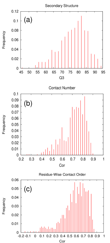
Figure 1: Histograms of accuracy measure obtained by ensemble predictions using 10 critical random networks. (a) $Q_{3}$ for secondary structure prediction; (b) $Cor$ for contact number prediction; (c) $Cor$ for residue-wise contact order prediction.

Secondary structure prediction

The average accuracy of secondary structure prediction achieved by the ensemble CRNs-based approach is $Q_{3}=77.8$% and $SOV=77.3$ (Table 1). This is comparable to the current state-of-the-art predictors such as PSIPRED[23]. The results in terms of per-residue accuracies ($Q_{s}$ and $Q_{s}^{pre}$) are listed in Table 2. The values of $Q_{s}$ suggest that the present method underestimates $\alpha$ helices ($H$) and, especially, $\beta$ strands ($E$) compared to coils $C$. However, when a residue is predicted as being $H$ or $E$, the probability of the correct prediction is rather high, especially for $E$ ($Q_{E}^{pre}=$ 79.9%). The histogram of $Q_{3}$ (Figure 1a) shows that the peak of the histogram resides well beyond $Q_{3}$ = 80%, and that only 20% of the predictions exhibit $Q_{3}$ of less than 70%. These observations demonstrate the capability of the CRNs-based prediction schemes.

Table 2: Summary of per-residue accuracies for SS predictions.

measure	$H$	$E$	$C$
$Q_{s}$	78.4	61.9	84.6
$Q_{s}^{pre}$	81.9	79.9	74.3
$MC$	0.704	0.636	0.602

Contact number prediction

Using an ensemble of CRNs, a correlation coefficient ($Cor$) of 0.726 and normalized RMS error ($DevA$) of 0.707 was achieved for CN predictions on average (Table 1). This result is a significant improvement over the previous method[4] which yielded $Cor=0.627$ and $DevA=0.941$. The median of the distribution of $Cor$ (Figure 1b) is 0.744, indicating that the majority of the predictions are of very high accuracy.

We have also examined the dependence of prediction accuracy on the structural class of target proteins (Table 3). Among all the structural classes, $\alpha/\beta$ proteins are predicted most accurately with $Cor=$ 0.757 and $DevA=$ 0.668. The accuracy for other classes do not differ qualitatively although all-$\beta$ proteins are predicted slightly less accurately.

Table 3: Summary of CN predictions for each SCOP class^a.

rangeb	SCOP classc
($Cor$)	a	b	c	d	e
(-1,0.5]	8	6	3	14	1
(0.5,0.6]	19	25	8	19	1
(0.6,0.7]	29	29	22	54	3
(0.7,0.8]	62	66	76	85	10
(0.8,0.9]	43	38	57	67	3
(0.9,1.0]	1	0	0	1	0
total	162	164	166	240	18
average $Cor$	0.721	0.712	0.757	0.728	0.722
average $DevA$	0.715	0.726	0.668	0.717	0.705

^a The number of occurrences of $Cor$ for the proteins in the test sets, classified according to the SCOP database; average values of $Cor$ and $DevA$ are also listed for each class.
^b The range “$(x,y]$” denotes $x<Cor\leq y$.
^c a: all-$\alpha$; b: all-$\beta$; c: $\alpha/\beta$; d: $\alpha+\beta$; e: multi-domain.

Residue-wise contact order prediction

For RWCO prediction, the average accuracy was such that $Cor$ = 0.601 and $DevA$ = 0.881. Although these figures appear to be poor compared to those of the CN prediction described above, they are yet statistically significant. The distribution of $Cor$ appears to be rather dispersed (Figure 1c), indicating that the prediction accuracy strongly depends on the characteristics of each target protein. In a similar manner as for CN, we also examined the dependence of prediction accuracy on the structural class of target proteins (Table 4). In this case, we have found a notable dependence of prediction accuracy on structural classes. The best accuracy is obtained for $\alpha+\beta$ proteins with $Cor=$ 0.629 and $DevA=$ 0.832. For these proteins, the distribution of $Cor$ also shows good tendency in that the fraction of poor predictions is relatively small (e.g., 14% for $Cor<$ 0.5). Interestingly, all-$\beta$ proteins also show good accuracies but all-$\alpha$ proteins are particularly poorly predicted. These observations suggest that the correlation between amino acid sequence and RWCO is strongly dependent on the structural class of the target protein. However, the rather dispersed distribution of $Cor$ for each class (Table 4) also suggests that there are more detailed effects of the global context on the accuracy of RWCO prediction.

Table 4: Summary of RWCO predictions for each SCOP class^a

range	SCOP class
($Cor$)	a	b	c	d	e
(-1,0.5]	58	31	46	34	6
(0.5,0.6]	29	37	31	56	4
(0.6,0.7]	41	27	33	65	5
(0.7,0.8]	24	47	40	72	3
(0.8,0.9]	10	22	16	13	0
total	162	164	166	240	18
average $Cor$	0.549	0.620	0.595	0.629	0.564
average $DevA$	0.981	0.869	0.857	0.832	0.957

^aSee Table 3 for notations.

Purely linear predictions with PSSMs

Almost all the modern methods for 1D structure prediction make use of PSSMs in combination with some kind of machine-learning techniques such as feed-forward or recurrent neural networks or support vector machines. The present study is no exception. Curiously, machine-learning approaches have become so widespread that no attempt appears to have been made to test simplest linear predictors based on PSSMs. In this subsection, we present results of 1D predictions using only the linear terms (Eq. 4) but without CRNs. In this prediction scheme, input is a local segment of a PSSM generated by PSI-BLAST, and a feature variable is predicted by a straight forward linear regression.

As can be clearly seen in Table 5, the results of the linear predictions are surprisingly good although not as good as with CRNs. For example, in SS prediction, the purely linear scheme achieved $Q_{3}$ = 75.2% which is lower than that of the CRNs-based scheme by only 3.6%. Although this is of course a large difference in a statistical sense, there may not be a discernible difference when individual predictions are concerned. (However, the improvement in the $SOV$ measure by using CRNs is quite large, indicating that the nonlinear terms in CRNs are indeed able to extract cooperative features.) It is widely accepted that the upper limit of accuracy ($Q_{3}$) of SS prediction based on a local window of a single sequence is less than 70%[25]. Therefore, more than 5% of the increase in $Q_{3}$ is brought simply by the use of PSSMs.

Similar observations also hold for CN and RWCO predictions (Table 5). In case of CN prediction, we have previously obtained $Cor$ = 0.555 by a simple linear method with single sequences[4]. Therefore, the effect of PSSMs is even more dramatic than SS prediction. This may be due to the fact that the most conspicuous feature of amino acid sequences conserved among distant homologs (as detected by PSI-BLAST) is the hydrophobicity of amino acid residues[26], which is closely related to contact numbers. Of course, the improvement by the use of PSSMs is largely made possible by the recent increase of amino acid sequence databases[27].

Table 5: Summary of prediction accuracies using only linear terms.

Struct.	Accuracy
SS	$Q_{3}$ = 75.2; $SOV$ = 72.7
CN	$Cor$ = 0.701; $DevA$ = 0.735
RWCO	$Cor$ = 0.584; $DevA$ = 0.902

The significance of criticality

The condition of criticality ($\beta=0.5$ in Eq. 10) is expected to enhance the extraction of the long-range correlations of an amino acid sequence, thus improving the prediction accuracy. To confirm this point, we tested the method by setting $\beta=0.1$ so that the network of state vectors is not at the critical point any more (otherwise the prediction and validation schemes were the same as above). The prediction accuracies obtained by these non-critical random networks were $Q_{3}=76.7$% and $SOV=76.6$ for SS, $Cor=0.716$ and $DevA=0.719$ for CN, and $Cor=0.589$ and $DevA=0.897$ for RWCO. These values are inferior to those obtained by the critical random networks (Table 1), although slightly better than the purely linear predictions (Table 5). Therefore, compared to the non-critical random networks, the critical random networks can indeed extract more information from amino acid sequence and improve the prediction accuracies.

Discussion

Comparison with other methods

Regarding the framework of 1D structure prediction, the critical random networks are most closely related to bidirectional recurrent neural networks (BRNNs)[28], in that both can treat a whole amino acid sequence rather than only a local window segment. The main differences are the following. First, network weights between input and hidden layers as well as those between hidden units are trained in BRNNs, whereas the corresponding weights in CRNs (random matrices $V$ and $W$, respectively, in Eq. 10) are fixed. Second, the output layer is nonlinear in BRNNs but linear in CRNs. Third, the network components that propagate sequence information from N-terminus to C-terminus are decoupled from those in the opposite direction in BRNNs, but they are coupled in CRNs.

Regarding the accuracy of SS prediction, BRNNs[29] and CRNs exhibit comparable results of $Q_{3}\approx$ 78%. However, a standard local window-based approach using feed-forward neural networks can also achieve this level of accuracy[23]. Thus, the CRNs-based method is not a single best predictor, but may serve as an addition to consensus predictions.

Although BRNNs have been also applied to CN prediction[30], contact numbers are predicted as 2-state categorical data (buried or exposed) so that the results cannot be directly compared. Nevertheless, we can convert CRNs-based real-value predictions into 2-state predictions. By using the same thresholds for the 2-state discretization as Pollastri et al.[30] (i.e., the average CN for each residue type), we obtained $Q_{2}=$ 75.6% per chain (75.1% per residue), and Matthews’ correlation coefficient $MC=$ 0.503 whereas those obtained by BRNNs are $Q_{2}=$ 73.9% (per residue) and $MC=$ 0.478. Therefore, for 2-state CN prediction, the present method yields more accurate results.

Since the present study is the very first attempt to predict RWCOs, there are no alternative methods to compare with. However, the comparison of CRNs-based methods for SS and CN predictions with other methods suggests that the accuracy of the RWCO prediction presented here may be the best possible result using any of the statistical learning methods currently available for 1D structure predictions.

Possibilities for further improvements

In the present study, we employed the simplest possible architecture for CRNs in which different sites are connected via nearest-neighbor interactions. A number of possibilities exist for the elaboration of the architecture. For example, we may introduce short-cuts between distant sites to treat non-local interactions more directly. Since the prediction accuracies depend on the structural context of target proteins (Tables 3 and 4), it may be also useful to include more global features of amino acid sequences such as the bias of amino acid composition or the average of PSSM components. These possibilities are to be pursued in future studies.

Conclusion

We have developed a novel method, CRNs-based regression, for predicting 1D protein structures from amino acid sequence. When combined with position-specific scoring matrices produced by PSI-BLAST, this method yields SS predictions as accurate as the best current predictors, CN predictions far better than previous methods, and RWCO predictions significantly correlated with observed values. We also examined the effect of PSSMs on prediction accuracy, and showed that most improvement is brought by the use of PSSMs although the further improvement due to the CRNs-based method is also significant. In order to achieve a qualitatively yet better predictions, however, it seems necessary to take into account other, more global, information than is provided by PSSMs.

References

- [1] Bonneau, R. and Baker, D. Ab initio protein structure prediction: progress and prospects. Annu. Rev. Biophys. Biomol. Struct. 30, 173–189, 2001.
- [2] Rost, B. Prediction in 1D: secondary structure, membrane helices, and accessibility. In Structural Bioinformatics, Bourne, P. E. and Weissig, H., editors, chapter 28, 559–587. Wiley-Liss, Inc., Hoboken, U.S.A., 2003.
- [3] Lee, B. and Richards, F. M. The interpretation of protein structures: Estimation of static accessibility. J. Mol. Biol. 55, 379–400, 1971.
- [4] Kinjo, A. R., Horimoto, K., and Nishikawa, K. Predicting absolute contact numbers of native protein structure from amino acid sequence. Proteins 58, 158–165, 2005.
- [5] Kinjo, A. R. and Nishikawa, K. Recoverable one-dimensional encoding of protein three-dimensional structures. Bioinformatics 21, 2167–2170, 2005. doi:10.1093/bioinformatics/bti330.
- [6] Nishikawa, K. and Ooi, T. Prediction of the surface-interior diagram of globular proteins by an empirical method. Int. J. Peptide Protein Res. 16, 19–32, 1980.
- [7] Sander, C. and Schneider, R. Database of homology-derived protein structures. Proteins 9, 56–68, 1991.
- [8] Jaeger, H. The “echo state” approach to analysing and training recurrent neural networks. Technical Report 148, GMD - German National Research Institute for Computer Science, , 2001.
- [9] Jaeger, H. and Haas, H. Harnessing nonlinearity: predicting chaotic systems and saving energy in wireless communication. Science 304, 78–80, 2004.
- [10] Altschul, S. F., Madden, T. L., Schaffer, A. A., Zhang, J., Zhang, Z., Miller, W., and Lipman, D. L. Gapped blast and PSI-blast: A new generation of protein database search programs. Nucleic Acids Res. 25, 3389–3402, 1997.
- [11] Kabsch, W. and Sander, C. Dictionary of protein secondary structure: Pattern recognition of hydrogen bonded and geometrical features. Biopolymers 22, 2577–2637, 1983.
- [12] Takahashi, W. Nonlinear functional analysis: Fixed point theorems and related topics. Kindai Kagaku Sha, Tokyo, , 1988. In Japanese.
- [13] Goldenfeld, N. Lectures on phase transitions and the renormalization group, volume 85 of Frontiers in physics. Addison-Wesley, Reading, Massachusetts, , 1992.
- [14] Haykin, S. Neural networks: A comprehensive foundation. Prentice-Hall, Upper Saddle River, New Jersey, 2nd edition, , 1999.
- [15] Kinjo, A. R. and Nishikawa, K. Predicting residue-wise contact orders of native protein structure from amino acid sequence. arXiv.org:q-bio.BM/0501015, , 2005.
- [16] Matsumoto, M. and Nishimura, T. Mersenne twister: a 623-dimensionally equidistributed uniform pseudorandom number generator. ACM Trans. Model. Comput. Simul. 8, 3–30, 1998.
- [17] Chandonia, J. M., Hon, G., Walker, N. S., Lo Conte, L., Koehl, P., Levitt, M., and Brenner, S. E. The astral compendium in 2004. Nucleic Acids Res. 32, D189–D192, 2004.
- [18] Murzin, A. G., Brenner, S. E., Hubbard, T., and Chothia, C. SCOP: A structural classification of proteins database for the investigation of sequences and structures. J. Mol. Biol. 247, 536–540, 1995.
- [19] Petersen, T. N., Lundegaard, C., Nielsen, M., Bohr, H., Bohr, J., Brunak, S., Gippert, G. P., and Lund, O. Prediction of protein secondary structure at 80% accuracy. Proteins 41, 17–20, 2000.
- [20] Tomii, K. and Akiyama, Y. FORTE: a profile-profile comparison tool for protein fold recognition. Bioinformatics 20, 594–595, 2004.
- [21] Tateno, Y., Saitou, N., Okubo, K., Sugawara, H., and Gojobori, T. DDBJ in collaboration with mass-sequencing teams on annotation. Nucleic Acids Res. 33, D25–D28, 2005.
- [22] Li, W., Jaroszewski, L., and Godzik, A. Tolerating some redundancy significantly speeds up clustering of large protein databases. Bioinformatics 18, 77–82, 2002.
- [23] Jones, D. T. Protein secondary structure prediction based on position-specific scoring matrices. J. Mol. Biol. 292, 195–202, 1999.
- [24] Zemla, A., Venclovas, C., Fidelis, K., and Rost, B. A modified definition of sov, a segment-based measure for protein secondary structure prediction assessment. Proteins 34, 220–223, 1999.
- [25] Crooks, G. E. and Brenner, S. E. Protein secondary structure: entropy, correlations and prediction. Bioinformatics 20, 1603–1611, 2004.
- [26] Kinjo, A. R. and Nishikawa, K. Eigenvalue analysis of amino acid substitution matrices reveals a sharp transition of the mode of sequence conservation in proteins. Bioinformatics 20, 2504–2508, 2004.
- [27] Przybylski, D. and Rost, B. Alignments grow, secondary structure prediction improves. Proteins 46, 197–205, 2002.
- [28] Baldi, P., Brunak, S., Frasconi, P., Soda, G., and Pollastri, G. Exploiting the past and the future in protein secondary structure prediction. Bioinformatics 15, 937–946, 1999.
- [29] Pollastri, G., Przybylski, D., Rost, B., and Baldi, P. Improving the prediction of protein secondary structure in three and eight classes using recurrent neural networks and profiles. Proteins 47, 228–235, 2002.
- [30] Pollastri, G., Baldi, P., Fariselli, P., and Casadio, R. Prediction of coordination number and relative solvent accessibility in proteins. Proteins 47, 142–153, 2002.