Variable selection from random forests: application to gene expression data

Abstract

Random forest is a classification algorithm well suited for microarray data: it shows excellent performance even when most predictive variables are noise, can be used when the number of variables is much larger than the number of observations, and returns measures of variable importance. Thus, it is important to understand the performance of random forest with microarray data and its use for gene selection.

We first show the effects of changes in parameters of random forest on the prediction error. Then we present an approach for gene selection that uses measures of variable importance and error rate, and is targeted towards the selection of small sets of genes. Using simulated and real microarray data, we show that the gene selection procedure yields small sets of genes while preserving predictive accuracy.

We first show the effects of changes in parameters of random forest on the prediction error rate with microarray data. Then we present two approaches for gene selection with random forest: 1) comparing variable importance plots of variable importance from original and permuted data sets; 2) using backwards variable elimination. Using simulated and real microarray data, we show: 1) variable importance plots can be used to recover the full set of genes related to the outcome of interest, without being adversely affected by collinearities; 2) backwards variable elimination yields small sets of genes while preserving predictive accuracy (compared to several state-of-the art algorithms). Thus, both methods are useful for gene selection.

All code is available as an R package, varSelRF, from CRAN http://cran.r-project.org/src/contrib/PACKAGES.html or from the supplementary material page.

Supplementary information: http://ligarto.org/rdiaz/Papers/rfVS/randomForestVarSel.html

1 Introduction

Random forest is an algorithm for classification developed by Leo Breiman (Breiman, 2001b, ) that uses an ensemble of classification trees (Breiman et al.,, 1984; Ripley,, 1996; Hastie et al.,, 2001). Each of the classification trees is built using a bootstrap sample of the data, and at each split the candidate set of variables is a random subset of the variables. Thus, random forest uses both bagging (bootstrap aggregation), a successful approach for combining unstable learners (Breiman,, 1996; Hastie et al.,, 2001), and random variable selection for tree building. Each tree is unpruned (grown fully), so as to obtain low-bias trees; at the same time, bagging and random variable selection result in low correlation of the individual trees. The algorithm yields an ensemble that can achieve both low bias and low variance (from averaging over a large ensemble of low-bias, high-variance but low correlation trees).

Random forest has excellent performance in classification tasks, comparable to support vector machines. Although random forest is not widely used in the microarray literature (but see Alvarez et al.,, 2005; Izmirlian,, 2004; Wu et al.,, 2003; Gunther et al.,, 2003; Man et al.,, 2004; Schwender et al.,, 2004), it has several characteristics that make it ideal for these data sets: a) can be used when there are many more variables than observations; b) has good predictive performance even when most predictive variables are noise; c) does not overfit; d) can handle a mixture of categorical and continuous predictors; e) incorporates interactions among predictor variables; f) the output is invariant to monotone transformations of the predictors; g) there are high quality and free implementations: the original Fortran code from L. Breiman and A. Cutler, and an R package from A. Liaw and M. Wiener (Liaw & Wiener,, 2002); h) there is little need to fine-tune parameters to achieve excellent performance; i) returns measures of variable (gene) importance. The most important parameter to choose is $mtry$, the number of input variables tried at each split, but it has been reported that the default value is often a good choice (Liaw & Wiener,, 2002). In addition, the user needs to decide how many trees to grow for each forest ($ntree$) as well as the minimum size of the terminal nodes ($nodesize$). These three parameters will be throughly examined in this paper.

Given these promising features, it is important to understand the performance of random forest compared to alternative state-of-the-art prediction methods with microarray data, as well as the effects of changes in the parameters of random forest. In this paper we present, as necessary background for the main topic of the paper (gene selection), the first through examination of these issues, including evaluating the effects of $mtry$, $ntree$ and $nodesize$ on error rate using nine real microarray data sets and simulated data.

The main question addressed in this paper is gene selection using random forest. A few authors have previously used variable selection with random forest. Dudoit & Fridlyand, (2003) and Wu et al., (2003) use filtering approaches and, thus, do not take advantage of the measures of variable importance returned by random forest as part of the algorithm. Svetnik et al., (2004) propose a method that is somewhat similar to our approach. The main difference is that Svetnik et al., (2004) first find the “best” dimension ($p$) of the model, and then choose the $p$ most important variables. This is a sound strategy when the objective is to build accurate predictors, without any regards for model interpretability. But this might not be the most appropriate for our purposes as it shifts the emphasis away from selection of specific genes, and in genomic studies the identity of the selected genes is relevant (e.g., to understand molecular pathways or to find targets for drug development).

The last issue addressed in this paper is the multiplicity (or lack of uniqueness or lack of stability) problem. Variable selection with microarray data can lead to many solutions that are equally good from the point of view of prediction rates, but that share few common genes. This multiplicity problem has been emphasized by Somorjai et al., (2003) and recent examples are shown in Ein-Dor et al., (2005) and Michielis et al., (2005). Although multiplicity of results is not a problem when the only objective of our method is prediction, it casts serious doubts on the biological interpretability of the results (Somorjai et al.,, 2003). Unfortunately most “methods papers” in bioinformatics do not evaluate the stability of the results obtained, leading to a false sense of trust on the biological interpretability of the output obtained. Our paper presents a through and critical evaluation of the stability of the lists of selected genes with the proposed (and two competing) methods.

2 Variable selection methods

2.1 Two objectives of variable selection

When facing gene selection problems, biomedical researchers often show interest in one of the following objectives:

1. To identify relevant genes for subsequent research; this involves obtaining a (probably large) set of genes that are related to the outcome of interest, and this set should include genes even if they perform similar functions and are highly correlated.

2. To identify small sets of genes to be used for diagnostic purposes in clinical practice; this involves obtaining the smallest possible set of genes that can still achieve good predictive performance (thus, “redundant” genes should not be selected).

We will focus on the second objective. The use of random forest for the first objective is under investigation and will be reported elsewhere.

2.2 Variable importance from random forest

Random forest returns several measures of variable importance. The most reliable measure is based on the decrease of classification accuracy when values of a variable in a node of a tree are permuted randomly (Breiman, 2001b, ; Bureau et al.,, 2003), and this is the measure of variable importance (in its unscaled version —see supplementary material) that we will use in the rest of the paper.

2.3 Backwards elimination of variables (genes) using OOB error

To select gebes we can iteratively fit random forests, at each iteration building a new forest after discarding those variables (genes) with the smallest variable importances; the selected set of genes is the one that yields the smallest error rate. Random forest returns a measure of error rate based on the out-of-bag cases for each fitted tree, the OOB error, and this is the measure of error we will use. Note that in this section we are using OOB error to choose the final set of genes, not to obtain unbiased estimates of the error rate of this rule. Because of the iterative approach, the OOB error is biased down and cannot be used to asses the overall error rate of the approach, for reasons analogous to those leading to “selection bias” (Ambroise & McLachlan,, 2002; Simon et al., 2003a, ). To assess prediction error rates we will use the bootstrap, not OOB error (see section 3.3). (Using error rates affected by selection bias to select the optimal number of genes is not necessarily a bad procedure from the point of view of selecting the final number of genes; see Braga-Neto et al., (2004)).

In our algorithm we examine all forests that result from eliminating, iteratively, a fraction, $fraction.dropped$, of the genes (the least important ones) used in the previous iteration. By default, $fraction.dropped=0.2$ which allows for relatively fast operation, is coherent with the idea of an “aggressive variable selection” approach, and increases the resolution as the number of genes considered becomes smaller. We do not recalculate variable importances at each step as Svetnik et al., (2004) mention severe overfitting resulting from recalculating variable importances. After fitting all forests, we examine the OOB error rates from all the fitted random forests. We choose the solution with the smallest number of genes whose error rate is within $u$ standard errors of the minimum error rate of all forests. Setting $u=0$ is the same as selecting the set of genes that leads to the smallest error rate. Setting $u=1$ is similar to the common “1 s.e. rule”, used in the classification trees literature (Ripley,, 1996; Breiman et al.,, 1984); this strategy can lead to solutions with fewer genes than selecting the solution with the smallest error rate, while achieving an error rate that is not different, within sampling error, from the “best solution”. In this paper we will examine both the “1 s.e. rule” and the “0 s.e. rule”.

3 Evaluation of performance

3.1 Data sets

We have used both simulated and real microarray data sets to evaluate the variable selection procedure. For the real data sets, original reference paper and main features are shown in Table 1. Further details are provided in the supplementary material.

Table 1: Main characteristics of the microarray data sets used.

Dataset	Original ref.	Genes	Patients	Classes
Leukemia	Golub et al., (1999)	3051	38	2
Breast	van ’t Veer et al., (2002)	4869	78	2
Breast	van ’t Veer et al., (2002)	4869	96	3
NCI 60	Ross et al., (2000)	5244	61	8
Adenocar-
cinoma	Ramaswamy et al., (2003)	9868	76	2
Brain	Pomeroy et al., (2002)	5597	42	5
Colon	Alon et al., (1999)	2000	62	2
Lymphoma	Alizadeh et al., (2000)	4026	62	3
Prostate	Singh et al., (2002)	6033	102	2
Srbct	Khan et al., (2001)	2308	63	4

To evaluate if the proposed procedure can recover the signal in the data, we need to use simulated data, so that we know exactly which genes are relevant. Data have been simulated using different numbers of classes of patients (2 to 4), number of independent dimensions (1 to 3), and number of genes per dimension (5, 20, 100). In all cases, we have set to 25 the number of subjects per class. Each independent dimension has the same relevance for discrimination of the classes. The data come from a multivariate normal distribution with variance of 1, a (within-class) correlation among genes within dimension of 0.9, and a within-class correlation of 0 between genes from different dimensions, as those are independent. The multivariate means have been set so that the unconditional prediction error rate (McLachlan,, 1992) of a linear discriminant analysis using one gene from each dimension is approximately 5%. To each data set we have added 2000 random normal variates (mean 0, variance 1) and 2000 random uniform $[-1,1]$ variates. In addition, we have generated data sets for 2, 3, and 4 classes where no genes have signal (all 4000 genes are random). For the non-signal data sets we have generated four replicate data sets for each level of number of classes. Further details are provided in the supplementary material.

3.2 Competing methods

We have compared the predictive performance of the variable selection approach with: a) random forest without any variable selection (using $mtry=\sqrt{number\ of\ genes}$, $ntree=5000$, $nodesize=1$); b) three other methods that have shown good performance in reviews of classification methods with microarray data (Dudoit et al.,, 2002; Romualdi et al.,, 2003; Dettling,, 2004) but that do not include any variable selection; c) two methods that carry out variable selection.

For the three methods that do not carry out variable selection, Diagonal Linear Discriminant Analysis (DLDA), K nearest neighbor (KNN), and Support Vector Machines (SVM) with linear kernel, we have used, based on Dudoit et al., (2002), the 200 genes with the largest $F$-ratio of between to within groups sums of squares. For KNN, the number of neighbors ($K$) was chosen by cross-validation as in Dudoit et al., (2002).

One of the methods that incorporates gene selection is Shrunken centroids (SC), developed by Tibshirani et al., (2002). We have used two different approaches to determine the best number of features. In the first one, SC.l, we choose the number of genes that minimizes the cross-validated error rate and, in case of several solutions with minimal error rates, we choose the one with largest likelihood. In the second approach, SC.s, we choose the number of genes that minimizes the cross-validated error rate and, in case of several solutions with minimal error rates, we choose the one with smallest number of genes (larger penalty). The second method that incorporates gene selection is Nearest neighbor + variable selection (NN.vs), where we filter genes using the F-ratio, and select the number of genes that leads to the smallest error rate; in our implementation, we run a Nearest Neighbor classifier (KNN with K = 1) on all subsets of genes that result from eliminating $20\%$ of the genes (the ones with the smallest F-ratio) used in the previous iteration. This approach, in its many variants (changing both the classifier and the ordering criterion) is popular in microarray papers; a recent example is Roepman et al., (2005), and similar general strategies are implemented in the program Tnasas (Herrero et al.,, 2004). Further details of all these methods are provided in the supplementary material. All simulations and analyses were carried out with R (http://www.r-project.org; R Development Core Team,, 2004), using packages randomForest (from A. Liaw and M. Wiener) for random forest, e1071 (E. Dimitriadou, K. Hornik, F. Leisch, D. Meyer, and A. Weingessel) for SVM, class (B. Ripley and W. Venables) for KNN, PAM (Tibshirani et al.,, 2002) for shrunken centroids, and geSignatures (by R.D.-U.) for DLDA.

3.3 Estimation of error rates

To estimate the prediction error rate of all methods we have used the .632+ bootstrap method (Ambroise & McLachlan,, 2002; Efron & Tibshirani,, 1997). It must be emphasized that the error rate used when performing variable selection is not the error rate reported as the prediction error rate (e.g., Table 2), nor the error used to compute the .632+ estimate. To calculate the prediction error rate (as reported, for example, in Table 2) the .632+ bootstrap method is applied to the complete procedure, and thus the “out-of-bag” samples used in the .632+ method are samples that are not used when fitting the random forest, or carrying out variable selection. This also applies when evaluating the competing methods.

3.4 Stability (uniqueness) of results

Following Faraway, (1992), Harrell, (2001), and Efron & Gong, (1983), we have evaluated the stability of the variable selection procedure using the bootstrap. This allows us to asses how often a given gene, selected when running the variable selection procedure in the original sample, is selected when running the procedure on bootstrap samples.

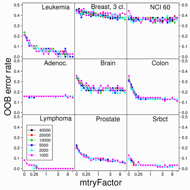
Figure 1: Out-of-Bag (OOB) vs $mtryFactor$ for the nine microarray data sets. $mtryFactor$ is the multiplicative factor of the default $mtry$ ($\sqrt{number.of.genes}$); thus, an $mtryFactor$ of 3 means the number of genes tried at each split is $3*\sqrt{number.of.genes}$; an $mtryFactor=0$ means the number of genes tried was 1; the $mtryFactor$s examined were $=\{0,0.05,0.1,0.17,0.25,0.33,0.5,0.75,0.8,1,1.15,1.33,1.5,2,3,$ $4,5,6,8,10,13\}$. Results shown for six different $ntree=\{1000,2000,5000,10000,20000,40000\}$. $nodesize=1$.

4 Results

Table 2: Error rates (estimated using the 0.632+ bootstrap method with 200 bootstrap samples) for the microarray data sets using different methods (see text for description of alternative methods). The results shown for variable selection with random forest used $ntree=2000,fraction.dropped=0.2,mtryFactor=1$. Note that the OOB error used for variable selection is not the error reported in this table; the error rate reported is obtained using bootstrap on the complete variable selection process. The column “no info” denotes the minimal error we can make if we use no information from the genes (i.e., we always bet on the most frequent class).

Data set	no info	SVM	KNN	DLDA	SC.l	SC.s	NN.vs	random forest	random forest var.sel.
									s.e. 0	s.e. 1
Leukemia	0.289	0.014	0.029	0.020	0.025	0.062	0.056	0.051	0.087	0.075
Breast 2 cl.	0.429	0.325	0.337	0.331	0.324	0.326	0.337	0.342	0.337	0.332
Breast 3 cl.	0.537	0.380	0.449	0.370	0.396	0.401	0.424	0.351	0.346	0.364
NCI 60	0.852	0.256	0.317	0.286	0.256	0.246	0.237	0.252	0.327	0.353
Adenocar.	0.158	0.203	0.174	0.194	0.177	0.179	0.181	0.125	0.185	0.207
Brain	0.761	0.138	0.174	0.183	0.163	0.159	0.194	0.154	0.216	0.216
Colon	0.355	0.147	0.152	0.137	0.123	0.122	0.158	0.127	0.159	0.177
Lymphoma	0.323	0.010	0.008	0.021	0.028	0.033	0.04	0.009	0.047	0.042
Prostate	0.490	0.064	0.100	0.149	0.088	0.089	0.081	0.077	0.061	0.064
Srbct	0.635	0.017	0.023	0.011	0.012	0.025	0.031	0.021	0.039	0.038

4.1 Choosing $mtry$ and $ntree$

Preliminary data suggested that $mtry$ and $ntree$ could affect the shape of variable importance plots. At the same time, use of OOB error rate as a guidance to select $mtry$ could be affected by $ntree$ and, potentially, $nodesize$. Thus, we first examined whether the OOB error rate is substantially affected by changes in $mtry$, $ntree$, and $nodesize$.

Figure 1 and the supplementary material (Figure
“error.vs.mtry.pdf”), however, show that, for both real and simulated data, the relation of OOB error rate with $mtry$ is largely independent of $ntree$ (for $ntree$ between 1000 and 40000) and $nodesize$ (nodesizes 1 and 5). In addition, the default setting of $mtry$ ($mtryFactor=1$ in the figures) is often a good choice in terms of OOB error rate. In some cases, increasing $mtry$ can lead to small decreases in error rate, and decreases in $mtry$ often lead to increases in the error rate. This is specially the case with simulated data with very few relevant genes (with very few relevant genes, small $mtry$ results in many trees being built that do not incorporate any of the relevant genes). Since the OOB error and the relation between OOB error and $mtry$ do not change whether we use $nodesize$ of 1 or 5, and because the increase in speed from using $nodesize$ of 5 is inconsequential, all further analyses will use only the default $nodesize=1$.

4.2 Backwards elimination of variables (genes) using OOB error

On the simulated data sets (see supplementary material, Tables 3 and 4) backwards elimination often leads to very small sets of genes, often much smaller than the set of “true genes”. The error rate of the variable selection procedure, estimated using the .632+ bootstrap method, indicates that the variable selection procedure does not lead to overfitting, and can achieve the objective of aggressively reducing the set of selected genes. In contrast, when the simplification procedure is applied to simulated data sets without signal (see Tables 1 and 2 in supplementary material), the number of genes selected is consistently much larger and, as should be the case, the estimated error rate using the bootstrap corresponds to that achieved by always betting on the most probable class.

Results for the real data sets are shown in Tables 2 and 3 (see also supplementary material, Tables 5, 6, 7, for additional results using different combinations of $ntree=\{2000,5000,20000\}$, $mtryFactor=\{1,13\},se=\{0,1\},fraction.dropped=\{0.2,0.5\}$). Error rates (see Table 2) when performing variable selection are in most cases comparable (within sampling error) to those from random forest without variable selection, and comparable also to the error rates from competing state-of-the-art prediction methods. The number of genes selected varies by data set, but generally (Table 3) the variable selection procedure leads to small ($<50$) sets of predictor genes, often much smaller than those from competing approaches (see also Table 8 in supplementary material). There are no relevant differences in error rate related to differences in $mtry$, $ntree$ or whether we use the “s.e. 1” or “s.e. 0” rules. The use of the “s.e. 1” rule, however, tends to result in smaller sets of selected genes.

4.3 Stability (uniqueness) of results

The results here will focus on the real microarray data sets (results from the simulated data are presented on the supplementary material). Table 3 (see also supplementary material, Tables 5, 6, 7, for other combinations of $ntree,mtryFactor,fraction.dropped,se$) shows the variation in the number of genes selected in bootstrap samples, and the frequency with which the genes selected in the original sample appear among the genes selected from the bootstrap samples. In most cases, there is a wide range in the number of genes selected; more importantly, the genes selected in the original samples are rarely selected in more than 50% of the bootstrap samples. These results are not strongly affected by variations in $ntree$ or $mtry$; using the “s.e. 1” rule can lead, in some cases, to increased stability of the results.

As a comparison, we also show in Table 3 the stability of two alternative approaches for gene selection, the shrunken centroids method, and a filter approach combined with a Nearest Neighbor classifier (see Table 8 in the supplementary material for results of SC.l). Error rates are comparable, but both alternative methods lead to much larger sets of selected genes than backwards variable selection with random forests. The alternative approaches seem to lead to somewhat more stable results in variable selection (probably a consequence of the large number of genes selected) but in practical applications this increase in stability is probably far out-weighted by the very large number of selected genes.

Table 3: Stability of variable (gene) selection evaluated using 200 bootstrap samples. “# Genes”: number of genes selected on the original data set. “# Genes boot.”: median (1st quartile, 3rd quartile) of number of genes selected from on the bootstrap samples. “Freq. genes”: median (1st quartile, 3rd quartile) of the frequency with which each gene in the original data set appears in the genes selected from the bootstrap samples. Parameters for backwards elimination with random forest: $mtryFactor=1,s.e.\ =0,ntree=2000,ntreeIterat=1000,fraction.dropped=0.2$.

Data set	Error	# Genes	# Genes boot.	Freq. genes
Backwards elimination of genes from random forest
$s.e.\ =0$
Leukemia	0.087	2	2 (2, 2)	0.38 (0.29, 0.48)
Breast 2 cl.	0.337	14	9 (5, 23)	0.15 (0.1, 0.28)
Breast 3 cl.	0.346	110	14 (9, 31)	0.08 (0.04, 0.13)
NCI 60	0.327	230	60 (30, 94)	0.1 (0.06, 0.19)
Adenocar.	0.185	6	3 (2, 8)	0.14 (0.12, 0.15)
Brain	0.216	22	14 (7, 22)	0.18 (0.09, 0.25)
Colon	0.159	14	5 (3, 12)	0.29 (0.19, 0.42)
Lymphoma	0.047	73	14 (4, 58)	0.26 (0.18, 0.38)
Prostate	0.061	18	5 (3, 14)	0.22 (0.17, 0.43)
Srbct	0.039	101	18 (11, 27)	0.1 (0.04, 0.29)
$s.e.\ =1$
Leukemia	0.075	2	2 (2, 2)	0.4 (0.32, 0.5)
Breast 2 cl.	0.332	14	4 (2, 7)	0.12 (0.07, 0.17)
Breast 3 cl.	0.364	6	7 (4, 14)	0.27 (0.22, 0.31)
NCI 60	0.353	24	30 (19, 60)	0.26 (0.17, 0.38)
Adenocar.	0.207	8	3 (2, 5)	0.06 (0.03, 0.12)
Brain	0.216	9	14 (7, 22)	0.26 (0.14, 0.46)
Colon	0.177	3	3 (2, 6)	0.36 (0.32, 0.36)
Lymphoma	0.042	58	12 (5, 73)	0.32 (0.24, 0.42)
Prostate	0.064	2	3 (2, 5)	0.9 (0.82, 0.99)
Srbct	0.038	22	18 (11, 34)	0.57 (0.4, 0.88)
Alternative approaches
SC.s
Leukemia	0.062	82	46 (14, 504)	0.48 (0.45, 0.59)
Breast 2 cl.	0.326	31	55 (24, 296)	0.54 (0.51, 0.66)
Breast 3 cl.	0.401	2166	4341 (2379, 4804)	0.84 (0.78, 0.88)
NCI 60	0.246	5118	4919 (3711, 5243)	0.84 (0.74, 0.92)
Adenocar.	0.179	0	9 (0, 18)	NA (NA, NA)
Brain	0.159	4177	1257 (295, 3483)	0.38 (0.3, 0.5)
Colon	0.122	15	22 (15, 34)	0.8 (0.66, 0.87)
Lymphoma	0.033	2796	2718 (2030, 3269)	0.82 (0.68, 0.86)
Prostate	0.089	4	3 (2, 4)	0.72 (0.49, 0.92)
Srbct	0.025	37	18 (12, 40)	0.45 (0.34, 0.61)
NN.vs
Leukemia	0.056	512	23 (4, 134)	0.17 (0.14, 0.24)
Breast 2 cl.	0.337	88	23 (4, 110)	0.24 (0.2, 0.31)
Breast 3 cl.	0.424	9	45 (6, 214)	0.66 (0.61, 0.72)
NCI 60	0.237	1718	880 (360, 1718)	0.44 (0.34, 0.57)
Adenocar.	0.181	9868	73 (8, 1324)	0.13 (0.1, 0.18)
Brain	0.194	1834	158 (52, 601)	0.16 (0.12, 0.25)
Colon	0.158	8	9 (4, 45)	0.57 (0.45, 0.72)
Lymphoma	0.04	15	15 (5, 39)	0.5 (0.4, 0.6)
Prostate	0.081	7	6 (3, 18)	0.46 (0.39, 0.78)
Srbct	0.031	11	17 (11, 33)	0.7 (0.66, 0.85)

^∗Only two genes are selected from the complete data set; the values are the actual frequencies of those two genes.
^†Tibshirani et al., (2002) select 21 genes after visually inspecting the plot of cross-validation error rate vs. amount of shrinkage and number of genes. Their procedure is hard to automate and thus it is very difficult to obtain estimates of the error rate of their procedure.
^‡Tibshirani et al., (2002) select 43 genes. The difference is likely due to differences in the random partitions for cross-validation. Repeating 100 times the gene selection process with the full data set the median, 1st quartile, and 3rd quartile of the number of selected genes are 13, 8, and 147.

5 Discussion

We have examined the performance of an approach for gene selection using random forest, and compared it to alternative approaches. Our results, using both simulated and real microarray data sets, show that this method of gene selection accomplishes the proposed objectives. Our method returns very small sets of genes compared to two alternative variable selection methods, while retaining predictive performance comparable to that of seven alternative state-of-the-art methods. Recently, Yeung et al., (2005) have proposed a Bayesian model averaging (BMA) approach for gene selection; comparing the results for the two common data sets between our study and theirs, in one case (Leukemia) our procedure returns a much smaller set of genes (2 vs. 15), whereas in another (Breast, 2 class) their BMA procedure returns 8 fewer genes (14 vs. 6); our procedure does not require setting a limit in the maximum number of relevant genes to be selected nor does it require to prespecify a number of top ranked genes as relevant (the latter is nor required by the BMA procedure either).

Our method of gene selection will not return sets of genes that are highly correlated, because they are redundant. This method will be most useful under two scenarios: a) when considering the design of diagnostic tools, where having a small set of probes is often desirable; b) to help understand the results from other gene selection approaches that return many genes, so as to understand which ones of those genes have the largest signal to noise ratio and could be used as surrogates for complex processes involving many correlated genes. A backwards elimination method, precursor to the one used here, has been already used to predict breast tumor type based on chromosomic alterations (Alvarez et al.,, 2005).

We have also throughly examined the effects of changes in the parameters of random forest (specifically $mtry$, $ntree$, $nodesize$) and the variable selection algorithm ($se$, $fraction.dropped$). Changes in these parameters have in most cases negligible effects, suggesting that the default values are often good options, but we can make some general recommendations. Time of execution of the code increases $\approx$ linearly with $ntree$. Larger $ntree$ values lead to slightly more stable values of variable importances, but for the data sets examined, $ntree=2000$ or $ntree=5000$ seem quite adequate, with further increases having negligible effects. The change in $nodesize$ from 1 to 5 has negligible effects, and thus its default setting of 1 is appropriate. For the backwards elimination algorithm, the parameter $fraction.dropped$ can be adjusted to modify the resolution of the number of variable selected; smaller values of $fraction.dropped$ lead to finer resolution in the examination of number of genes, but to slower execution of the code. Finally, the parameter $se$ has also minor effects on the results of the backwards variable selection algorithm but a value of $se=1$ leads to slightly more stable results.

The final issue addressed in this paper is instability or multiplicity of the selected sets of genes. From this point of view, the results are slightly disappointing. But so are the results of the competing methods. And so are the results of most examined methods so far with microarray data, as shown in Ein-Dor et al., (2005) and Michielis et al., (2005) and discussed throughly by Somorjai et al., (2003) for classification and by Pan et al., (2005) for the related problem of the effect of threshold choice in gene selection. However, and except for the above cited papers and the review in Díaz-Uriarte, (2005), this is an issue that still seems largely ignored in the microarray literature. As these papers and the statistical literature on variable selection (e.g., Breiman, 2001a, ; Harrell,, 2001) discusses, the causes of the problem are small sample sizes and the extremely small ratio of samples to variables (i.e., number of arrays to number of genes). Thus, we might need to learn to live with the problem, and try to assess the stability and robustness of our results by using a variety of gene selection features, and examining whether there is a subset of features that tends to be repeatedly selected. This concern is explicitly taken into account in our results, and facilities for examining this problem are part of our R code.

The multiplicity problem, however, does not need to result in large prediction errors. This and other papers (Dudoit et al.,, 2002; Dettling & Bühlmann,, 2004; Simon et al., 2003b, ; Romualdi et al.,, 2003; Dettling,, 2004; Somorjai et al.,, 2003) show that very different classifiers often lead to comparable and successful error rates with a variety of microarray data sets. Thus, although improving prediction rates is important (specially if giving consideration to ROC curves, and not just overall prediction error rates; Pepe,, 2003), when trying to address questions of biological mechanism or discover therapeutic targets, probably a more challenging and relevant issue is to identify sets of genes with biological relevance.

Two areas of future research are using random forest for the selection of potentially large sets of genes that include correlated genes, and improving the computational efficiency of these approaches; in the present work, we have used parallelization of the “embarrassingly parallelizable” tasks using MPI with the Rmpi and Snow packages (Yu,, 2004; Tierney et al.,, 2004) for R. In a broader context, further work is warranted on the stability properties and biological relevance of this and other gene-selection approaches, because the multiplicity problem casts doubts on the biological interpretability of most results based on a single run of one gene-selection approach.

6 Conclusion

The proposed method can be used for variable selection fulfilling the objectives above: we can obtain very small sets of non-redundant genes while preserving predictive accuracy. These results clearly indicate that the proposed method can be profitably used with microarray data. Given its performance, random forest and variable selection using random forest should probably become part of the “standard tool-box” of methods for the analysis of microarray data.

7 Acknowledgements

Most of the simulations and analyses were carried out in the Beowulf cluster of the Bioinformatics unit at CNIO, financed by the RTICCC from the FIS; J. M. Vaquerizas provided help with the administration of the cluster. A. Liaw provided discussion, unpublished manuscripts, and code. C. Lázaro-Perea provided many discussions and comments on the ms. A. Sánchez provided comments on the ms. I. Díaz showed R.D.-U. the forest, or the trees, or both. R.D.-U. partially supported by the Ramón y Cajal program of the Spanish MEC (Ministry of Education and Science); S.A.A. supported by project C.A.M. GR/SAL/0219/2004; funding provided by project TIC2003-09331-C02-02 of the Spanish MEC.

References

- Alizadeh et al., (2000) Alizadeh, A. A., Eisen, M. B., Davis, R. E., Ma, C., Lossos, I. S., Rosenwald, A., Boldrick, J. C., Sabet, H., Tran, T., Yu, X., Powell, J. I., Yang, L., Marti, G. E., Moore, T., Hudson Jr, J., Lu, L., Lewis, D. B., Tibshirani, R., Sherlock, G., Chan, W. C., Greiner, T. C., Weisenburger, D. D., Armitage, J. O., Warnke, R., Levy, R., Wilson, W., Grever, M. R., Byrd, J. C., Botstein, D., Brown, P. O. & Staudt, L. M. (2000) Distinct types of diffuse large B-cell lymphoma identified by gene expression profiling. Nature, 403, 503–511.
- Alon et al., (1999) Alon, U., Barkai, N., Notterman, D. A., Gish, K., Ybarra, S., Mack, D. & Levine, A. J. (1999) Broad patterns of gene expression revealed by clustering analysis of tumor and normal colon tissues probed by oligonucleotide arrays. Proc Natl Acad Sci U S A, 96, 6745–6750.
- Alvarez et al., (2005) Alvarez, S., Diaz-Uriarte, R., Osorio, A., Barroso, A., Melchor, L., Paz, M. F., Honrado, E., Rodriguez, R., Urioste, M., Valle, L., Diez, O., Cigudosa, J. C., Dopazo, J., Esteller, M. & Benitez, J. (2005) A Predictor Based on the Somatic Genomic Changes of the BRCA1/BRCA2 Breast Cancer Tumors Identifies the Non-BRCA1/BRCA2 Tumors with BRCA1 Promoter Hypermethylation. Clin Cancer Res, 11, 1146–1153.
- Ambroise & McLachlan, (2002) Ambroise, C. & McLachlan, G. J. (2002) Selection bias in gene extraction on the basis of microarray gene-expression data. Proc Natl Acad Sci USA, 99 (10), 6562–6566.
- Braga-Neto et al., (2004) Braga-Neto, U., Hashimoto, R., Dougherty, E. R., Nguyen, D. V. & Carroll, R. J. (2004) Is cross-validation better than resubstitution for ranking genes? Bioinformatics, 20, 253–258.
- Breiman, (1996) Breiman, L. (1996) Bagging predictors. Machine Learning, 24, 123–140.
- (7) Breiman, L. (2001a) Statistical modeling: the two cultures (with discussion). Statistical Science, 16, 199–231.
- (8) Breiman, L. (2001b) Random forests. Machine Learning, 45, 5–32.
- Breiman et al., (1984) Breiman, L., Friedman, J., Olshen, R. & Stone, C. (1984) Classification and regression trees. Chapman & Hall, New York.
- Bureau et al., (2003) Bureau, A., Dupuis, J., Hayward, B., Falls, K. & Van Eerdewegh, P. (2003) Mapping complex traits using Random Forests. BMC Genet, 4 Suppl 1, S64.
- Dettling, (2004) Dettling, M. (2004) Bagboosting for tumor classification with gene expression data. Bioinformatics, 20, 3583–593.
- Dettling & Bühlmann, (2004) Dettling, M. & Bühlmann, P. (2004) Finding predictive gene groups from microarray data. J. Multivariate Anal., 90, 106–131.
- Díaz-Uriarte, (2005) Díaz-Uriarte, R. (2005) Supervised methods with genomic data: a review and cautionary view. In F. Azuaje and J. Dopazo (eds.) Data analysis and visualization in genomics and proteomics. New York: Wiley pp. 193–214.
- Dudoit & Fridlyand, (2003) Dudoit, S. & Fridlyand, J. (2003) Classification in microarray experiments. In T. Speed (ed.) Statistical analysis of gene expression microarray data. New York: Chapman & Hall pp. 93–158.
- Dudoit et al., (2002) Dudoit, S., Fridlyand, J. & Speed, T. P. (2002) Comparison of discrimination methods for the classification of tumors suing gene expression data. J Am Stat Assoc, 97 (457), 77–87.
- Efron & Gong, (1983) Efron, B. & Gong, G. (1983) A leisurely look at the bootstrap, the jacknife, and cross-validation. The American Statistician, 37, 36–48.
- Efron & Tibshirani, (1997) Efron, B. & Tibshirani, R. J. (1997) Improvements on cross-validation: the .632+ bootstrap method. J. American Statistical Association, 92, 548–560.
- Ein-Dor et al., (2005) Ein-Dor, L., Kela, I., Getz, G., Givol, D. & Domany, E. (2005) Outcome signature genes in breat cancer: is there a unique set? Bioinformatics, 21, 171–178.
- Faraway, (1992) Faraway, J. (1992) On the cost of data analysis. Journal of Computational and Graphical Statistics, 1, 251–231.
- Friedman & Meulman, (2005) Friedman, J. & Meulman, J. (2005) Clustering objects on subsets of attributes (with discussion). J. Royal Statistical Society, Series B, 66, 815–850.
- Golub et al., (1999) Golub, T. R., Slonim, D. K., Tamayo, P., Huard, C., Gaasenbeek, M., Mesirov, J. P., Coller, H., Loh, M. L., Downing, J. R., Caligiuri, M. A., Bloomfield, C. D. & Lander, E. S. (1999) Molecular classification of cancer: class discovery and class prediction by gene expression monitoring. Science, 286, 531–537.
- Gunther et al., (2003) Gunther, E. C., Stone, D. J., Gerwien, R. W., Bento, P. & Heyes, M. P. (2003) Prediction of clinical drug efficacy by classification of drug-induced genomic expression profiles in vitro. Proc Natl Acad Sci U S A, 100, 9608–9613.
- Harrell, (2001) Harrell, J. F. E. (2001) Regression modeling strategies. Springer, New York.
- Hastie et al., (2001) Hastie, T., Tibshirani, R. & Friedman, J. (2001) The elements of statistical learning. Springer, New York.
- Herrero et al., (2004) Herrero, J., Vaquerizas, J.M., Al-Shahrour, F., Conde, L., Mateos, Á., Santoyo, J., Díaz-Uriarte, R. & Dopazo, J. (2004). New challenges in gene expression data analysis and the extended GEPAS. Nucleic Acids Research 32 (Web Server issue), W485–W491.
- Izmirlian, (2004) Izmirlian, G. (2004) Application of the random forest classification algorithm to a SELDI-TOF proteomics study in the setting of a cancer prevention trial. Ann N Y Acad Sci, 1020, 154–174.
- Jolliffe, (2002) Jolliffe, I. T. (2002) Principal component analysis, 2nd ed. Springer, New York.
- Khan et al., (2001) Khan, J., Wei, J. S., Ringner, M., Saal, L. H., Ladanyi, M., Westermann, F., Berthold, F., Schwab, M., Antonescu, C. R., Peterson, C. & Meltzer, P. S. (2001) Classification and diagnostic prediction of cancers using gene expression profiling and artificial neural networks. Nat Med, 7, 673–679.
- Liaw & Wiener, (2002) Liaw, A. & Wiener, M. (2002) Classification and regression by randomforest. Rnews, 2, 18–22.
- Man et al., (2004) Man, M. Z., Dyson, G., Johnson, K. & Liao, B. (2004) Evaluating methods for classifying expression data. J Biopharm Statist, 14, 1065–1084.
- McLachlan, (1992) McLachlan, G. J. (1992) Discriminant analysis and statistical pattern recognition. Wiley, New York.
- Michielis et al., (2005) Michielis, S., Koscielny, S. & Hill, C. (2005). Prediction of cnacer outcome with microarrays: a multiple random validation strategy. The Lancet, 365, 488–492.
- Pan et al., (2005) Pan, K.-H., Lih, C.-J., & Cohen, S. N. (2005) Effects of threshold choice on the biological conclusions reached during the analysis of gene expression by DNA microarrays. PNAS,102, 8961–8965.
- Pepe, (2003) Pepe, M. S. (2003) The statistical evaluation of medical tests for classification and prediction. Oxford Univeristy Press, Oxford.
- Pomeroy et al., (2002) Pomeroy, S. L., Tamayo, P., Gaasenbeek, M., Sturla, L. M., Angelo, M., McLaughlin, M. E., Kim, J. Y., Goumnerova, L. C., Black, P. M., Lau, C., Allen, J. C., Zagzag, D., Olson, J. M., Curran, T., Wetmore, C., Biegel, J. A., Poggio, T., Mukherjee, S., Rifkin, R., Califano, A., Stolovitzky, G., Louis, D. N., Mesirov, J. P., Lander, E. S. & Golub, T. R. (2002) Prediction of central nervous system embryonal tumour outcome based on gene expression. Nature, 415, 436–442.
- R Development Core Team, (2004) R Development Core Team (2004) R: A language and environment for statistical computing. R Foundation for Statistical Computing Vienna, Austria. 3-900051-07-0.
- Ramaswamy et al., (2003) Ramaswamy, S., Ross, K. N., Lander, E. S. & Golub, T. R. (2003) A molecular signature of metastasis in primary solid tumors. Nature Genetics, 33, 49–54.
- Ripley, (1996) Ripley, B. D. (1996) Pattern recognition and neural networks. Cambridge University Press, Cambridge.
- Roepman et al., (2005) Roepman, P., Wessels, L. F., Kettelarij, N., Kemmeren, P., Miles, A. J., Lijnzaad, P., Tilanus, M. G., Koole, R., Hordijk, G. J., van der Vliet, P. C., Reinders, M. J., Slootweg, P. J. & Holstege, F. C. (2005) An expression profile for diagnosis of lymph node metastases from primary head and neck squamous cell carcinomas. Nat Genet, 37, 182–186.
- Romualdi et al., (2003) Romualdi, C., Campanaro, S., Campagna, D., Celegato, B., Cannata, N., Toppo, S., Valle, G. & Lanfranchi, G. (2003) Pattern recognition in gene expression profiling using dna array: a comparative study of different statistical methods applied to cancer classification. Hum. Mol. Genet., 12 (8), 823–836.
- Ross et al., (2000) Ross, D. T., Scherf, U., Eisen, M. B., Perou, C. M., Rees, C., Spellman, P., Iyer, V., Jeffrey, S. S., de Rijn, M. V., Waltham, M., Pergamenschikov, A., Lee, J. C., Lashkari, D., Shalon, D., Myers, T. G., Weinstein, J. N., Botstein, D. & Brown, P. O. (2000) Systematic variation in gene expression patterns in human cancer cell lines. Nature Genetics, 24 (3), 227–235.
- Schwender et al., (2004) Schwender, H., Zucknick, M., Ickstadt, K. & Bolt, H. M. (2004) A pilot study on the application of statistical classification procedures to molecular epidemiological data. Toxicol Lett, 151, 291–299.
- (43) Simon, R., Radmacher, M. D., Dobbin, K. & McShane, L. M. (2003a) Pitfalls in the use of dna microarray data for diagnostic and prognostic classification. Journal of the National Cancer Institute, 95 (1), 14–18.
- (44) Simon, R. M., Korn, E. L., McShane, L. M., Radmacher, M. D., Wright, G. W. & Zhao, Y. (2003b) Design and analysis of DNA microarray investigations. Springer, New York.
- Singh et al., (2002) Singh, D., Febbo, P. G., Ross, K., Jackson, D. G., Manola, J., Ladd, C., Tamayo, P., Renshaw, A. A., D’Amico, A. V., Richie, J. P., Lander, E. S., Loda, M., Kantoff, P. W., Golub, T. R. & Sellers, W. R. (2002) Gene expression correlates of clinical prostate cancer behavior. Cancer Cell, 1, 203–209.
- Somorjai et al., (2003) Somorjai, R. L., Dolenko, B. & Baumgartner, R. (2003) Class prediction and discovery using gene microarray and proteomics mass spectroscopy data: curses, caveats, cautions. Bioinformatics, 19, 1484–1491.
- Svetnik et al., (2004) Svetnik, V., Liaw, A. , Tong, C & Wang, T. (2004) Application of Breiman’s random forest to modeling structure-activity relationships of pharmaceutical molecules. In F. Roli, J. Kittler, and T. Windeatt (eds.). Multiple Classier Systems, Fifth International Workshop, MCS 2004, Proceedings, 9-11 June 2004, Cagliari, Italy. Lecture Notes in Computer Science, vol. 3077. F. Roli, J. Kittler, and T. Windeatt (eds.). Berlin: Springer, pp. 334–343.
- Tibshirani et al., (2002) Tibshirani, R., Hastie, T., Narasimhan, B. & Chu, G. (2002) Diagnosis of multiple cancer types by shrunken centroids of gene expression. Proc Natl Acad Sci USA, 99 (10), 6567–6572.
- Tierney et al., (2004) Tierney, L., Rossini, A. J., Li, N. & Sevcikova, H. (2004). Snow: simple network of workstations. Technical report URL:http://www.stat.uiowa.edu/ luke/R/cluster/cluster.html.
- van ’t Veer et al., (2002) van ’t Veer, L. J., Dai, H., van de Vijver, M. J., He, Y. D., Hart, A. A. M., Mao, M., Peterse, H. L., van der Kooy, K., Marton, M. J., Witteveen, A. T., Schreiber, G. J., Kerkhoven, R. M., Roberts, C., Linsley, P. S., Bernards, R. & Friend, S. H. (2002) Gene expression profiling predicts clinical outcome of breast cancer. Nature, 415, 530–536.
- Wu et al., (2003) Wu, B., Abbott, T., Fishman, D., McMurray, W., Mor, G., Stone, K., Ward, D., Williams, K. & Zhao, H. (2003) Comparison of statistical methods for classification of ovarian cancer using mass spectrometry data. Bioinformatics, 19, 1636–1643.
- Yeung et al., (2005) Yeung, K. Y., Bumgarner, R. E. & Raftery, A. E. (2005). Bayesian model averaging: development of an improved multi-calss, gene selection and classification tool for microarray data. Bioinformatics, 21, 2394–2402.
- Yu, (2004) Yu, H. (2004). Rmpi: interface (wrapper) to mpi (message-passing interface). Technical report Department of Statistics, University of Western Ontario URL:http://www.stats.uwo.ca/faculty/yu/Rmpi.