Computational methods and results for structured multiscale models of tumor invasion

Abstract

We present multiscale models of cancer tumor invasion with components at the molecular, cellular, and tissue levels. We provide biological justifications for the model components, present computational results from the model, and discuss the scientific-computing methodology used to solve the model equations. The models and methodology presented in this paper form the basis for developing and treating increasingly complex, mechanistic models of tumor invasion that will be more predictive and less phenomenological. Because many of the features of the cancer models, such as taxis, aging and growth, are seen in other biological systems, the models and methods discussed here also provide a template for handling a broader range of biological problems.

1 Introduction

In this paper we present multiscale models of cancer tumor invasion, and the scientific-computing methodology for solving the model equations. The specific model treated here has components at the molecular level (incorporated via diffusion and taxis processes), the cellular level (incorporated via a cell age variable), and the tissue level (incorporated via spatial variables). The tumor consists of populations of proliferating and quiescent cells. Proliferating cells are capable of growing, dividing, entering quiescence, and becoming necrotic. We consider one mutation class of proliferating and quiescent cells. The different physical scales cause the model to have widely different time scales. The fully continuous model treated in detail in this paper depends on variables representing time, age, and two spatial dimensions. We present this system as a simplification of a more general system that depends on time, age, size, and three spatial dimensions, and has an arbitrary number of mutation classes for proliferating and quiescent cells, with increasingly aggressive invasion characteristics. Mathematical modeling of all phases of cancer tumor development, angiogenesis, and metastasis is a very broad and active area of mathematical biology [1, 5, 10, 16, 34, 50].

This paper focuses on the invasion of nearby tissue by a vascular tumor, under the assumption that the surrounding tissue is the source of the vasculature. Our fully continuous models have components that are based on hybrid discrete-continuous (HDC) models [2, 3, 4, 6, 7] which use a discrete lattice to represent space. We use a physiological variable, age, to model aging in the proliferating and quiescent tumor cell populations [25, 33]. The models in this paper belong to the class of so-called structured population models in which individuals in a population are tracked by properties such as age, size, maturity, and other quantifiable variables. Diffusion and haptotaxis terms account for the spatial dynamics of the system in the models under study. Age, size and/or space structure has also been used in models of tumor cords [17, 18, 19, 26].

Computational and software considerations often limit scientists from incorporating physiological structure directly into a model. We discuss the combination of effective computational methodologies for integration over the time, age and space variables; we use a moving-grid Galerkin method for the age variable, an adaptive step-doubling method for the time variable, and an alternating direction implicit (ADI) scheme for the space variables.

This paper is organized into three main sections. The first develops the models and presents their biological justifications. The second section presents computed solutions to the model equations and discusses their significance. The third section discusses the computational methodology. We close with a section on conclusions and further research.

2 Model Equations

We extend the hybrid discrete continuous (HDC) tumor invasion model discussed in [4] to fully deterministic models. In particular, as with [4], we focus on four key variables implicated in the invasion process: tumor cells, surrounding tissue (extracellular matrix), matrix-degradative enzymes and oxygen. Tumor cell motion in the HDC model is driven by a mixture of both biased and unbiased migration where the biased migration is assumed to be from haptotaxis (in response to gradients in the surrounding tissue) and the unbiased migration is just random motility, we shall assume the same here. We assume as in [4] that tumor cells produce matrix degrading enzymes which in turn degrade the surrounding tissue creating gradients for the cells to respond to haptotactically. Oxygen production is assumed to be proportional to the tissue density and be consumed by the tumor (see [4] and references therein for a more detailed explanation of the HDC model derivation).

One of the important features of the model proposed in [4] was the implementation of tumor heterogeneity i.e. the tumor is made up of many different sub-populations with different phenotypes. These phenotypes allow us to model sub-populations with different invasive capacities. We use the same idea here by considering multiple populations of tumor cells with potentially different parameter values.

Since the models we present here are continuous in all variables, then individual processes of the tumor cells (such as division) are also considered to be continuous. These are modeled according to cell age in the simplified model used in the computations, and cell age and size in the more general system. As with the HDC model, these models are based on the populations of proliferating and quiescent tumor cells, the density of surrounding tissue macromolecules, the concentration of matrix degradative enzyme, and the concentration of oxygen.

The general class of partial differential equations for diffusion and age structure considered in this paper has a long history. Among the first classic works are Skellam (1951) [55] (who considered the effects of diffusion on populations), and Sharpe and Lotka (1911) [54] and McKendrick (1926) (who considered population models with linear age structure) [48, 61]. More recently, Gurtin and MacCamy [31] considered models with nonlinear age structure. Rotenberg [52] and Gurtin [30] posed models dependent on both age and space. Gurtin and MacCamy [32] differentiated between two kinds of diffusion in these models: diffusion due to random dispersal, and diffusion toward an area of less crowding. Existence and uniqueness results can be found for various forms of these models in Busenberg and Iannelli [20], di Blasio [22], di Blasio and Lamberti [23], Langlais [42], MacCamy [46], and Webb [60]. Further analysis has been done by several authors [35, 40, 43, 47].

2.1 The Age-, Space- and Size-structured model of Tumor Invasion

The tumor is contained in a region of tissue $\Omega$. The tumor is composed of proliferating cells (cells that are transiting the cell cycle to mitosis) and quiescent cells (cells that are arrested in the cycle, but are capable of resuming progress). We assume that proliferating cells are motile in space, but quiescent cells are not, and that both proliferating and quiescent cells consume oxygen, with quiescent cells at a lower rate (as in [4]). Cells, both proliferating and quiescent, are distinguished by their position $x\in\Omega$, their age $a$ between $0$ (newly divided) and $a_{M}$ (maximum possible age), their size $s$ between $s_{m}$ (minimum possible size) and $s_{M}$ (maximum possible size), and their state in the mutation sequence. Cell age, for both proliferating cells and quiescent cells, is the time since the cell was newly divided. For proliferating cells, cell age correlates to phase of the cell cycle (first gap $G_{1}$, synthesis $S$, second gap $G_{2}$, and mitosis). An illustration of a distribution of division ages is given in Figure 1. Cells are also distinguished by cell size, which can be interpreted as mass, diameter, volume, or other measurable property. The inclusion of cell age and cell size allows description of the growth of the tumor mass to be understood at the level of individual cells, as they double their size and divide to two new daughter cells. For example, the inclusion of age and size in the diffusivities represents a means by which growing and dividing cells increase total tumor size.

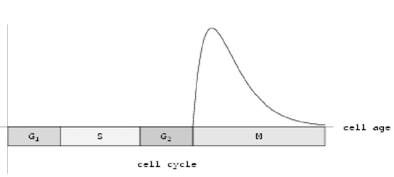
Fig. 1: Schematic of the phases $G_{1}$ (first gap), $S$ (synthesis), $G_{2}$ (second gap), and $M$ (mitosis) of the cell cycle correlated to cell age. The graph over the mitotic phase corresponds to the distribution of cell ages at division (the response of the function $\theta$ to age.)

In the HDC model in [4], the behavior of individual cells is tracked cell by cell on a spatial lattice. This discrete formulation relates detailed information about fundamental processes at the cellular level, such as cell-cell adhesion, entry to and from quiescence, division, apoptosis, and phenotype mutation, to behavior of the tumor mass. In the continuous age-size structured model of this paper, behavior at the population level is also related to behavior at the individual cell level, with cell age and size dependent densities providing the connection to these processes. The use of continuous densities constitutes a local averaging of individual traits.

The dependent variables of the model are:

• $p_{i}(x,a,s,t)$ = density of proliferating tumor cells of type $i$ in the tumor at position $x$, age $a$, and size $s$ at time $t$, where $i=0$ corresponds to a mutated type p53 gene, and $i=1,2,\dots,n$ corresponds to a linear sequence of mutated phenotypes of increasing aggressiveness. The number of mutations can be very large, with successive phenotypes possessing greater proliferative characteristics and capacity for spatial movement.

• $q_{i}(x,a,s,t)$ = density of quiescent tumor cells of type $i$ in the tumor at position $x$, age $a$, size $s$, and mutation phenotype $i=0,2,\dots,n$ at time $t$.

• $f(x,t)$ = surrounding tissue macromolecule (MM) density at position $x$ at time $t$. It is assumed that these macromolecules are distributed heterogeneously in $\Omega$, but immobile in $\Omega$.

• $m(x,t)$ = matrix degradative enzyme (MDE) concentration at position $x$ at time $t$. MDE is produced by the tumor cells and diffuses in $\Omega$.

• $c(x,t)$ = oxygen concentration at position $x$ at time $t$. Oxygen is produced by the extracellular MM, diffuses in $\Omega$, and is consumed by the tumor cells.

• $P(x,t)=\sum_{i=0}^{n}\,\int_{0}^{a_{M}}\int_{s_{m}}^{s_{M}}\,p_{i}(x,a,s,t)\,ds\,da=$ the total population density in $x$ of proliferating cells of all types at time $t$.

• $Q(x,t)=\sum_{i=0}^{n}\,\int_{0}^{a_{M}}\int_{s_{m}}^{s_{M}}\,q_{i}(x,a,s,t)\,ds\,da=$ the total population density in $x$ of quiescent cells of all types at time $t$.

• $N(x,t)=P(x,t)+Q(x,t)=$ total tumor population density in $x$ of all cell types at time $t$.

The equations governing the proliferating-cell densities of the tumor are

$$\frac{\partial}{\partial t}p_{i}(x,a,s,t)= -\,\underbrace{\frac{\partial}{\partial a}p_{i}(x,a,s,t)}_{\mbox{\tiny cell aging}}\,-\,\underbrace{\frac{\partial}{\partial s}(\kappa_{i}(a,s,c)p_{i}(x,a,s,t))}_{\mbox{\tiny cell growth}}$$ (1a)

$$+\underbrace{\nabla\cdot(D_{p_{i}}(x,a,s,N)\nabla p_{i}(x,a,s,t))}_{\mbox{\tiny diffusion}}-\underbrace{\chi_{i}\nabla\cdot(p_{i}(x,a,s,t)\nabla f(x,t))}_{\mbox{\tiny haptotaxis}}$$

$$-\underbrace{\rho_{i}(x,a,s,c,N)p_{i}(x,a,s,t)}_{\mbox{\tiny cell death from insufficient oxygen}}-\underbrace{\theta_{i}(x,a,s,c,N)p_{i}(x,a,s,t)}_{\mbox{\tiny division with sufficient oxygen}}$$

$$-\underbrace{\sigma_{i}(x,a,s,c,N)p_{i}(x,a,s,t)}_{\mbox{\tiny exit to quiescence}}+\underbrace{\tau_{i}(x,a,s,c,N)q_{i}(x,a,s,t)}_{\mbox{\tiny entry from quiescence}},$$

with age-boundary conditions

$$\underbrace{p_{i}(x,0,s,t)}_{\mbox{\tiny newborn type $i$ cells}}= \,4(1\,-\psi_{i}\,)\,\underbrace{\int_{0}^{a_{M}}\theta_{i}(x,a,2s,c,N(x,t))p_{i}(x,a,2s,t)\,da}_{\mbox{\tiny type $i$ cell division}}$$ (1b)

$$+\,4\,\psi_{i-1}\,\underbrace{\int_{0}^{a_{M}}\theta_{i-1}(x,a,2s,c,N(x,t))p_{i-1}(x,a,2s,t)\,da}_{\mbox{\tiny type $i-1$ cell division}},$$

where $\psi_{i}$ is the fraction of type $i$ cells with type $i+1$ mutation. For cells that have undergone only one primary cancer forming mutation (such as a p53 mutation), we set $i=0$ and $\psi_{-1}=0$. The coefficient of 4, rather than the more intuitive splitting value of 2, results from the assumption of even cell division; uneven cell division would require a mitosis kernel and integration over the size variable, $s$, in equation (1b) [59, 62].

The equations governing the quiescent-cell densities are

$$\frac{\partial}{\partial t}q_{i}(x,a,s,t)= -\underbrace{\frac{\partial}{\partial a}q_{i}(x,a,s,t)}_{\mbox{\tiny cell aging}}-\underbrace{\nu_{i}(x,a,s,c,N(x,t))q_{i}(x,a,s,t)}_{\mbox{\tiny cell death from insufficient oxygen}}$$ (1c)

$$+\underbrace{\sigma_{i}(x,a,s,c,N(x,t))p_{i}(x,a,s,t)}_{\mbox{\tiny entry from proliferation}}-\underbrace{\tau_{i}(x,a,s,c,N(x,t))q_{i}(x,a,s,t)}_{\mbox{\tiny exit to proliferation}}.$$

The quiescent-cell populations lack a boundary condition in age since they are ”born” when proliferating cells of the same mutation class become quiescent.

The equations governing tissue macromolecule, matrix degradative enzyme, and oxygen densities are precisely those used in [4]:

$$\frac{\partial}{\partial t}f(x,t)\,=\, -\,\underbrace{\delta m(x,t)f(x,t)}_{\mbox{\tiny degradation}},$$ (1d)

$$\frac{\partial}{\partial t}m(x,t)\,=\, \underbrace{D_{m}\nabla^{2}m(x,t)}_{\mbox{\tiny diffusion}}\,+\,\underbrace{\mu P(x,t)}_{\mbox{\tiny production}}\,-\,\underbrace{\lambda m(x,t)}_{\mbox{\tiny decay}},$$ (1e)

$$\frac{\partial}{\partial t}c(x,t)\,=\, \underbrace{D_{c}\nabla^{2}c(x,t)}_{\mbox{\tiny diffusion}}\,+\,\underbrace{\beta f(x,t)}_{\mbox{\tiny production}}\,-\,\underbrace{\gamma P(x,t)-\eta Q(x,t)}_{\mbox{\tiny uptake}}\,\,-\,\underbrace{\alpha c(x,t)}_{\mbox{\tiny decay}}.$$ (1f)

Equations (1a)-(1f) are combined with initial conditions and no-flux boundary conditions on the boundary $\partial\Omega$ of $\Omega$.

Equation (1a) balances the way cells age, grow, and move in time. The first term on the right-side of equation (1a) accounts for the aging of cells, which is one-to-one with advancing time. In the second term in equation (1a), $\kappa_{i}(a,s,c)$ is the rate at which proliferating cells increase size, i.e., $\int_{s_{1}}^{s_{2}}\frac{1}{\kappa_{i}(a,s,c)}ds$ is the time required for a cell of type $i$ to grow from size $s_{1}$ to size $s_{2}$. The diffusion term in equation (1a) accounts for cell movement due to random motility, interphase drag, the interaction between cells, volume displacement due to cell division, and cell-cell adhesion [10]. The diffusion coefficient $D_{p_{i}}(x,a,s,N(x,t))$ can be allowed to depend on the independent and dependent variables to incorporate mechanistic features of these processes. For example, cells in higher mutation phenotype classes may have smaller cell-cell adhesion properties, and thus have a larger coefficient. Dividing cells of larger size may exert greater force of volume displacement, and thus have a larger coefficient. In equation (1a), the haptotaxis term represents directed movement of cells toward concentrations of MM, which is the source of oxygen necessary for tumor cell growth, and is degraded by tumor cell produced MDE. The coefficient $\rho_{i}(x,a,s,c,N(x,t))$ of proliferating cell loss in equation (1a) is dependent on the density of cells in competition for the supply of oxygen. In equation (1b), $\theta_{i}(x,a,s,c,N(x,t))$ is the rate at which cells of type $i$, age $a$, and size $s$ divide at $x$ per unit time, where it is assumed that a mother cell divides into two daughter cells of equal size (unequal division can also be modeled [62]). The division rate $\theta_{i}(x,a,s,c,N(x,t))$ depends on the age of cells, the supply of oxygen, as well as on the density of cells, with reduced capacity for division as the oxygen supply decreases and the density increases. The negative sign in front of $\theta_{i}(x,a,s,c,N(x,t))$ reflects the loss of cells due to the division process. The mother cell of age $a$ and size $s$ is replaced by two daughter cells, each having age $0$ and half the size of the mother cell, as described in the boundary condition (1b). The coefficients $\sigma_{i}(x,a,s,c,N(x,t))$ and $\tau_{i}(x,a,s,c,N(x,t))$ of transition to and from quiescence in equation (1a) depend on the supply of oxygen and the density of tumor cells. Lower oxygen and higher density results in increased entry to quiescence and higher oxygen and lower density results in increased recruitment from quiescence. The equation (1c) governing the quiescent cells is interpreted similarly, where it is assumed that quiescent cells are not motile. In this model, we represent the properties of individual cell behavior as rates of transition dependent on cell spatial position, age, and size. The inclusion of cell age and size structure allows incorporation of cell level processes without tracking of each cell history, cell by cell (as is done in [4]). The hybrid and continuum modeling approaches have complementarity in development, analysis, and computability, in which advantages of each can be exploited.

2.2 A Simplified Two-Dimensional Model with No Size Structure

The following model is a version of the model above with no size structure, two spatial dimensions (denoted by $(x,y)\in\Omega$), and one compartment each of proliferating- and quiescent-cell types. The equations governing the two classes of cell densities of the tumor are

$$\frac{\partial}{\partial t}p(x,y,a,t)= -\underbrace{\frac{\partial}{\partial a}p(x,y,a,t)}_{\mbox{\tiny cell aging}}$$ (2a)

$$+\underbrace{D_{p}\nabla^{2}p(x,y,a,t)}_{\mbox{\tiny diffusion}}-\underbrace{\chi\nabla\cdot\big{(}p(x,y,a,t)\nabla f(x,y,t)\big{)}}_{\mbox{\tiny haptotaxis}}$$ (2b)

$$-\underbrace{\rho(x,y,a,c)p(x,y,a,t)}_{\mbox{\tiny cell death from insufficient oxygen}}-\underbrace{\theta(x,y,a,c)p(x,y,a,t)}_{\mbox{\tiny division with sufficient oxygen}}$$

$$-\underbrace{\sigma(x,y,a,c,N(x,t))p(x,a,s,t)}_{\mbox{\tiny exit to quiescence}}+\underbrace{\tau(x,y,a,c)q(x,y,a,t)}_{\mbox{\tiny entry from quiescence}},$$

$$\frac{\partial}{\partial t}q(x,y,a,t)= -\underbrace{\frac{\partial}{\partial a}q(x,y,a,t)}_{\mbox{\tiny cell aging}}-\underbrace{\nu(x,y,a,c)q(x,y,a,t)}_{\mbox{\tiny cell death from insufficient oxygen}}$$ (2c)

$$+\underbrace{\sigma(x,y,a,c,N(x,t))p(x,y,a,t)}_{\mbox{\tiny entry from proliferation}}-\underbrace{\tau(x,y,a,c)q(x,y,a,t)}_{\mbox{\tiny exit to proliferation}},$$

with age-boundary conditions

$$\underbrace{p(x,y,0,t)}_{\mbox{\tiny newborn cells}}\,=\,2\underbrace{\int_{0}^{a_{0}}\theta(x,y,a,c)p(x,y,a,t)\ da}_{\mbox{\tiny division rate}}.$$ (2d)

The equations governing tissue macromolecule ($f$), matrix degradative enzyme ($m$), and oxygen ($c$) densities remain as defined in equations (1d)-(1f). All equations are combined with initial conditions and zero flux boundary conditions on an $(x,y)$-rectangle $\Omega$.

3 Computations of Cancer Tumor Invasion

We can demonstrate some aspects of the behavior of the reduced system defined by equations (2b)-(2d) and equations (1d)-(1f) through computations using parameters and functional forms chosen for illustrative purpose rather than biological foundation. Take the spatial domain $\Omega=[-5,5]\times[-5,5]$ and take

$$D_{p}=0.0005,\,\chi=0.01,\,D_{m}=0.01,\,D_{c}=0.05,$$ (3a)

$$\rho(x,y,c)=0.1\,\max\{1.0-c,0\},\,\nu(x,y,c)=2.0\,\max\{1.0-c,0\},$$ (3b)

$$\delta(x,y)=50.0,\,\mu(x,y)=1.0,\,\lambda(x,y)=0.0,\,\beta(x,y)=0.5,$$ (3c)

$$\gamma(x,y)=0.57,\,\eta(x,y)=0.0,\,\alpha(x,y)=0.025,$$ (3d)

$$\sigma(x,y,c)=10.0\,\max\{1.0-c,0\},\,\tau(x,y,c)=2.0\,c.$$ (3e)

The distribution of division ages is assumed to have the form of an offset integrand of the Gamma function (see Figure 1),

$$\theta(x,y,a,c)=\left\{\begin{array}[]{rl}10.0\,c\exp(-10(a-1))\ (2a-1)^{5},&a>0.5,\\ 0,&a<0.5,\end{array}\right.$$ (3f)

where 0.5 is the minimum age at which a cell can divide. The initial conditions are

$$p(x,y,a,0) = 5.0\,G(\sqrt{(x-5)^{2}+(y-5)^{2}},0,0.5),$$ (3g)

$$q(x,y,a,0) = 0.5\,p(x,y,0),$$ (3h)

$$f(x,y,0) = 0.2\,\cos(0.4\,x^{2})\,\sin(0.2\,y^{2})+0.2,$$ (3i)

$$m(x,y,0) = 2.5\,G(\sqrt{(x-5)^{2}+(y-5)^{2}},0,0.5),$$ (3j)

$$c(x,y,0) = 10.0\,f(x,y,0),$$ (3k)

where

$$G(z,z_{\mu},z_{\sigma})=\frac{\exp(-\frac{(z-z_{\mu})^{2}}{2\,z_{\sigma}^{2}})}{\sqrt{2\,\pi}\,z_{\sigma}}.$$

Numerical computations of the proliferating-cell density and macromolecule density for the simplified model are illustrated in Figures 2-4 as snapshots in time. The simulation in Figures 2-4 demonstrates the temporal development of spatial heterogeneity in the tumor mass from a radially symmetric initial condition of tumor cells and heterogeneous initial condition of surrounding macromolecules. The macromolecule tissue is displaced by the tumor tissue as a consequence of haptotactic movement of the tumor cells, driven by the matrix degradative enzyme they produce. The interior core of the tumor mass becomes necrotic, because of its increasing distance from the oxygen supply provided by the macromolecule matrix source. Once aspect of this computation is that the tumor edge consists of an outer layer of proliferating cells and an inner layer of quiescent cells.

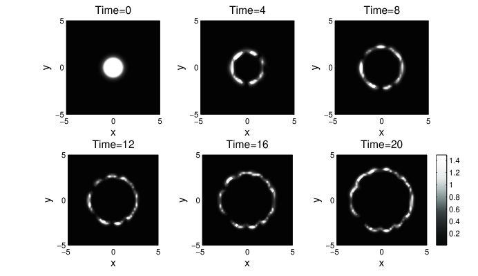
Fig. 2: Proliferating-cell density ($P$) for the system defined by equations (2b)-(2d) and equations (1d)-(1f) . The parameters used in this computation are defined in equations (3a)-(3k).

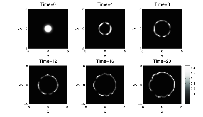
Fig. 3: Quiescent-cell density ($Q$) for the system defined by equations (2b)-(2d) and equations (1d)-(1f) . The parameters used in this computation are defined in equations (3a)-(3k).

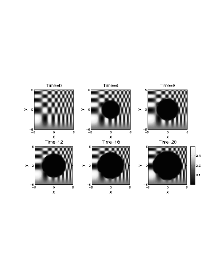
Fig. 4: Macromolecule density ($f$) for the system defined by equations (2b)-(2d) and equations (1d)-(1f) . The parameters used in this computation are defined in equations (3a)-(3k).

4 Computational Methodology

Computational robustness and efficiency is vital for the methods used to solve the high-dimension, multiscale models developed in this paper. The primary issue is the age discretization and how to decouple it from the time discretization without ignoring the fact that age and time advance together. This approach foreshadows how one may wish to handle size structure. The decoupling of the age and time discretizations allows for adaptivity in the time variable; we discuss a particularly effective method for the time integration called step-doubling. The third computational consideration is in how we solve the system in the space variables. We use an alternating direction implicit method, which is a novel approach when incorporated into the step-doubling method for time.

There is a plethora of numerical methods for solving models with just age or size structure [8, 9, 21, 28, 36, 41, 45, 57]. These methods use uniform age and timesteps which are equal to one another in the case of age structure, or do the equivalent in the context of size structure of introducing a new size node at every time step. This approach does not work well for problems with multiple time scales because the fastest time scale tends to be in the spatial variables.

To understand the nature of this problem, consider a fixed, uniform age discretization. Solving the system along characteristics would require the age interval width equal to the time step. This would result in many more age nodes than are needed to accurately solve the problem in the age variable because of the small time step. For size structure, the analogous situation is to introduce many more size nodes at the birth boundary than are needed. An additional concern with size structure is that characteristic curves in the size-time plane can converge, resulting in unnecessarily narrow size intervals. Regridding was used in [57] and [9] to adjust for the effects of narrowing gaps between characteristics, but they do not address the issue of small size nodes at the birth boundary. For example, the method proposed in [9] has an advantage of simplicity – the idea is to merge the narrowest size interval with one of its neighbors after each time step – but is not a satisfactory solution because small size intervals can arise continuously at the birth boundary while elsewhere size intervals continue to narrow due to the nature of the characteristic curves. Moreover, regridding comes at a computational cost. A natural solution to this problem lies in using a finite element space with a moving reference frame in age or size, which is the approach we use in this paper.

Previous numerical methods designed explicitly for models with dependence on age, time and space were developed outside the context of an application and required uniform age and time discretizations with the age step chosen to equal the time step [38, 39, 44]. In contrast, the methods used to obtain the computational results presented in this paper [12, 14] were motivated by models of Proteus mirabilis swarm-colony development where the need to decouple age and time discretizations was clear from the problem [13, 27, 51]. In the process of applying these methods to the system defined in [27], it became clear that the numerical methods and software used previously were not merely inefficient, but also gave qualitatively incorrect answers (although these methods did decouple the age and time discretizations, they did so by not moving the age discretization along characteristics; see the appendix in [13] for a discussion.) This is a critical pitfall to avoid and highlights the importance of using methods with known convergence properties for a particular system.

We use Galerkin finite element methods that use a moving grid to allow for independent, nonuniform age and time discretizations and whose development has focused on robustness as well as computational efficiency. The important property of these methods is that the age step need not equal the time step. Instead, the positions of the age nodes are adjusted by the time step. The methods preserve the important fact that age and time advance together. The methods in [38, 39, 44] also discretized along characteristics, but they did so simultaneously in age and time and thus imposed the often crippling constraint that the time and age steps be both constant and equal. The difficulty with this approach is twofold. First, the use of constant age and time steps prevents adaptivity of the discretization in age or, especially, time. Second, and more importantly, the coupling of the age and time meshes can cause great losses of efficiency since only rarely will the dynamics in time be on the same scale as the dynamics in age. This is particularly the case when space is involved since sharp moving fronts can require small time steps, whereas the behavior in the age variable can remain relatively smooth. The age discretization presented in [38, 39, 44] can be viewed as special cases of the methods presented in [12, 14] by setting the time and age meshes to be constant and equal and using a backward Euler discretization in time and a piecewise constant finite element space in age.

Step-doubling [15, 29, 53] is a conceptually simple, yet quite effective method for the adaptive time integration of differential equations. Over a time step, we compute one solution over the entire time step, and then a second solution over two successive half steps. These two different solutions give us two things. First, we can compare solutions to determine the accuracy of our approximation for the purposes of adaptivity of the time step. Second, we can combine solutions to get a likely second-order accurate approximation, even when each step in the step-doubling process is first-order accurate.

To solve the model equations in the spatial variables, we use an ADI method (also called operator splitting) where we first solve the equations in just the $x$ derivatives and zero-order terms, and then in just the $y$ derivatives [24, 37, 49, 56, 58].

This approach reduces our two-dimensional problem in space to a set of more easily solved one-dimensional spatial problems; we need to solve a series of block tridiagonal linear systems instead of a more computationally expensive wide-banded linear system. Because ADI methods are time ordered, the ADI method needs to be embedded into the step-doubling algorithm.

The combination of these methods results in the following breakdown of the model equations. First, the moving-grid Galerkin methods in age reduce the age-, time-, and space-dependent equations to systems of differential equations that depend on time and two spatial variables. We then solve each of these equations by a combination of step-doubling and ADI methods; we take a step in the $x$ direction and zero-order terms, followed by a step in the $y$-direction, within each substep of step-doubling. This integrated stepping is illustrated in Figure 5.

Fig. 5: Schematic of the combination of the step-doubling and ADI methods to advance the solution of a time and space dependent system from time $t$ to time $t+\Delta t$. The operators $L_{x+0}$ and $L_{y}$ represent the $x$ derivatives plus zero-order terms, and the $y$ derivatives, respectively.

The software used to generate the computed solutions in this paper has a similar structure to BuGS [11]. The age methods presented in [12, 14] use discontinuous piecewise polynomials as basis function for the age space, which results in a distinct system of parabolic partial differential equations for each age interval if we keep time and space continuous. This in turn results in a distinct linear system for each age interval when we fully discretize the equations. In the tumor invasion software, we use piecewise constant functions in age with post-processing to continuous piecewise linear functions. As mentioned above, the tumor invasion software works by updating the age discretization at the beginning of a time step and then applying the step-doubling method to the subsystems corresponding to each age interval splitting the spatial operator into two separate operators over each dimension.

As in BuGS, the tumor invasion software requires the user to define the spatial discretization of the equations by writing a residual function based on first-order backward differences in time. The software then uses the implementation of the step-doubling method described in [15] to get a second-order accurate in time implicit finite difference scheme. The software also features step control for the convergence of Newton’s method and automatic approximation of the Jacobi matrix.

5 Conclusions and Further Research

In this paper we presented physiologically and spatially structured continuous deterministic models of cancer tumor invasion. We presented a general model whose equations depend on variables representing size, age, space and time. We then treated a simplified model without size structure and with only two spatial dimensions. The simplified model contained one mutation class of proliferating and quiescent cells. The aim of this approach is to move tumor invasion modeling away from phenomenological models toward more mechanistic, biologically informed, and reliably predictive models. These more complex models required a more sophisticated computational methodology to investigate numerically the computationally intensive model equations.

The most immediate extension of this work is to determine the models parameters and functional forms from biological data and experiments. The current methodology and software is sufficient to handle multiple mutation classes of proliferating and quiescent cells, but a deeper understanding of the biology is needed to benefit from this extension. Computational results from more biologically detailed models are expected, in turn, to contribute to a deeper understanding of the underlying biology.

The most important mathematical extension of the methodology is to develop size-time finite elements to handle size-structured equations. Rather than being developed for general forms of transport, extensions of the existing methods for age structure to size structure will use the specific nature of physiological change in tumor cells to allow the incorporation of size structure into a model at a low cost in terms of computational resources. Anticipated complications in handling size structure include birth in a size-structured context with respect to both the numerical methods and their analyses. Since the characteristic curves in the size-time plane are no longer lines with slope one, as was the case for age structure, some important questions are: what types of characteristic curves should we consider and how do we handle situations where these curves become asymptotically close within the moving grid framework? What happens if they meet and shocks form?

Two immediate concerns must be addressed for the problem of size dependence in tumor invasion models. The first issue is the introduction of new size nodes at the birth boundary, and the second is the handling of size intervals that contract due to the convergence of size-time characteristic curves. We expect the major complication in the size nodes to occur when growth slows as cells reach a certain size. However, because of the nonlinearities in the problem, it is insufficient to merely assume that a size interval will strictly decrease length. Addressing these two concerns will lay the foundation for methods that handle more complicated characteristics, including the formation of shocks that can form in situations where growth has complex dependencies on the physiological traits of an individual as well as the external environment.

As in the methods for age-structured systems, the moving grid formulation is expected to account for the growth of individuals, taking the place of direct differencing of the size variable. And as in the case of age structure, the use of a space of discontinuous piecewise polynomials as the basis functions in size is expected to allow each size interval to be treated with a separate linear system. If the system has dependence on both age and size, we would have a two dimensional array of independent linear systems at each time step.

An important benefit of using size-time Galerkin finite elements is having one mathematical framework define many methods with higher-order accuracy. Because of the need to keep computational costs down in each dimension of the high-dimension systems under study, without sacrificing robustness, the ability to choose the order of convergence of the method is quite useful.

A major extension of the software and methodology is to add a third space dimension through an additional sub-operator in the ADI method. This methodology for handling three space dimensions is expected to be sufficient for generating initial results that aim to extend our understanding of tumor invasion beyond the 2D-space models. Other ADI methods that may work within this framework are Douglas-Gunn [58] and Strang Splitting [56].

Although we have provided a specific mathematical treatment of the spatial dynamics of tumor invasion, we remark that modeling spatial dynamics can be more complicated in biological systems than in physical systems. A broad examination of different modeling approaches is required, including the continuous approach in this paper, and how it relates to other approaches, such as the hybrid discrete-continuous formulation discussed in [4]. Multiscale models of the type considered in this paper have different time scales for the dynamics at the different physical scales. For example, in the system defined in equations (1a)-(1f), the cellular scale gives rise to time scales in the age and size variables, whereas the tumor scale gives rise to a different time scale in the spatial variables. Independent of the specific type of spatial representation used, decoupling time from age or size is critical for effective solution of the model equations.

Many of the features of the cancer models, such as taxis, aging and growth, are seen in other biological systems; prior work on Proteus mirabilis swarm-colony development is but one example [13]. Biological systems abound where either spatial dynamics induce the behavior of interest, or where the spatial dynamics is the behavior of interest. In the same manner, the behavior of interest in a biological system can depend on the distribution of physiological traits such as age or size, or those distributions are the topic of interest. We hope that the methodology presented in this paper will provide a template for handling a broader range of biological problems.

References

- [1] J. A. Adam and N. Bellomo, eds., A Survey of Models for Tumor-Immune System Dynamics, Modelling and Simulation in Science, Engineering, and Technology, Birkhäuser, Boston, 1997.
- [2] A. R. A. Anderson, The effects of cell adhesion on solid tumour geometry, in Morphogenesis and Pattern Formation in Biological Systems, T. Sekimura, S. Noji, N. Ueno, and P. Maini, eds., Springer-Verlag, 2003, pp. 315–325.
- [3] , Solid tumour invasion: The importance of cell adhesion, in Function and Regulation of Cellular Systems: Experiments and Models, part VII, A. Deutsch, M. Falcke, J. Howard, and W. Zimmermann, eds., Birkhäuser, 2003, pp. 379–389.
- [4] , A hybrid mathematical model of solid tumour invasion: The importance of cell adhesion, Math. Med. Biol. IMA Journal, in press (2005).
- [5] A. R. A. Anderson and M. A. J. Chaplain, Continuous and discrete mathematical models of tumour-induced angiogenesis, Bull. Math. Biol., (1998).
- [6] A. R. A. Anderson, M. A. J. Chaplain, E. L. Newman, R. J. C. Steele, and A. M. Thompson, Mathematical modelling of tumour invasion and metastasis, J. Theoret. Med., 2 (2000).
- [7] A. R. A. Anderson and A. W. Pitcairn, Application of the hybrid discrete-continuum technique, in Polymer and Cell Dynamics, Part III, W. Alt, M. Chaplain, M. Griebel, and J. Lenz, eds., Birkhäuser, 2003, pp. 261–279.
- [8] O. Angulo and J. C. López-Marcos, Numerical schemes for size-structured population equations, Math. Biosci., 157 (1999), pp. 169–188.
- [9] , Numerical integration of fully nonlinear size-structured population models, Appl. Numer. Math., 50 (2004), pp. 291–327.
- [10] R. P. Araujo and D. L. S. McElwain, A history of the study of solid tumor growth: The contribution of mathematical modelling, Bull. Math. Biol., 66 (2004), pp. 1039–1091.
- [11] B. P. Ayati, 1.0 user guide, Tech. Report CS-96-18, University of Chicago, 1996.
- [12] , A variable time step method for an age-dependent population model with nonlinear diffusion, SIAM J. Numer. Anal., 37 (2000), pp. 1571–1589.
- [13] , An age- and space-structured model of Proteus mirabilis swarm-colony development, Tech. Report 2004-04 (arXiv:q-bio.CB/0412003), SMU Mathematics Dept., http://arxiv.org/abs/q-bio/0412003, 2004.
- [14] B. P. Ayati and T. F. Dupont, Galerkin methods in age and space for a population model with nonlinear diffusion, SIAM J. Numer. Anal., 40 (2002), pp. 1064–1076.
- [15] , Convergence of a step-doubling Galerkin method for parabolic problems, Math. Comp., 74 (2005), pp. 1053–1065. Article electronically published on September 10, 2004.
- [16] N. Bellomo and L. Preziosi, Modelling and mathematical problems related to tumor evolution and its interaction with the immune system, Mathematical and Computer Modelling, 32 (2000), pp. 413–452.
- [17] A. Bertuzzi, A. D’Onofrio, A. Fasano, and A. Gandolfi, Modelling cell populations with spatial structure: Steady state and treatment-induced evolution of tumour cords, Discrete and Continuous Dynamical Systems-Series B, 4 (2004), pp. 161–186.
- [18] A. Bertuzzi, A. Fasano, A. Gandolfi, and D. Marangi, Cell kinetics in tumor cords studied by a model with variable cell cycle length, Math. Biosci., 177-178 (2002), pp. 103–125.
- [19] A. Bertuzzi and A. Gandolfi, Cell kinetics in a tumor cord, J. Theo. Biol., 204 (2000), pp. 587–599.
- [20] S. Busenberg and M. Iannelli, A class of nonlinear diffusion problems in age-dependent population dynamics, Nonlin. Anal. Th. Meth. Appl., 7 (1983), pp. 501–529.
- [21] C. Chiu, A numerical method for nonlinear age dependent population models, Diff. Int. Eqns., 3 (1990), pp. 767–782.
- [22] G. di Blasio, Non-linear age-dependent population diffusion, J. Math. Bio., 8 (1979), pp. 265–284.
- [23] G. di Blasio and L. Lamberti, An initial-boundary problem for age-dependent population diffusion, SIAM J. Appl. Math., 35 (1978), pp. 593–615.
- [24] J. Douglas, Jr. and T. Dupont, Alternating-direction galerkin methods on rectangles, in Numerical Solution of Partial Differential Equations - II, Academic Press, New York and London, 1971, pp. 133–213.
- [25] J. Dyson, R. Villella-Bressan, and G. F. Webb, Asynchronous exponential growth in an age structured population of proliferating and quiescent cells, Math. Biosci., 177-178 (2002), pp. 73–83.
- [26] , The evolution of a tumor cord cell population, Communications on Pure and Applied Analysis, (2004).
- [27] S. E. Esipov and J. A. Shapiro, Kinetic model of Proteus mirabilis swarm colony development, J. Math. Biol., 36 (1998), pp. 249–268.
- [28] G. Fairweather and J. C. López-Marcos, A box method for a nonlinear equation of population dynamics, IMA J. Numer. Anal., 11 (1991), pp. 525–538.
- [29] C. W. Gear, Numerical Initial Value Problems in Ordinary Differential Equations, Prentice–Hall, New Jersey, 1971.
- [30] M. E. Gurtin, A system of equations for age-dependent population diffusion, J. Theor. Biol., 40 (1973), pp. 389–392.
- [31] M. E. Gurtin and R. C. MacCamy, Non-linear age-dependent population dynamics, Arch. Rat. Mech. Anal., 54 (1974), pp. 281–300.
- [32] , Diffusion models for age-structured populations, Math. Biosci., 54 (1981), pp. 49–59.
- [33] M. Gyllenberg and G. F. Webb, A nonlinear structured population model of tumor growth with quiescence, J. Math. Biol., 28 (1990), pp. 671–694.
- [34] M. A. Horn and G. F. Webb, eds., Mathematical Models in Cancer, vol. 4 of Discrete Contin. Dyn. Syst. Ser. B, Papers from the workshop held at Vanderbilt University, Nashville, TN, May 3–5, 2002, 2004.
- [35] C. Huang, An age-dependent population model with nonlinear diffusion in , Quart. Appl. Math., 52 (1994), pp. 377–398.
- [36] K. Ito, F. Kappel, and G. Peichl, A fully discretized approximation scheme for size-structured population models, SIAM J. Numer. Anal., 28 (1991), pp. 923–954.
- [37] K. H. Karlsen, K.-A. Lie, J. R. Natvig, H. F. Nordhaug, and H. K. Dahle, Operator splitting methods for systems of convection-diffusion equations: Nonlinear error mechanisms and correction strategies, J. Comp. Phys., 173 (2001), pp. 636–663.
- [38] M.-Y. Kim, Galerkin methods for a model of population dynamics with nonlinear diffusion, Num. Meth. Part. Diff. Eqns., 12 (1996), pp. 59–73.
- [39] M.-Y. Kim and E.-J. Park, Mixed approximation of a population diffusion equation, Computers Math. Applic., 30 (1995), pp. 23–33.
- [40] K. Kubo and M. Langlais, Periodic solutions for a population dynamics problem with age-dependence and spatial structure, J. Math. Biol., 29 (1991), pp. 363–378.
- [41] Y. Kwon and C.-K. Cho, Second-order accurate difference methods for a one-sex model of population dynamics, SIAM J. Numer. Anal., 30 (1993), pp. 1385–1399.
- [42] M. Langlais, A nonlinear problem in age-dependent population diffusion, SIAM J. Math. Anal., 16 (1985), pp. 510–529.
- [43] , Large time behavior in a nonlinear age-dependent population dynamics problem with spatial diffusion, J. Math. Biol., 26 (1988), pp. 319–346.
- [44] L. Lopez and D. Trigiante, A finite difference scheme for a stiff problem arising in the numerical solution of a population dynamic model with spatial diffusion, Nonlin. Anal. Th. Meth. Appl., 9 (1985), pp. 1–12.
- [45] J. C. López-Marcos, An upwind scheme for a nonlinear hyperbolic integro-differential equation with integral boundary condition, Computers Math. Applic., 22 (1991), pp. 15–28.
- [46] R. C. MacCamy, A population model with nonlinear diffusion, J. Diff. Eqns., 39 (1981), pp. 52–72.
- [47] P. Marcati, Asymptotic behavior in age-dependent population dynamics with hereditary renewal law, SIAM J. Math. Anal., 12 (1981), pp. 904–916.
- [48] A. G. McKendrick, Applications of mathematics to medical problems, Proc. Edin. Math. Soc., 44 (1926), pp. 98–130.
- [49] R. I. McLachlan and G. R. W. Quispel, Splitting methods, Acta Numerica, 11 (2002), pp. 341–434.
- [50] L. Preziosi, ed., Cancer Modelling and Simulation, Chapman & Hall/CRC, 2003.
- [51] O. Rauprich, M. Matsushita, K. Weijer, F. Siegert, S. E. Esipov, and J. A. Shapiro, Periodic phenomena in Proteus mirabilis swarm colony development, J. Bacteriol., 178 (1996), pp. 6525–6538.
- [52] M. Rotenberg, Theory of population transport, J. Theor. Biol., 37 (1972), pp. 291–305.
- [53] L. F. Shampine, Local error estimation by doubling, Computing, 34 (1985), pp. 179–190.
- [54] F. R. Sharpe and A. J. Lotka, A problem in age-distribution, Philos. Mag., 21 (1911), pp. 435–438.
- [55] J. G. Skellam, Random dispersal in theoretical populations, Biometrika, 38 (1951), pp. 196–218.
- [56] G. Strang, On the construction and comparison of difference schemes, SIAM J. Numer. Anal., 5 (1968), pp. 506–517.
- [57] D. Sulsky, Numerical solution of structured population models, I. age structure, J. Math. Biol., 31 (1993), pp. 817–839.
- [58] J. W. Thomas, Numerical Partial Differential Equations: Finite Difference Methods, vol. 22 of Texts in Applied Mathematics, Springer-Verlag, New York, 1995.
- [59] S. L. Tucker and S. O. Zimmerman, A nonlinear model of population dynamics containing an arbitrary number of continuous structure variables, SIAM J. Appl. Math., 48 (1988), pp. 549–591.
- [60] G. F. Webb, An age-dependent epidemic model with spatial diffusion, Arch. Rational Mech. Anal., 75 (1980/81), pp. 91–102.
- [61] G. F. Webb, Theory of Nonlinear Age–dependent Population Dynamics, vol. 89 of Pure and Applied Mathematics, Marcel Dekker, New York, 1985.
- [62] G. F. Webb, - and -curves, sister-sister and mother-daughter correlations in cell population dynamics, Computers Math. Appl., 18 (1989), pp. 973–984.