Probabilistic methods for predicting protein functions in protein-protein interaction networks

Abstract

We discuss probabilistic methods for predicting protein functions from protein-protein interaction networks. Previous work based on Markov Randon Fields is extended and compared to a general machine-learning theoretic approach. Using actual protein interaction networks for yeast from the MIPS database and GO-SLIM function assignments, we compare the predictions of the different probabilistic methods and of a standard support vector machine. It turns out that, with the currently available networks, the simple methods based on counting frequencies perform as well as the more sophisticated approaches.

1 Introduction

Large-scale comprehensive protein-protein interaction data, which have become available recently, open the possibility of deriving new information about proteins from their associations in the interaction graph. In the following, we discuss and compare several probabilistic methods for predicting protein functions from the functions of neighboring proteins in the interaction graph.

In particular, we compare two recently published methods that are based on Markov Random Fields [1, 2] with a prediction based on a machine-learning appproach using maximum-likelihood parameter estimation. It turns out that all three approaches can be considered different versions of each other using different approximations. The main difference between the Markov Random Field (MRF) and the machine-learning methods is that the former apprach takes a global look at the network, while the latter considers each networks node as an independent training example. However, in the mean-field approximation required to make the MRF approach numerically tractable, it is reduced to considering each node independently. The local enrichment-method considered in [1] can then be interpreted as another approximation which enables us to make predictions directly from observer frequencies, bypassing the numerical minimization step required in the more general machine-learning approach.

We also extend these methods by considering a non-linear generalization for the probability distribution in the machine-learning approach, and by taking larger neighborhoods in the network into account. Finally, we compare the performance of these methods to a standard Supper Vector Machine.

2 Methods

We consider a network specified by a graph whose nodes are proteins and whose undirected vertices indicate interactions between the proteins. Each node is assigned one of a set of protein functions. In a machine-learning approach to prediction, this assignment follows a simple probability function depending on the protein functions in the network neighborhood of each node and parametrized by a small set of parameters. The learning problem is to estimate these parameters from a given sample of assignments. The prediction can then be performed by evaluating the probability distribution using these parameters.

2.1 Machine-learning approach

Assume we only consider a single protein function at a time. Node assignments can then be chosen binary, $x\in\{0,1\}$, with $1$ indicating that a node has the function under consideration. In the simplest case, the probability that a node $i$ has assignment $x$ depends only its immediate neighbors, and since all vertices of the graph are equal, it can only depend on the number of neighbors $C$, and the number of active neighbors $N$. Borrowing from statistical mechanics, we write the probability using a potential $U(x;C,N)$

$$p(x|C,N)=\frac{e^{-U(x;C,N)}}{Z(C,N)},\qquad Z(C,N)=\sum_{y=0,1}e^{-U(y;C,N)}$$ (1)

where the partition sum $Z(C,N)$ is a normalizing factor. This equation basically expresses that the log-probabilities of $x$ are proportional to the potential $U(x;C,N)$. In a lowest-order approximation, we can choose a linear function for the potential:

$$U(x;C,N;\alpha)=(\alpha_{0}+\alpha_{1}C+\alpha_{2}N)x\quad.$$ (2)

Later, we will extend this approach to more general functions.

The parameters $\alpha$ can be estimated from a set of training samples $(x_{i},C_{i},N_{i})$ by maximum-likelihood estimation. In this approach, they are chosen to maximize the joint probability

$$P=\prod_{i}p(x_{i}|C_{i},N_{i})$$ (3)

of the training data, or equivalently, to minimize its negative logarithm

$$-\log P=\sum_{i}\left[\ln Z(C_{i},N_{i})+U(x_{i};C_{i},N_{i})\right]\quad.$$ (4)

Taking the partial derivative w.r.t. to a parameter gives the equation

$$-\frac{\partial P}{\partial\alpha}=\sum_{i}\left\{-\frac{1}{Z(C_{i},N_{i})}\sum_{y=0,1}\frac{\partial U(y,C_{i},N_{i})}{\partial\alpha}e^{-U(y,C_{i},N_{i})}+\frac{\partial U(x_{i},C_{i},N_{i})}{\partial\alpha}\right\}\quad.$$ (5)

The first term in the bracket is the expectation value of $\partial U/\partial\alpha$ in the neighborhood $(C_{i},N_{i})$ under the probability distributions parametrized by $(\alpha,\ldots)$:

$$\left\langle\frac{\partial U(y,C_{i},N_{i})}{\partial\alpha}\right\rangle_{N_{i},C_{i};\alpha,\ldots}=\frac{1}{Z(C_{i},N_{i})}\sum_{y=0,1}\frac{\partial U(y,C_{i},N_{i})}{\partial\alpha}\,e^{-U(y,C_{i},N_{i})}$$ (6)

At the extremum, the derivative vanishes and we have the simple relation

$$\sum_{i}\left\langle\frac{\partial U(y,C_{i},N_{i})}{\partial\alpha}\right\rangle=\sum_{i}\frac{\partial U(x_{i},C_{i},N_{i})}{\partial\alpha}\quad.$$ (7)

Thus, in the maximum-likelihood model, the parameters are adjusted so that the average expectation values of the derivatives of the potential are equal to the averages observed in the training data. Using eq. 2, this gives the set of three equations.

$$\sum_{i}\left\{\begin{array}[]{l}1\\ C_{i}\\ N_{i}\end{array}\right\}\,\langle x\rangle = \sum_{i}\left\{\begin{array}[]{l}1\\ C_{i}\\ N_{i}\end{array}\right\}\,x_{i}$$ (14)

where the expectation value of $x$ in the environment $(C_{i},N_{i})$ and in the model parametrized by $\alpha$ is given by

$$\langle x\rangle=\langle x\rangle_{\alpha_{0},\alpha_{1},\alpha_{2};C_{i},N_{i}}=\frac{e^{-(\alpha+\alpha_{1}C_{i}+\alpha_{2}N_{i})}}{1+e^{-(\alpha+\alpha_{1}C_{i}+\alpha_{2}N_{i})}}\quad.$$ (15)

Only in the simplest case, $\alpha_{1}=\alpha_{2}=0$, this equation can be solved analytically, leading to the relation:

$$\alpha=\frac{\bar{x}}{1-\bar{x}},\qquad\mbox{with}\qquad\bar{x}=\frac{1}{n}\sum_{i=1}{n}x_{i}\quad.$$ (16)

In the general case, we solve these equations numerically using a conjugate-gradient method by explicitly minimizing the joint probability $P$.

2.2 Network approach

An alternative approach to prediction starts out from considering a given network and the protein function assignments as a whole and assigning a score based on how well the network and the function assignments agree. In the approach of [2], each link contributes to this score with a gain $G_{0}$ or $G_{1}$, resp., if both nodes at the ends of the link have the same function $0$ or $1$, and a penalty $P$ if they have different function assignments. Assuming again that the log-probabilities are proportional to the scores, this induces a probability distribution over all joint function assignments ${\bf x}$ given by

$$p({\bf x})=\frac{1}{Z}e^{-U({\bf x})}\quad,\qquad Z=\sum_{\bf x}e^{-U({\bf x})}$$ (17)

where now the normalization factor is calculated by summing over all possible joint function assignments of the nodes.

The scoring function $U({\bf x})$ can be expressed as

$$U({\bf x}) = -\frac{G_{1}}{2}\sum_{i,j:(i,j)\in E}x_{i}x_{j}-\frac{G_{0}}{2}\sum_{i,j:(i,j)\in E}(1-x_{i})\,(1-x_{j})$$

$$+\frac{P}{2}\sum_{i,j:(i,j)\in E}\left((1-x_{i})\,x_{j}+x_{i}\,(1-x_{j})\right)+\eta_{0}\sum_{i}x_{i}$$

$$= \eta_{0}\sum_{i}x_{i}+\eta_{1}\sum_{i}C_{i}x_{i}+\frac{\eta_{2}}{2}\sum_{i,j:(i,j)\in E}x_{i}x_{j}$$

with the parameters

$$\eta_{2}=-G_{1}-G_{0}-2P\qquad\mbox{and}\qquad\eta_{1}=G_{0}+P\quad.$$ (19)

In terms of statistical mechanics, this describes a ferromagnetic system where the inverse temperature is determined by $\eta_{2}$ and an external field by $\eta_{0}$ and $\eta_{1}$.

Again, maximum-likelihood parameter estimation is performed by finding a set of parameters $\eta=(\eta_{0},\eta_{1},\eta_{2})$ such that the probability of the $N$ sample configurations ${\bf x}^{(n)}$ is maximized:

$$\alpha=\mathop{\rm argmax}_{\alpha}\sum_{n}^{N}\ln p({\bf x}^{(n)};\alpha)=\mathop{\rm argmin}_{\alpha}\left(\sum_{n}U({\bf x}^{(n)})+N\ln Z(\alpha)\right)$$ (20)

The logarithm of the partition sum appearing in the second term can be related to the entropy by

$$S = -\sum_{x}p(x)\,\ln p(x)=\sum_{x}p(x)\,U(x)+\ln Z$$ (21)

$$\Rightarrow\qquad-\ln Z = \langle U\rangle-S=F$$ (22)

The quantity $\langle U\rangle-S$ is the thermodynamical free energy. Maximum likelihood parameters estimation therefore corresponds to choosing the parameters such that the energy of the given configuration is minimized while the free energy of the system as a whole is maximized:

$$\mathop{\rm argmin}_{\alpha}\left(U(X;\alpha)-F(\alpha)\right)=\mathop{\rm argmin}_{\alpha}\left(U(X;\alpha)-\langle U\rangle(\alpha)+S(\alpha)\right)\quad.$$ (23)

Unfortunately, this requires the calculation of both the internal energy, $\langle U\rangle(\alpha)$, and the entropy, $S(\alpha)$, of the system and thus more or less a complete solution of the system.

This can be avoided by employing the mean field approximation, in which the probability distribution $p(x)$ is replaced by a trial distribution $p_{\rm trial}(x)$ as a product of single-variable distributions

$$p_{\rm trial}(x)=p_{1}(x_{1})\ldots p_{n}(x_{n})$$ (24)

which can be completely parametrized by the expectation values $\bar{x}_{i}$ using

$$p_{i}(x_{i})=x_{i}\bar{x}_{i}+(1-x_{i})(1-\bar{x}_{i})=\left\{\begin{array}[]{ll}1-\bar{x}_{i}&\mbox{if $x_{i}=0$}\\ \bar{x}_{i}&\mbox{if $x_{i}=1$}\end{array}\right.$$ (25)

Optimum values for the parameters $\bar{x}_{i}$ can then be estimated by minimizing the KL entropy of $p_{\rm trial}(x)$ vs. the true distribution $p(x)$.

Interestingly, this approximation removes the distinguishing feature of the network approach, namely that the neighborhood structure (in the sense of neghbors of neighbors) is taken into account. The resulting equations are very similar to the machine-learning equations in which neighbors are treated as unrelated.

2.3 Binomial-neighborhood approach

The binomial-neighborhood approach [1] is a simpler approach in which the probability distribution $p(x|C,N)$ is chosen in such a way that it can be directly derived from observed frequencies without the minimization process typical for maximum-likelihood approaches. It is based on the assumption that the distribution of active neighbors $N_{i}$ of a node $i$ follows a binomial distribution whose single probability $p$ depends on whether the node $i$ is active or not:

$$p(N_{i}|C_{i},x_{i}=1)=\left(\begin{array}[]{c}C_{i}\\ N_{i}\end{array}\right)\,p_{1}^{N_{i}}(1-p_{1})^{C_{i}-N_{i}}\quad,$$ (26)

and correspondingly for $x_{i}=0$ using a single probability $p_{0}$. This is the assumption of local enrichment, i.e. that the probability $p_{1}$ to find an active node around another active node is larger than the probability $p_{0}$ to find an active node around an inactive node. Using Bayes’ theorem, we can use this to calculate the probability distribution of $x_{i}$:

$$p(x_{i}|C_{i},N_{i})=\frac{p(N_{i}|C_{i},x_{i})\,p(x_{i}|C_{i})}{p(N_{i}|C_{i})}$$ (27)

where $p(x_{i}|C_{i})=\bar{x}$ is the overall probability of observing an active node, and

$$p(N_{i}|C_{i})=\bar{x}p(N_{i}|C_{i},x_{i}=1)+(1-\bar{x})p(N_{i}|C_{i},x_{i}=0)\quad.$$ (28)

The resulting probability distribution can be written as

$$p(x_{i}=1|C_{i},N_{i})=\frac{\lambda}{1+\lambda}\qquad\mbox{and}\qquad p(x_{i}=0|C_{i},N_{i})=\frac{1}{1+\lambda}$$ (29)

with

$$\lambda=\frac{\bar{x}}{1-\bar{x}}\,\frac{p_{1}^{N_{i}}\,(1-p_{1})^{C_{i}-N_{i}}}{p_{0}^{N_{i}}\,(1-p_{0})^{C_{i}-N_{i}}}\quad.$$ (30)

This can be easily rewritten in the same form as (1)

$$p(x_{i}|C_{i},N_{i})=\frac{1}{Z}\exp\left[-\left(-\ln\frac{\bar{x}}{1-\bar{x}}-\ln\frac{p_{1}}{p_{0}}N_{i}+\ln\frac{1-p_{0}}{1-p_{1}}\,(C_{i}-N_{i})\right)\,x_{i}\right]$$ (31)

The first term in the potential has the same form as (16) and adjusts the overall number of positive sites; the two other terms constitute a bones for having positive neighbors (proportional to $N_{i}$) and a penalty for having negative neighbors (proportional to $C_{i}-N_{i}$).

This approach evidently gives a conditional probability distribution $p(x_{i}|C_{i},N_{i})$ of the same for as the one in the machine-learning approach. However, the coefficient in the potential can be directly calculated from the observed frequencies $\bar{x}$, $p_{0}$, and $p_{1}$. This is only possible because we made here the assumption that the probability distribution $p(N_{i}|C_{i},x_{i})$ is binomial. The machine-learning approach is more flexible in that in does not have to make this assumption and yields a true maximum-likelihood estimate even for distributions that deviate greatly from binomial form. In particular, the binomial distribution implies that the neighbors of a node behave statistically independent, which might be violated in a densely connected network, where we would expect clusters to form.

3 Results

To compare the different prediction methods, we chose the MIPS protein-protein interaction database for Saccharomyces cerevisiae [5, 4] and the GO-SLIM database of protein function assignments from the Gene Ontology Consortium [6]. The latter is a slimmed-down subset of the full gene ontology assignments comprising 32 different processes, 21 functions, and 22 cell compartments. We focused here on the process assignments as these were expected to correspond most closely to the interaction network.

We compared four methods:

1. the binomial neighborhood enrichment from sec. 2.3,

2. the machine-learning maximum-likelihood method from sec. 2.1 using a linear potential (2)

3. the same method with an extended non-linear potential, and

4. a standard support vector machine [7].

For the probabilistic methods, we first looked at the single-function prediction problem in which the system is presented with a binary assignment expressing which proteins are known to have a given function, and then makes a prediction for an unknown protein based on the number of neighbors that have this function.

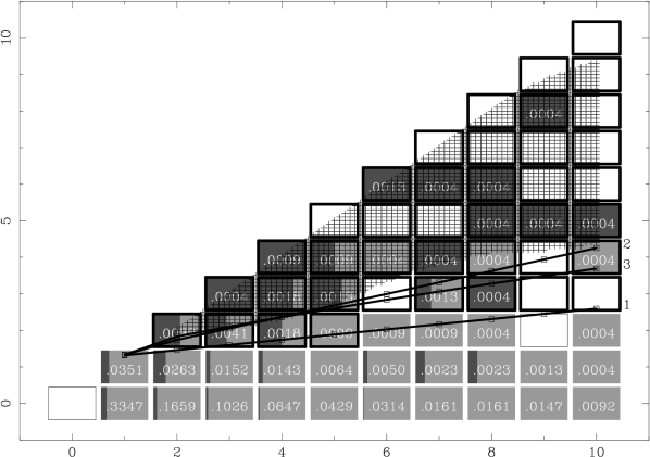
Figure 1: Glyph plot summarizing the probability distribution for a single-function prediction problem. Each box represents a possible situation of a single node, characterized by the total number of neighbors on the $x$-axis, and the number of neighbors having the funtion of interested on the $y$-axis. The numbers indicate the total incidence of the situation, while the shading expresses how frequently the central node had the function of interest in that situation. The lines are the decision boundaries for the binomial method and the linear and polynomal machine-learning methods. The shading is the prediction region from the SVM.

In this case, the local environment of a node can be described by two numbers: $n$, the number of neighbors, and $j$, the number of neighbors that have the function assignment under consideration. The content of the training data set can be characterized by a glyph plot such as in fig. 1.

After learning the training data, the probabilistic method has inferred a probability distribution that yields, for each pair $(n,j)$, a probability $p(X_{i}=1|n,j)$ which is then utilized for predictions. The 50%-level of this probability, which determines the prediction in a binary system, is indicated in fig. 1 by green lines.

The three probabilistic predictors in fig. 1 yield similar results that differ rarely by more than one box. The main difference is that the binomial predictor is restricted to a straight line, while the linear and non-linear maximum-likelihood predictors can accomodate a little turn. Linear and non-linear predictors differ only minimally.

Figure 2: Sensitivity-specificity curve for the three probabilistic prediction methods for a single-function prediction.

Finally the prediction from a support vector machine that was trained on the same single-function data set is indicated by a shaded area marking all those $(n,j)$ for which the SVM returned a positive prediction. The border of this area very closely follows the linear and non-linear M.L. predictors.

Fig. 2 shows a sensitivity-specificity curve using five-fold cross validation for single-function prediction using the probabilistic predictors. Again, all three curves follow each other quite closely, with a slight edge for the nonlinear M.L. predictor.

The preceding discussion applied to the problem of single function prediction. To perform full prediction, we generated each of the three predictors separately for each function and chose, for each protein with an unknown function, the prediction with the largest probability. For simplicity, this approach does not take into account possible correlations between different protein functions. However, such correlations were taken into account for the support vector machine, which generated a full set of cross-predictors (predicting function $i$ with neighbors of type $j$).

Figure 3: Accuracy of multiple-function prediction as a function of the number of predictions made using the three probabilistic prediction methods.

In the probabilistic case, each predictor does not only provide us with a yes-no decision, but also with a probability for the prediction. We can use the information to restrict the predictions to highly probable ones. Fig. 3 shows the accuracy of the prediction as a function of how many predictions are made with different cut-offs in the predicted probability. Again, all three curves closely follow each other, with maybe a small but unsignificant edge of the linear M.L. predictor. The predictions from all predictors including the SVM were similar, and combining them would not have improved predictive accuracy.

METHOD	#SUCCESS	accuracy
binomial classifier	623	31%
linear M.L. classifier	655	33%
nonlinear M.L. classifier	640	31.7%
linear SVM classifier	601	29.8%
randomized network	101	11.4%
binomial classifier, process		32.5%
randomized network		8.7%

Table 1: Prediction accuracy in five-fold cross validation for the yeast data set.

Finally, the success rates for all predictors are shown in table 1 using five-fold cross-validation on a data set of 2014 unique function assignments for the yeast proteome. It turns out that all four methods perform closely, with success rates between 30 and 33%. This compares to the null-hypothesis of prediction in a randomized network, in which we would have a success rate of 11% for these data. The protein-protein interaction data therefore roughly triples the prediction success over a random network. However, all methods, from the simple, counting-based binomial classifier to the full support vector machine, perform similarly.

We also extended our methods to take larger neighborhoods (second and higher-order neighbors) into account, but failed to substantially improve predictive power.

Finally, we also performed protein function prediction on a recently published protein-interaction network for Drosophila melanogaster [3], with similar results.

4 Discussion

We compared different probabilistic approaches to predicting protein functions in protein interaction networks. Under closer analysis, the different Markov Random Field methods in the literature can be related to a basic machine-learning approach with maximum-likelihood parameter estimation. Using real data, they exhibit similar performance, with simple methods performing as well as more complex ones. This might indicate limits on the functional information contained in protein-protein interaction networks.

A standard support vector machine gave similar result, though it was equipped with more information, namely the frequencies of all function classes in the neighborhood. The additional information did neither improve nor harm predictive performance.

References

- [1] S. Letovsky, S. Kasif, Bioinformatics 19, Suppl. 1, i197 (2003).
- [2] M. Deng, T. Chen, F. Sun, in: Proceedings, RECOMB ’03, 7th international conference on Research in Computational Molecular Biology, p. 95, ACM Press, New York, NY (2003).
- [3] L. Giot et. al., Science 302, 1727 (2003).
- [4] P. Uetz et. al., Nature 403, 623 (2000).
- [5] H. W. Mewes et. al., Nucleic Acids Research 32, D41 (2004).
- [6] The Gene Ontology Consortium, Nucleic Acids Res 32, D258 (2004).
- [7] C.-C. Chang, C.-J. Lin, LIBSVM : a library for support vector machines, 2001. Software available at http://www.csie.ntu.edu.tw/ cjlin/libsvm