Statistics of infections with diversity in the pathogenicity.

Abstract

The statistics of outbreaks in a model for the propagation of meningococcal diseases is analyzed, taking into account the possibility that the population is fragmented into weakly connected patches. It is shown that, depending on the size of the sample studied, the ration between the variance and the average of infected cases can vary from unity (Poisson statistics) to $\epsilon^{-1}$, where $\epsilon$ is the normalized infection rate.

1 Introduction.

The meningococcus is a major cause of meningitis and septicaemia. Despite this, infection with the meningococcus is mostly harmless and only rarely leads to disease. Transmission of the disease is almost exclusively through asymptomatic carriers of the disease. A predominant feature of the epidemiology of meningococcal disease are outbreaks of variable scale and duration. The meningococcal population is genetically highly diverse. We have shown, using a mathematical model, that heritable diversity with respect to pathogenic potential can lead to disease outbreaks [1, 2, 3].

Meningococcal disease is a a notifiable disease in many countries. Therefore there exist extensive data sets on the incidence of meningococcal disease. The analysis of meningococcal disease data is problematic because the number of asymptomatic carriers at any time, the variable that is probably of most interest, is normally not known because transmission of the pathogen takes place almost exclusively through asymptomatic carriers. Therefore key epidemiological parameters are difficult to estimate and methods that are standard in epidemiology, such as outbreak reconstruction through contact tracing, can not easily be applied. For this reason outbreaks of meningococcal disease are difficult to reconstruct and to detect.

In this paper we will investigate the statistical structure of an epidemiological model to infer the underlying disease process from data on the number of cases of disease. Such insights have been applied in the analysis of meningococcal disease data [3]. Here we will investigate the validity of the assumptions made for these inferences and study how the variance in the number of cases of disease depends on the structure of the population.

2 The SIRYX model.

We study the SIRYX model, considered in [1, 2, 3]. The model is an extension of the SIR model[4]. There are two types of infected individuals, $I$ and $Y$. The $Y$’s are generated by mutation from the $I$’s at rate $\mu\beta$. For simplicity we assume that the back mutation rate $Y\rightarrow I$ is nil. The $Y$ population can develop disease at rate $\epsilon\beta$. The parameter $\epsilon$ is the pathogenicity: the probability to develop disease upon infection. We define the number of individuals which suffer the disease $X$. We further simplify the model by assuming that these individuals are removed from the population. The mean field equations are:

$$\frac{dS}{dt} = \alpha R-\beta\frac{S}{N_{p}}(I+Y)$$

$$\frac{dI}{dt} = \beta(1-\mu)\frac{S}{N}I-\gamma I$$

$$\frac{dR}{dt} = \gamma(I+Y)-\alpha R$$

$$\frac{dY}{dt} = \beta(1-\epsilon)\frac{S}{N_{p}}Y-\gamma Y+\beta\mu\frac{S}{N_{p}}I$$

$$\frac{dX}{dt} = \beta\epsilon\frac{S}{N_{p}}Y-\beta\delta X$$ (1)

The only difference with respect to the model studied in[1, 3] is the introduction of a the rate $\delta$ at which the $X$ individuals are removed from the population (see below). This rate implies, that, in the long run, the only stationary situation is the conversion of all individuals into the $X$ type, and their eventual disappearance. We will study here quasisatationary situations which arise when $\delta,\epsilon\ll 1$.

Following [1], we consider that the system is near its stable point when $\mu=0$ and $Y=0$. The remaining parameters at the fixed point are:

$$\frac{S}{N_{p}} = \frac{S^{*}}{N_{p}}=\frac{\gamma}{\beta}$$

$$\frac{I}{N_{p}} = \frac{I^{*}}{N_{p}}=\frac{\alpha}{\beta}\frac{\beta-\gamma}{\alpha+\gamma}$$ (2)

Assuming that the fixed point values for $S$ and $I$ do not change much for small $\mu$, we can define a simple birth-death model for the variables $Y$ and $X$. We define $p(Y,t)=\sum_{X=0}^{\infty}p(Y,X,t)$, as the probability of finding the value $Y$ at time $t$. This function satisfies:

$$\frac{d}{dt}p(Y,t) = [b(Y-1)+c]p(Y-1,t)$$ (3)

$$+ a(Y+1)p(Y+1,t)-(bY+aY+c)p(Y,t)$$

where we have defined the death rate, $a=\gamma$, birth rate, $b=\beta(1-\epsilon)S^{*}/N_{p}$ and rate of creation of a new individuals by mutation, $c=\beta\mu(S^{*}/N_{p})I^{*}$.

We generalize this equation to the case of a system divided into $M$ patches. The main difference is that the birth probability has to be divided into the probability that the contagion is to another individual within the same patch, which we still define as $b$, and the probability that the contagion leads to a new individual of type $Y$ in another patch, $b^{\prime}$. The total infection rate remains $b+(M-1)b^{\prime}=\beta(1-\epsilon)S^{*}/N_{p}$. The generalization of eq. (3) is:

$$\frac{d}{dt}p(\left\{Y_{i}\right\},t) = \sum_{i}b(Y_{i}-1)p(Y_{i}-1,\left\{Y_{j}\right\},t)+\sum_{j\neq i}\sum_{i}b^{\prime}Y_{j}p(Y_{i}-1,\left\{Y_{i}\right\},t)+$$ (4)

$$+ \sum_{i}a(Y_{i}+1)p(Y_{i}+1,\left\{Y_{j}\right\},t)+\sum_{i}cp(Y_{i}-1,\left\{Y_{j}\right\},t)-$$

$$- \sum_{i}bY_{i}p(\left\{Y_{i}\right\},t)-\sum_{j\neq i}\sum_{i}b^{\prime}Y_{j}p(\left\{Y_{i}\right\},t)-$$

$$- \sum_{i}aY_{i}p(\left\{Y_{i}\right\},t)-cp(\left\{Y_{i}\right\},t)$$

Note that in this equation $c$ is the mutation rate within one patch. The total mutation rate is $Mc$. When $b=b^{\prime}$ we recover the limit of a well mixed population, while for $b^{\prime}=0$ the patches are decoupled.

3 Results.

From eq.(4) we can calculate the ensemble means of different quantities. The details of the calculations are given in the Appendix. The results are:

$$\langle Y_{i}\rangle = \frac{c}{a-b-(M-1)b^{\prime}}$$

$$\langle Y_{i}^{2}\rangle-\langle Y_{i}\rangle^{2} = \frac{ac[a-b-(M-2)b^{\prime}]}{[a-b-(M-1)b^{\prime}]^{2}(a-b+b^{\prime})}$$

$$\langle Y_{i}Y_{j}\rangle-\langle Y_{i}\rangle\langle Y_{j}\rangle = \frac{ab^{\prime}c}{[a-b-(M-1)b^{\prime}]^{2}(a-b+b^{\prime})}$$ (5)

All these quantities vanish when the mutation rate is zero, $c=0$.

The net growth rate is $a\epsilon=a-b-(M-1)b^{\prime}$. The number of infected cases appear with rate $X^{\prime}_{i}=a\epsilon Y_{i}$.

We now calculate the number of infected individuals, $X_{i}$. We study first the case of a single population and a single variable $X$. The infected individuals are generated from the $Y$’s at rate $aa-b-(M-1)b^{\prime}$. In order to calculate $X$ in a single population, we use as unit of time $a^{-1}$, and assume that the death rate of the $X$’s is $\delta$. We write the mutation rate $c=a\gamma$. then, we can write:

$$\frac{dP(X,Y,t)}{dt} = \epsilon\left[(Y+1)P(Y+1,X-1,t)-YP(X,Y,t)\right]+$$ (6)

$$+ \delta\left[(X+1)P(X+1,Y,t)-XP(X,Y,t)\right]-\gamma P(X,Y,t)$$

where we have used as the unit of time $a^{-1}$, $\epsilon$ is now the rate of conversion from $Y$ into $X$, $\delta$ is the death rate of the $X$’s, and $\gamma=c/a$ is the mutation rate from $I$ into $Y$. Using the techniques described in the Appendix, we can write:

$$\frac{d\langle X\rangle}{dt} = \epsilon\langle Y\rangle-\delta\langle X\rangle$$

$$\frac{d\langle X^{2}\rangle}{dt} = 2\epsilon\langle XY\rangle+\epsilon\langle Y\rangle-2\delta\langle X^{2}\rangle+\delta\langle X\rangle$$

$$\frac{d\langle XY\rangle}{dt} = -\epsilon\langle XY\rangle+\epsilon\langle Y^{2}\rangle-\epsilon\langle Y\rangle-\delta\langle XY\rangle+c\langle X\rangle$$ (7)

In a stationary state the right hand side of these equations is equal to zero, and we find:

$$\langle X\rangle = \frac{\epsilon}{\delta}\langle Y\rangle$$

$$\langle X^{2}\rangle = \frac{\langle X\rangle}{2}+\frac{\epsilon}{\delta}\left(\langle XY\rangle+\frac{\langle Y\rangle}{2}\right)$$

$$\langle XY\rangle = \frac{\epsilon\langle Y^{2}\rangle-\epsilon\langle Y\rangle+c\langle X\rangle}{\epsilon+\delta}$$ (8)

We substitute the first and third of these equations into the second, so that:

$$\langle X^{2}\rangle-\langle X\rangle^{2} = \frac{\epsilon}{\epsilon+\delta}\langle Y\rangle+\frac{\epsilon^{2}}{\delta(\epsilon+\delta)}\left(\langle Y^{2}\rangle-\langle Y\rangle^{2}\right)-$$ (9)

$$- \frac{\epsilon^{3}}{\delta^{2}(\epsilon+\delta)}\langle Y\rangle^{2}+\frac{\langle X\rangle}{2}+\frac{\epsilon\gamma}{\delta(\epsilon+\gamma)}\langle X\rangle$$

From eq.(6) we also obtain $\langle Y\rangle=\gamma/\epsilon$. Inserting this result into eq.(9), we have:

$$\frac{\langle X^{2}\rangle-\langle X\rangle^{2}}{\langle X\rangle}=\frac{1}{2}+\frac{\delta}{\epsilon+\delta}+\frac{\epsilon}{\epsilon+\delta}\frac{\langle Y^{2}\rangle-\langle Y\rangle^{2}}{\langle Y\rangle}$$ (10)

This equation relates the variance and the average of $X$. When the mortality rate is very high, $\delta\gg\epsilon$, we have:

$$\left.\frac{\langle X_{i}^{2}\rangle-\langle X_{i}\rangle^{2}}{\langle X_{i}\rangle}\right|_{\delta\gg\epsilon}\approx 1$$ (11)

The ratio approaches a constant of order unity, and the process seems to have Poisson statistics. This is reasonable, because there is an approximately constant reservoir of $Y$ individuals which can lead to an $X$ individual which disappears quickly, and the distribution of $X$ cases is not influenced by the fluctuations of $Y$.

A more interesting regime arises if $\delta\ll\epsilon$ and $\epsilon\ll 1$. Then, the r.h.s. in eq.(10) is dominated by the third term, because $(\langle Y^{2}\rangle-\langle Y\rangle^{2})/\langle Y\rangle\sim\epsilon^{-1}$. We find in this case:

$$\left.\frac{\langle X_{i}^{2}\rangle-\langle X_{i}\rangle^{2}}{\langle X_{i}\rangle}\right|_{\delta\ll\epsilon\ll 1}\approx\frac{\langle Y_{i}^{2}\rangle-\langle Y_{i}\rangle^{2}}{\langle Y_{i}\rangle}$$ (12)

This result is the basis of the following section. Note that when $\delta=0$ the value of $\langle X_{i}\rangle$ increases linearly with time.

4 Size effects.

Using the results in the Appendix and eq.(12) we find (for $M\geq 2$):

$$\frac{{\rm Var}X_{i}}{\langle X_{i}\rangle}=\frac{a[a-b-(M-2)b^{\prime}]}{[a-b-(M-1)b^{\prime}](a-b+b^{\prime})}$$ (13)

On the other hand, for the entire system we obtain:

$$\frac{{\rm Var}X}{\langle X\rangle}=\frac{a}{a-b-(M-1)b^{\prime}}$$ (14)

The linear relationship between the variance and the mean is discussed in detail in[3].

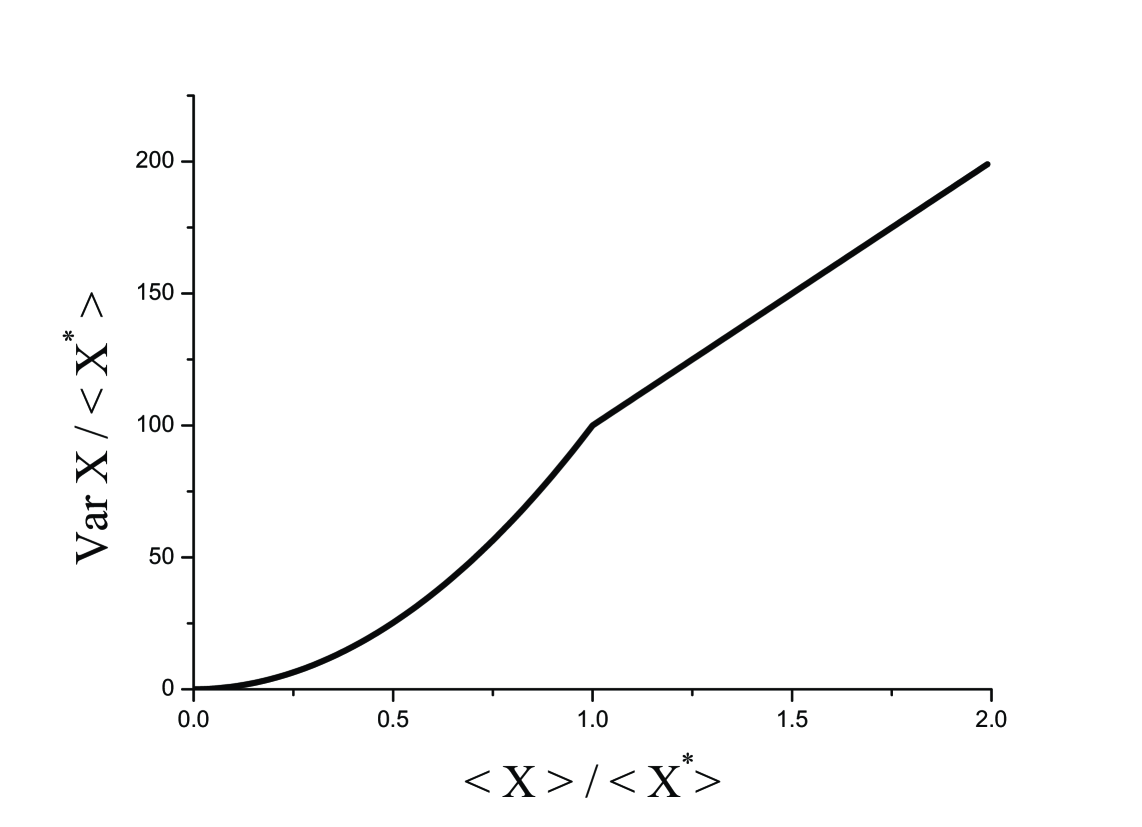
Figure 1: Dependence of the variance of infected individuals on the average for small populations which are part of a larger, well mixed population, $\langle X\rangle<\langle X^{*}\rangle$, or form an isolated population, $\langle X\rangle\geq\langle X^{*}\rangle$ (see eq.(17)). The infection rate is $\epsilon=0.01$.

For isolated patches, $b^{\prime}=0$ and $b/a=1-\epsilon$. As expected, the local and global values, eq.(13) and eq.(14) coincide, giving a ratio equal to $1/\epsilon$.

In a well mixed population, we have $b^{\prime}=b$, the total birth rate is $b_{\rm tot}=Mb$, and $(Mb)/a=1-\epsilon$. Then, we find:

$$\frac{{\rm Var}X_{i}}{\langle X_{i}\rangle} = 1+\frac{1-\epsilon}{M\epsilon}$$ (15)

$$\frac{{\rm Var}X}{\langle X\rangle} = \frac{1}{\epsilon}$$ (16)

For a small subsystem of a well mixed population ($M\gg 1/\epsilon$), we have ${\rm Var}X_{i}/\langle X_{i}\rangle\approx 1$. This ratio would imply that the process is due to random mutations with Poisson statistics. An analysis of the total variance, however, gives a rather different result. For large (but artificial) subdivisions of the well mixed system, $M\epsilon\ll 1$, and ${\rm Var}X_{i}/\langle X_{i}\rangle\approx 1/(M\epsilon)$.

It is interesting to analyze the situation in which populations of size $N$ below some size $N^{*}$ are part of a well mixed population of size $N^{*}$, while larger populations can be considered as isolated. made up of smaller, decoupled populations of size $N^{*}$. Then, for populations $N\leq N^{*}$ we can use eq.(15) with $M=N^{*}/N=\langle X\rangle/\langle X^{*}\rangle$ ($\langle X^{*}\rangle$ is the value of the mean of a population of size $N^{*}$), while when $N\geq N^{*}$ we can use eq.(16). The variance can be written as:

$${\rm Var}X=\left\{\begin{array}[]{lr}\langle X\rangle+\frac{\langle X\rangle^{2}(1-\epsilon)}{\langle X^{*}\rangle\epsilon}&N<N^{*}\\ \frac{\langle X\rangle}{\epsilon}&N\geq N^{*}\end{array}\right.$$ (17)

. Eq.(17) interpolates between a Poisson like regime for $N\ll N^{*}$ to a $1/\epsilon$ ratio between the variance and the mean for $N\geq N^{*}$. A sketch of the results is shown in Fig.[1]. used here imply that the coupling between different parts of the

5 Acknowledgements.

One of us (FG) is thankful to the Royal Society for a travel grant, and to the Royal Holloway for hospitality. F. G. also acknowledges financial support from grant MAT2002-0495-C02-01, MCyT (Spain). V. A. A. J. and N. S. acknowledge financial support from The Wellcome Trust Grant 063143. From eq.(4) one finds the equations:

$$\frac{d\langle Y_{i}\rangle}{dt} = (b-a)\langle Y_{i}\rangle+b^{\prime}\sum_{j\neq i}\langle Y_{j}\rangle+c$$

$$\frac{d\langle Y_{i}^{2}\rangle-\langle Y_{i}\rangle^{2}}{dt} = 2(b-a)\left(\langle Y_{i}^{2}\rangle-\langle Y_{i}\rangle^{2}\right)+(a+b)\langle Y_{i}\rangle+c+2b^{\prime}\sum_{j\neq i}\langle Y_{j}\rangle+b^{\prime}\sum_{i}\langle Y_{i}\rangle$$

$$\frac{d\langle Y_{i}Y_{j}\rangle-\langle Y_{i}\rangle\langle Y_{j}\rangle}{dt} = 2(b-a)\left(\langle Y_{i}Y_{j}\rangle-\langle Y_{i}\rangle\langle Y_{j}\rangle\right)+$$ (18)

$$+ b^{\prime}\sum_{i,j\neq k}\langle Y_{i}Y_{k}\rangle-\langle Y_{i}\rangle\langle Y_{k}\rangle+\langle Y_{j}Y_{k}\rangle-\langle Y_{j}\rangle\langle Y_{k}\rangle+$$

$$+ b^{\prime}\sum_{j\neq i}\langle Y_{i}^{2}\rangle-\langle Y_{i}\rangle^{2}+\langle Y_{j}^{2}\rangle-\langle Y_{j}\rangle^{2}$$

so that $\lim_{t\rightarrow\infty}\langle Y_{i}\rangle=Ke^{-[a-b-(M-1)b^{\prime}]t}+c/[a-b-(M-1)b^{\prime}]$ where $K$ is a constant determined by the initial conditions. We define:

$${C}_{ii} = \langle Y_{i}^{2}\rangle-\langle Y_{i}\rangle^{2}$$

$${C}_{ij} = \langle Y_{i}Y_{j}\rangle-\langle Y_{i}\rangle\langle Y_{j}\rangle$$ (19)

These quantities satisfy:

$$\frac{d}{dt}\left(\begin{array}[]{c}{C}_{ii}\\ {C}_{ij}\end{array}\right) = \left(\begin{array}[]{cc}2(b-a)&2(M-1)b^{\prime}\\ 2b^{\prime}&2(b-a)+(M-2)b^{\prime}\end{array}\right)\left(\begin{array}[]{c}{C}_{ii}\\ {C}_{ij}\end{array}\right)+$$ (26)

$$+ \left(\begin{array}[]{c}(a+b)\langle Y_{i}\rangle+b^{\prime}\sum_{j\neq i}\langle Y_{j}\rangle+c\\ 0\end{array}\right)$$ (29)

At long times, we find:

$$\lim_{t\rightarrow\infty}\left[(a+b)\langle Y_{i}\rangle(t)+b^{\prime}\sum_{j\neq i}\langle Y_{j}\rangle(t)+c\right]=\frac{2ac}{a-b-(M-1)b^{\prime}}$$ (30)

This leads to:

$$\lim_{t\rightarrow\infty}\left(\begin{array}[]{c}{C}_{ii}\\ {C}_{ij}\end{array}\right)=-\left(\begin{array}[]{cc}2(b-a)&2(M-1)b^{\prime}\\ 2b^{\prime}&2(b-a)+(M-2)b^{\prime}\end{array}\right)^{-1}\left(\begin{array}[]{c}\frac{2ac}{a-b-(M-1)b^{\prime}}\\ 0\end{array}\right)$$ (31)

References

• [1] N. Stollenwerk and V. A. A. Jansen, J. Theor. Biol. 222, 347-359 (2003).
• [2] N. Stollenwerk and V. A. A. Jansen, Phys. Lett. A 317, 87-96 (2003).
• [3] N. Stollenwerk, M. C. J. Maiden and V. A. A. Jansen, Proc. Natl. Acad. Sci. USA 101, 10229 (2004).
• [4] R. M. Anderson and R. M. May Infectious Diseases of Humans Oxford U. P., Oxford (1991).
• [5] V. A. A. Jansen, N. Stollenwerk, H. J. Jensen, M. E. Ramsay, W. J. Edmunds and C. J. Rhodes Science 301, 804 (2003).