Multicellular Tumor Spheroid in an off-lattice Voronoi/Delaunay cell model

Abstract

We study multicellular tumor spheroids by introducing a new three-dimensional agent-based Voronoi/Delaunay hybrid model. In this model, the cell shape varies from spherical in thin solution to convex polyhedral in dense tissues. The next neighbors of the cells are provided by a weighted Delaunay triangulation with in average linear computational complexity. The cellular interactions include direct elastic forces and cell-cell as well as cell-matrix adhesion. The spatiotemporal distribution of two nutrients – oxygen and glucose – is described by reaction-diffusion equations. Viable cells consume the nutrients, which are converted into biomass by increasing the cell size during $\rm G_{1}$-phase.

We test hypotheses on the functional dependence of the uptake rates and use the computer simulation to find suitable mechanisms for induction of necrosis. This is done by comparing the outcome with experimental growth curves, where the best fit leads to an unexpected ratio of oxygen and glucose uptake rates. The model relies on physical quantities and can easily be generalized towards tissues involving different cell types. In addition, it provides many features that can be directly compared with the experiment.

I Introduction

The spatiotemporal dynamics of individual cells often leads to the emergence of fascinating complex patterns in cellular tissues. For example, during embryogenesis it is hypothesized that these complex patterns develop with the aid of mechanisms such as diffusing messengers and cell-cell contact. Sometimes these patterns can be described very well with a simple model. Such mathematical models can help to test hypotheses in in silico experiments thereby circumventing real experiments which are very often expensive and time-consuming. However, since the local nature of cell-cell interactions is not precisely known one is often restricted to compare the global outcome following from different hypotheses with experimental data. Unfortunately, there are – unlike in theoretical physics – no established first principle theories in cell tissue modeling which explains that there is a variety of models on the market, which can be classified as follows:

Firstly, there is a class of models where one derives continuum equations for the cell populations. In analogy to many-particle physics one replaces the actual information on every cell by a cellular density. Consequently, the equations of motion can be simplified considerably to a differential equation describing the spatiotemporal dynamics of a cell type. In practice these equations do very often have the type of reaction-diffusion equations murray2002a . The volume-integral of such equations results in the global dynamics of a whole population (e.g. predator-prey-models), where only the temporal development of the total population is monitored. Note however, that cellular interactions can only be modeled effectively with these approaches. Also, the discrete and individual nature of cells is completely neglected.

The discrete nature can be taken into account by deriving master equations for the population number on every volume element shnerb2000 . By mapping these master equations to a Schrödinger equation one is able to identify an Hamilton operator that allows a physicist to apply the mathematical framework of quantum field theory to systems such as cell tissues. For example, in the simple case of Lotka-Volterra equations murray2002a this method leads to mean-field equations that resemble the Lotka-Volterra equations. The renormalized numerical results bettelheim2001 however may disagree qualitatively with the mean-field approximations. Consequently, the discrete nature of cells may not always be neglected. Still, the above quantization assumes all agents to be identical and indistinguishable and inevitably neglects the individuality of cells. Therefore, features such as cell shape and differences in cell size or internal properties are not considered in this class of models.

This is different in the third class of agent-based models, where cells are represented by individually interacting objects. Since now every single cell must be included in the computer simulations the computational intensity increases considerably. This however opens often the possibility to choose the interaction rules intuitively from existing observations. These models are usually restricted to a certain cell shape, which enables one to sub-classify them further: In lattice-based models deutsch1993 ; drasdo2002 the cellular shape is usually already defined by the shape of the elementary cell of the lattice, such as e.g. cubic meyerhermann2002 or hexagonal dormann2002 ; beyer2002 . Off-lattice models usually restrict to one special cell form and consider slight perturbations (e.g. deformable spheres drasdo1995 ; galle2005a or deformable ellipsoids palsson2000 ; palsson2001 ; dallon2004 ). In other off-lattice models the geometrical Voronoi tessellation honda2000 ; schaller2004 is used, which allows for more variations in cell shape and size. In addition, it comes very close to the polyhedral shape observed for some cell types honda1978 . An important advantage of off-lattice models is that perturbations from the inert cell shape can give rise to physically well-defined cellular interaction forces, whereas in lattice-based models one is usually forced to introduce effective interaction rules which makes it difficult to relate the model parameters to experimentally accessible quantities.

Since cell shape and function are usually closely connected (e. g. fibroblasts in the human skin do have a different shape than melanocytes or keratinocytes), there are some models that try to reproduce any possible cell shape. For example in the extended Potts model graner1992 ; savill2003 ; stott1999 ; turner2002 one has spins on several lattice nodes describing a single cell. The dynamics of these spins is calculated by minimizing an energy functional. The often-used Metropolis algorithm tests several spin flips for a decrease of the energy. A Metropolis time step is defined as having performed as many checks for spin flips as there are spins. The parameters in the energy functional have to be determined heuristically as it is difficult to map them to experimentally accessible microscopic properties. For example, volume conservation is usually handled by a penalty term which acts equally strong for both compression and elongation. The usual practice of relating the Monte-Carlo time step to physical time is not unique: There are cellular proliferation times, cellular compression relaxation times etc. Finally, the enormous number of spins required to appropriately describe a single cell leads to an enormous computational complexity that restricts the model to small cell numbers. This problem is circumvented in force-based models. For example in meyer_hermann2004 the relation of cell shape and cell motility has been investigated in a model that represents cells as a collection of cell fragments on a lattice. Other models describe cell shape on a 2-dimensional hypersurface by a changing number of polygonal nodes weliky1990 ; weliky1991 , which is also computationally expensive. In honda2004 , the initial configuration of the nodes bordering the polyhedral cells is deduced from a Voronoi tessellation of the cell centers, whereas the Voronoi concept is discarded during the dynamics, since every border node has its own dynamics. Generally, the latter models always need a large number of general coordinates to define the shape or status of a cell and are therefore restricted to a relatively small number of cells – even at present computational power.

Balancing these reasons in the context of the aimed description of in vitro tumor growth data we decided to use an off-lattice agent-based model, where one has the advantage of allowing continuous cell positions. Therefore the extent by which cellular interactions have to be replaced by effective automaton rules is much smaller than in corresponding cellular automata dormann2002 . In addition, the model parameters can be directly measured in independent experiments. The enormous computational intensity common to most existing off-lattice models is due to two effects: Firstly, some off-lattice models drasdo2002 use effective stochastic interaction rules, which require stochastic solution methods such as the Metropolis algorithm. The infinite number of possibilities in a continuous model however requires a large part of the phase space to be tested. Secondly, the determination of the neighborship topology for local interactions requires sophisticated algorithms. Our model uses the weighted Delaunay triangulation which provides the correct neighborship topology for a set of spheres with different radii with in average constant access schaller2004 . In addition, the model is dominantly deterministic which abolishes the necessity to test irrelevant parts of the phase space.

Unlike in two dimensions, where tumor cells in in vitro setups will proliferate without limitation, there exist growth limitations on tumor cell populations forming solid spheroidal cell aggregates in three dimensions folkman1973 . This limitation of growth is presumably due to both contact inhibition – which is also active in two dimensions galle2005a – and nutrient depletion in the interior of the spheroid. Initially, the cell number grows exponentially and enters a polynomial growth phase after some days in culture. Finally, a saturation of growth is observed for many spheroid systems freyer1986a . The final stages of spheroid growth exhibit a typical pattern in the cross-sections: An internal necrotic core is surrounded by a layer of quiescent cells – which do not proliferate – and on the outside one has a layer of proliferating cells mueller_klieser2002 . The final stage depends critically on the supply with nutrients such as oxygen and glucose. The model we have implemented enables us to model ${\mathcal{O}}\left(10^{5}\right)$ cells which is in agreement with cell numbers observed in multicellular tumor spheroid systems freyer1986a . We will demonstrate that the growth curves measured in freyer1986a for different nutrient concentrations can be reproduced using a single parameter set and simple assumptions for cellular interactions.

II The cell model

In our model we assume cells to be deformable spheres with dynamic radii, which is motivated by the experimental observation that cells in a solution tend to be spherical – presumably in order to minimize their surface energy. Consequently, we treat all deviations from this spherical form as perturbations from the inert cellular shape.

The model is agent-based (sometimes also called individual-based), i. e. every biological cell is represented by an individual object. These objects interact locally with their next neighbors (those that follow from the weighted Delaunay triangulation) and with a reaction-diffusion grid (for nutrients or growth signals). Each cell is characterized by several individual parameters such as position, a radius, the type corresponding to biological classifications, the status (position in the cell cycle), cellular tension, receptor and ligand concentrations on the cell membrane, an internal clock, and cell-type specific coupling constants for elastic and adhesive interactions. Since we assume the inert cell shape to be spherical, the power-weighted Delaunay triangulation schaller2004 is a perfect tool to determine the neighborship topology.

Figure 1: Two-dimensional illustration of inter-penetrating spheres with maximum overlap $h_{ij}$ and sphere contact surface $A_{ij}$ (marked bold). In reality, the spheres will deform and generate a repulsive force.	Figure 2: Within dense tissues, many-sphere-overlaps can occur. If in this case the Voronoi contact surface (marked with a bold line) is smaller than the sphere contact surface, it will provide a more realistic estimate of the cellular contact surfaces.

II.1 Elastic and adhesive Cell-Cell interactions

Following a model of Hertz hertz1882 ; landau1959 – which has already been used in the framework of cell tissues galle2005a ; wei2001 – the absolute value of the elastic force between two spheres with radii $R_{i}$ and $R_{j}$ can, for small deformations, be described as

$$F_{ij}^{\rm el}(t)=\frac{h_{ij}^{3/2}(t)}{\frac{3}{4}\left(\frac{1-\nu_{i}^{2}}{E_{i}}+\frac{1-\nu_{j}^{2}}{E_{j}}\right)\sqrt{\frac{1}{R_{i}(t)}+\frac{1}{R_{j}(t)}}}\,,$$ (1)

where $E_{i/j}$ and $\nu_{i/j}$ represent the elasticities and Poisson ratios of the spheres, respectively. The quantity $h_{ij}=\max\{0,R_{i}+R_{j}-\left|\mbox{\boldmath$r$}_{i}-\mbox{\boldmath$r$}_{j}\right|\}$ represents the maximum overlap the spheres would have if they would not deform but interpenetrate each other, see figure 2. In principle the repulsive force resulting from (1) could be overturned since it does not diverge for large overlaps. However, additional mechanisms (contact inhibition) insure that in practice the cells will respect a minimum distance from each other. In addition, the overlaps lead to a deviation of the actual cell volume (set intersection of Voronoi and sphere volume) from the intrinsic (target) cell volume. Therefore the cell volume is only approximately conserved within this approach.

In reality this model might not be adequate for cells: Firstly, the mechanics of the cytoskeleton is not well represented which might yield other than purely elastic responses (see e. g. alt1995 ; dallon2004 ). Secondly, equation (1) represents only a first order approximation which is valid for small virtual overlaps $h_{ij}\ll\min\{R_{i},R_{j}\}$ only. As cellular mechanics is known to be not only viscoelastic but also viscoplastic verdier2003 , a more exact approach would follow palsson2000 ; palsson2001 by replacing cells by equivalent networks containing elastic and viscous (internal cell friction) elements. However, the parameters required for such a model should either be measured for every cell type independently or they should be derived from a microscopic model of the cytoskeleton such as e.g. tensegrity structures ingber2003a ; ingber2003b , which is beyond the scope of this article. Consequently, internal cell friction is neglected. In addition, the Hertz model is only valid for two-body contacts, since for an exact treatment prestress and the difficult elastic problem of multiple overlaps will have to be considered as well. Therefore, especially in the case of multiple sphere overlaps (cf. figure 2) the Hertz model will underestimate the actual repulsion.

However, in this article we would like to restrict to the simple purely elastic model (1), since it allows the independently measurable experimental quantities $\nu_{i}$ and $E_{i}$ to be directly included.

Intercellular adhesion in a tissue is mediated by receptor and ligand molecules that are distributed on the cell membranes. For simplicity, we neglect a possible dynamical clustering of adhesion molecules and assume them to be – in average – uniformly distributed. The resulting average adhesive forces between two cells should then scale with their contact area $A_{ij}$ (see also e. g. palsson2000 ) and can be estimated as

$$F_{ij}^{\rm ad}=A_{ij}f^{\rm ad}\frac{1}{2}\left(c_{i}^{\rm rec}c_{j}^{\rm lig}+c_{i}^{\rm lig}c_{j}^{\rm rec}\right)\,,$$ (2)

where the receptor and ligand concentrations $c_{i}^{\rm rec/lig}$ are assumed to be normalized (i. e. $0\leq c_{i}^{\rm rec/lig}\leq c_{i}^{\rm rec/lig:max}\leq 1$) without loss of generality, since the – globally valid – coupling constant $f^{\rm ad}$ can always be rescaled by absorbing the maximum possible densities of receptors and ligands. Therefore the receptor and ligand concentrations do not have units but just represent the binding strength relative to a maximum binding absorbed in $f^{\rm ad}$ within this model. The contact surface area $A_{ij}$ can be estimated using the contact surface of two overlapping spheres $A_{ij}^{\rm sphere}$ – see figure 2.

Two issues need to be discussed in this respect: Firstly, the Hertz model predicts a contact surface of $A_{ij}^{\rm Hertz}=\pi(h_{i}+h_{j})R_{i}R_{j}/(R_{i}+R_{j})$, which is in the physiologic regime of parameters considerably smaller than the spherical contact surface $A_{ij}^{\rm sphere}=\pi(h_{i}R_{i}+h_{j}R_{j}-h_{i}^{2}/2-h_{j}^{2}/2)$. However, the spherical contact surfaces describe real tissue much more realistically than the Hertz contact surface, which should consequently rather be termed effective in the context of cellular interactions. In the used physiologic regime of overlaps the two contact surfaces have the same scaling in the first order. Therefore, a rescaling of the effective adhesive constant $f^{\rm ad}$ will replace the spherical contact surface by the Hertz contact surface. Secondly, in dense tissues the spherical contact surface is not a valid description anymore, since the contact surfaces of many spheres might overlap as in figure 2 inferring double-counting of surfaces and thus overestimating of the total cell surface.

The weighted Voronoi tessellation schaller2004 ; okabe2000 of a set of spheres $\{\mbox{\boldmath$r_{i}$},R_{i}\}$

$$V_{i}(t)=\{\mbox{\boldmath$x$}\in{\mathrm{R}}^{n}\; : \;\left[\mbox{\boldmath$x$}-\mbox{\boldmath$r_{i}$}(t)\right]^{2}-R_{i}^{2}(t)\leq\left[\mbox{\boldmath$x$}-\mbox{\boldmath$r_{j}$}(t)\right]^{2}-R_{j}^{2}(t)$$ (3)

$$\forall j\neq i\}$$

divides space into Voronoi regions – convex polyhedra that may in some sense be associated with the space occupied by cell $i$ (see figures 2 and 3). This correspondence however is deceptive, as one can easily show that equation (3) leads to infinitely large intercellular contact surfaces at the boundary of the convex hull of the points $\{\mbox{\boldmath$r_{i}$}\}$. In addition, in the case of a low cellular density the surfaces and volumes defined by the purely geometric approach (3) will evidently overshoot the actual cellular contact surfaces and volumes by orders of magnitude. On the other hand, Voronoi contact surfaces have been shown to approximate the cell shape in tissues remarkably well – at least in two-dimensional cross-sections honda1978 . Therefore, in order to have a contact surface estimate valid for different modeling environments we use a combination of the two approaches by setting

$$A_{ij}=\min\left\{A_{ij}^{\rm sphere}\,,A_{ij}^{\rm Voronoi}\right\}\,.$$ (4)

In order to use the Voronoi surface, cells do not only have to be in contact, but the Voronoi contact surface must be smaller than the spherical contact surface, which can be the case for multiple cell contacts, compare figure 2. This combination leads to upper bounds of intercellular contact surfaces on tissue boundaries and preserves the Voronoi surfaces within dense tissues by yielding a continuous transition between the two estimates. The underestimation of the repulsive forces in dense tissues within the Hertz model is in parts compensated by using the Voronoi-based decreased adhesive forces thereby leading to an increased net repulsion. Depending on the local cellular deformations the difference between the spherical and the Voronoi contact surface can be in the range of 30% within dense tissues.

Note that equations (1) and (2) allow for different cell types by introducing varying radii, elastic moduli and receptor and ligand concentrations.

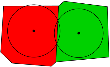
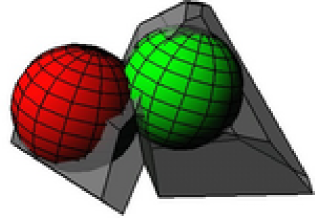
Figure 3: Visualization of two intersecting circles (spheres) and their corresponding Voronoi domains in two (three) dimensions. Position and orientation of the Voronoi contact line (plane) coincides with the circle (sphere) intersection. The Voronoi surfaces are also determined by the positions of other cells (not shown here).

All forces act in the direction of the normals to the next neighbors and on the center of the spheres. The total force on the cell $i$ is then determined by performing a sum over the next neighbors ${\mbox{\boldmath$F$}_{i}=\sum_{j\in{NN}(i)}\left(\mbox{\boldmath$F$}_{ij}^{\rm ad}-\mbox{\boldmath$F$}_{ij}^{\rm el}\right)\cdot\mbox{\boldmath$n$}_{ij}}$ and in addition we record the sum of the normal tensions

$$P_{i}=\sum_{j\in{NN}(i)}\frac{\left|\mbox{\boldmath$F$}_{ij}\cdot\mbox{\boldmath$n$}_{ij}\right|}{A_{ij}}\,,$$ (5)

where $\mbox{\boldmath$n$}_{ij}$ denotes the unit vector pointing from cell $i$ to cell $j$. The list of next neighbors is efficiently provided by the Delaunay triangulation. Once a force has been calculated, the corresponding spatial step can be computed from the equations of motion palsson2001 ; dallon2004

$$m_{i}\ddot{r}_{i}^{\alpha}(t)={F}_{i}^{\alpha}(t)-\sum_{\beta}\gamma_{i}^{\alpha\beta}\dot{r}_{i}^{\beta}(t)-\sum_{\beta}\sum_{j}\gamma_{ij}^{\alpha\beta}\left[\dot{r}_{i}^{\beta}(t)-\dot{r}_{j}^{\beta}(t)\right]\,,$$ (6)

where the upper Greek indices $\alpha,\beta\in\{0,1,2\}$ denote the coordinates and the lower Latin indices $i,j\in\{0,1,\ldots,N-1\}$ the index of the cell under consideration. The adhesive or repulsive forces as well as possible random forces on cell $i$ are contained in the term $F_{i}^{\alpha}$, whereas the coefficients $\gamma_{i}^{\alpha\beta}$ and $\gamma_{ij}^{\alpha\beta}$ represent cell-medium and cell-cell friction, respectively. A common isotropic choice for cell-medium friction is the normal Stokes relation

$$\gamma_{i}^{\alpha\beta,\rm visc}=6\pi\eta R_{i}\delta^{\alpha\beta}\,,$$ (7)

which describes the friction of a sphere with radius $R_{i}$ within a medium of viscosity $\eta$.

Most tissue simulations use the over-damped approximation $m_{i}{\ddot{r}}^{\alpha}_{i}(t)\approx 0\qquad\forall i,\alpha,t$, which is an adequate approximation for cell movement in medium howard2001 , since the estimated Reynolds-numbers are extremely small dallon2004 . Evidently, since additional adhesive bindings are at work, cellular movement in a tissue is even more damped drasdo2003a . In the over-damped approximation, equation (6) reduces to a $3N\times 3N$ linear system, that is sparsely populated and therefore can in principle be solved using an iterative method dallon2004 . However, the large number of cells involved in larger multicellular tumor spheroids would make this approach inefficient – both in terms of storage and execution time – and limits the simulations to ${\mathcal{O}}\left(10^{5}\right)$ cells. It is also not clear whether this intercellular drag force term significantly contributes. We have omitted this term and compensate for this by a modified friction model which respects that the movement of bound cells is considerably inhibited. In addition, one should keep in mind that within dense tissues many intercellular contacts are mediated by the extracellular matrix (with zero velocity). Such a friction term will rather contribute to the diagonal part of the dampening matrix. Therefore, we chose to approximate the term with the velocity differences by increasing the isotropic cell-medium friction coefficient by another term, i. e., $\gamma_{i}^{\alpha\beta}=\gamma_{i}^{\alpha\beta,\rm visc}+\gamma_{i}^{\alpha\beta,\rm ad}=\gamma_{i}\delta^{\alpha\beta}$ with

$$\gamma_{i}^{\alpha\beta,\rm ad} = \gamma^{\rm max}\delta^{\alpha\beta}\sum_{j\in{NN}(i)}A_{ij}\frac{1}{2}\left(1-\frac{\mbox{\boldmath$F$}_{i}\cdot\mbox{\boldmath$n$}_{ij}}{\left|\mbox{\boldmath$F$}_{i}\right|}\right)\times$$ (8)

$$\times\frac{1}{2}\left(c_{i}^{\rm rec}c_{j}^{\rm lig}+c_{i}^{\rm lig}c_{j}^{\rm rec}\right)\,,$$

as illustrated in figure 5. Note that the above ansatz for the friction coefficient scales with the intercellular contact surfaces and therefore cells having many bounds to next neighbors will move less than unbound cells. This is not an isotropic choice, since the forces contribute to its calculation. With using these approximations, the system (6) becomes diagonal, i. e.  one has

$$\mbox{\boldmath$\dot{r}$}_{i}=\frac{\mbox{\boldmath$F$}_{i}}{\gamma_{i}}\,.$$ (9)

As an option the model is capable of including random forces in order to mimic random cellular movement. However, the corresponding physiologic cellular diffusion coefficients are in the range of ${\mathcal{O}}\left(10^{-4}\rm\mu m^{2}/s\right)$, which leads to small displacements only. In the case of growing tumor spheroids, the proliferation-driven tumor front will generally overtake cells that have separated due to random movements. The stochastic nature contained in the mitotic direction and the duration of the cell cycle obviously suffices to yield isotropic tumor spheroids. The simulations shown here have therefore been performed without an additional stochastic force, unless otherwise noted.

II.2 The cell cycle

Figure 4: The extent to which adhesive bonds contribute to friction depends on the direction of movement and on the contact surfaces. If total force and normal vector are parallel, the corresponding contact surface will not contribute at all to the friction coefficient in equation (8), whereas the contribution will be strongest with force and normal vector being antiparallel.

Figure 5: During cell division, cells reside in the M-phase for $\tau^{(m)}$. Afterwards, the cell volume increases at a constant rate in the $\rm G_{1}$-phase, until the pre-mitotic radius $R^{\rm(m)}$ has been reached. At the end of the $\rm G_{1}$-phase, the cell can either continue the cell cycle or enter the $\rm G_{0}$-phase, if the normal tension $P_{i}$ exceeds a threshold. The ${\rm S}/{\rm G}_{2}$-phase lasts for a time $\tau^{\rm S/G_{2}}$, after which mitosis is deterministically initiated. The necrotic state can be entered at all times in the cell cycle.

In our model, cells have different internal states, which we chose to closely follow the cell cycle in order to make comparisons with experimental data as intuitive as possible. Consequently, the cellular status determines the actions of the cellular agents. We distinguish between 5 states: $\rm G_{1}$-phase, $\rm S/G_{2}$-phase, M-phase, $\rm G_{0}$-phase, and necrotic, see also figure 5.

During $\rm G_{1}$-phase, the cell volume grows at a constant rate $r_{\rm V}$, i. e. the radius increases according to $\dot{R}=\left(4\pi R^{2}\right)^{-1}r_{\rm V}$, until the cell reaches its final mitotic radius $R^{\rm(m)}$. The volume growth rate $r_{\rm V}$ is deduced by assuming that cell growth is only performed during during $\rm G_{1}$-phase

$$r_{\rm V}=\frac{2\pi\left(R^{\rm(m)}\right)^{3}}{3\tau_{\rm G_{1}}}\,,$$ (10)

where $\tau_{\rm G_{1}}$ can be deduced from the minimum observed cycle $\tau^{\rm min}$ time and the durations of the $\rm S/G_{2}$-phase and the M-phase. Afterwards, no further cell growth is performed. At the end of the $\rm G_{1}$-phase a checkpointing mechanism is performed where the cell can switch into $\rm G_{0}$-phase. If the cellular tension exceeds the threshold $P^{\rm crit}$ at this position in the cell cycle, the cell enters the $\rm G_{0}$-phase, otherwise the cell enters the $\rm S/G_{2}$-phase. Note that a different criterion for entering or leaving the $\rm G_{0}$-phase would also be possible: Cells might enter $G_{0}$-phase at any time in the cell cycle if the local nutrient concentrations fall below thresholds or – alternatively – if toxic substances exceed certain thresholds. In the present paper we will restrict to interpreting cellular quiescence as contact inhibition, since there is experimental evidence that in case of EMT6/Ro cells quiescence is not induced by lack of nutrients casciari1992 ; wehrle2000 .

During the S-phase the DNA for the new cell division is synthesized, whereas during $\rm G_{2}$-phase the quality of the produced DNA is controlled. In our model we do not distinguish between S-phase and $\rm G_{2}$-phase. At the beginning of the phase the individual phase duration is determined using a normally-distributed random number generator gammel2003 with a given mean and width. After this individual time has passed, the cells enter mitosis.

At the beginning of the mitotic phase – which lasts for about half an hour for most cell types – a mother cell divides and is replaced by two daughter cells. In the model these are slightly displaced in random direction, see subsection II.3. Afterwards the daughter cells are left to their initially dominating repulsive forces (1). As in the $\rm S/G_{2}$-phase the individual duration of the M-phase is determined using a normally-distributed random number generator. Afterwards the daughter cells enter the $\rm G_{1}$-phase thus closing the cell cycle. Note that we do not differentiate between the internal phases of mitosis.

During $\rm G_{0}$-phase, the cellular tension is monitored. Cells re-enter the cell cycle where they left it (i. e. at the beginning of the $\rm S/G_{2}$-phase) if the cellular tension falls below the critical threshold $P^{\rm crit}$. Similar to the $\rm S/G_{2}$-phase no growth is performed. Therefore in our model, the difference between the $\rm S/G_{2}$-phase and the $\rm G_{0}$-phase is that the duration of the first is determined by the normally distributed individual time, whereas for the duration of the latter the cellular tension is the determining factor. Consequently, the cells in $\rm G_{0}$-phase can serve as a reservoir of cells ready to start proliferating as soon as there is enough space available, which is common to many wound-healing models galle2005a .

Intuitively, cells enter necrosis as soon as the nutrient concentration at the cellular position falls below a critical threshold. We study different mechanisms for the induction of necrosis within the model and will be able to rule out possible candidates (see subsection III.1). Naturally, necrotic cells do not consume any nutrients and do slowly decay. In our model this is represented by removing these cells from the simulation at a rate $r^{\rm necr}$ – without performing prior shrinking.

Note that the only stochastic elements involved so far are the direction of mitosis and the durations of the M-phase and $\rm S/G_{2}$-phase. The first is required by the local assumption of isotropy, whereas the latter is required by the fact that proliferating cells having a common progenitor desynchronize rather quickly (usually after about 5 generations kreft1998 ): For these small systems of ${\mathcal{O}}\left(2^{5}\right)$ cells mechanisms such as nutrient depletion or contact inhibition cannot explain the desynchronization.

II.3 Proliferation

A cell will divide when the end of the $\rm S/G_{2}$ phase has been reached. The initial direction of mitosis is chosen randomly from a uniform distribution on the unit sphere gammel2003 , which is the simplest possible assumption. Note however that since the cellular movement during the M-phase is not only determined by the mitotic partners but also by the surrounding cells the effective direction of mitosis may generally change during M-phase – depending on the configuration of the next neighbors. The radii of the daughter cells are decreased $R^{\rm(d)}=R^{\rm(m)}2^{-1/3}$ to ensure conservation of the target volume during M-phase and the daughter cells are placed at the distance $d_{ij}^{0}=2R^{\rm(m)}(1-2^{-1/3})$ to ensure that initially the deformations of surrounding cells do not change drastically, see figure 6.

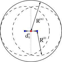
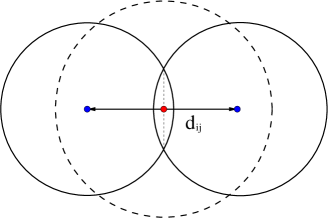
Figure 6: Illustration of the cell configuration right at proliferation (left) and at the end of the M-phase (right). At cell division, the radii of the daughter cells $R^{\rm(d)}$ are decreased to ensure conservation of the target volume during M-phase. The resulting strong repulsive forces drive the cells apart quickly. An adaptive timestep control ensures that the mitotic partners do not lose contact during M-phase.

One should be aware that at this stage the forces calculated in equation (1) cannot represent the actual mitotic separation forces, since the considerable overlap $h=R^{\rm(m)}(2^{5/3}-2)$ generates strong elastic forces in equation (1) which has then been applied far beyond its validity for small deformations. Therefore, to ensure for numerical stability, an adaptive step-size control has to be applied in the numerical solution of equation (6) – see the appendix – since otherwise the contact between the daughter cells might be lost immediately. Still, with an adaptive timestep, the initial separation of mitosis will happen on a timescale shorter than in reality. To the sake of simplicity we will not use modified mitotic forces within this article. One should keep in mind that the relative shortness of the M-phase in comparison with the complete cell cycle leads to a small fraction of cells being in the M-phase. Therefore, we expect the consequences of our simplifying assumption to be relatively small.

In figure 6 two cells are shown at proliferation and right after the M-phase. The bell-shape during mitosis resulting from the model is in qualitative agreement with the physiologic appearance of mitosis. One can also see that further intercellular contacts may be lost, if the neighboring cells reside perpendicularly to the direction of mitosis. The direction of mitosis will generally change during M-phase – and thus considerably differ from figure 6 right panel – and thereby the temporarily lost contact will in average be re-established, since the net forces will point to regions of low cell density and thus lead to closure of gaps. At the boundary of the spheroid however, cells may temporarily detach due to this mechanism. Though this had not been intended, it does not seem in contradiction to reality, since there exists experimental evidence landry1981 that EMT6/Ro tumor spheroids loose cells at the boundary due to mitotic loosening. A macroscopic detachment of cells from the spheroid boundary has not been observed in the simulation, since the spheroid growth velocity has always been large enough to re-establish contact after some time. However, such intermediate detachment events may very well contribute to the overall apparent growth velocity.

II.4 Nutrient consumption and Cell Death

We view cells as bio reactors where oxygen and glucose react to waste products as lactose, water and carbon dioxide. The clean combustion of glucose would require the molar nutrient uptake rate of oxygen to be 6 times the molar glucose uptake rate: $C_{6}H_{12}0_{6}+60_{2}\to 6H_{2}0+6C0_{2}$. However, for tumor tissue this cannot be the case as it is well-known that in the direct vicinity of tumors the concentration of lactic acid increases considerably which is a direct evidence for the incomplete combustion of glucose. By experimental estimations of average oxygen and glucose uptake rates for another cell line a considerable deviation from the ideal ratio has been found with about 1:1 kunz_schughart2000 . For EMT6/Ro cells, in wehrle2000 a ratio of about 1 : 3.9 is reported.

Thus, in our model all viable cells consume oxygen and glucose diffusing in the surrounding extracellular matrix at specific but constant rates.

The nutrient uptake rates can in principle depend on the cell type, the local concentration of both nutrients, the existence of internal cellular nutrient reservoirs and many other factors. However, few information about the qualitative dependence is known: most rates in the literature (see e. g. kunz_schughart2000 ) are average values given in units of mol per seconds and volume of tissue since these data are obtained from whole cell populations without regard to the individual cell size, status and the local nutrient concentration. In addition, the functional form of the dependence is unknown as well. The simplest starting point is to assume that the nutrient uptake rates only depend – if at all – on the local nutrient concentration. For example, when dealing with a single nutrient, quite often a Michaelis-Menten-like concentration-dependent nutrient uptake rate is assumed, see e. g. beuling2000 . This however means the introduction of further parameters that may be difficult to fix with the data available.

Depending on the cell type and on the local nutrient concentrations cells undergo apoptosis and/or necrosis when subject to nutrient depletion freyer1986a . In this specific application we choose necrosis as the dominant pathway to cell death and neglect the effects of apoptosis though there is experimental evidence that these processes are linked with each other bell2001 . Necrotic cells are randomly removed from the simulation with a rate $r^{\rm necr}$. The effect of apoptosis in the simulation would be similar, though apoptotic cells not break apart as necrotic cells but shrink and afterwards dissolve into small apoptotic bodies noble2003 . For the overall outcome of the total growth curve we expect insignificant changes by including apoptosis into the model.

With our computer simulation model we can test different hypotheses on which critical parameters may influence the onset of necrosis: For example, there could be two critical concentrations for both oxygen and glucose or just one combined parameter with an unknown dependence on the local concentrations. In addition, there could also be other processes such as necrotic waste material inducing apoptosis and/or necrosis, which will not be considered here.

II.5 Nutrient distribution

We consider the case of avascular tumor growth and therefore assume that the transport of nutrients is performed passively by diffusion. Consequently, the diffusion through tumor tissue and also through the culture medium is described by a system of reaction-diffusion equations

$$\frac{\partial u^{\rm ox/gluc}}{\partial t} = \vec{\nabla}\left[D^{\rm ox/gluc}(\mbox{\boldmath$x$};t)\vec{\nabla}u^{\rm ox/gluc}(\mbox{\boldmath$x$},t)\right]$$ (11)

$$-r^{\rm ox/gluc}(\mbox{\boldmath$x$};t)\,,$$

where $u^{\rm ox/gluc}(\mbox{\boldmath$x$},t)$ describes the local oxygen or glucose concentration, $D^{\rm ox/gluc}(\mbox{\boldmath$x$};t)$ the local effective oxygen or glucose diffusion coefficient (which depends implicitly on time via the cellular positions) and $r^{\rm ox/gluc}(\mbox{\boldmath$x$};t)$ the local oxygen or glucose consumption rate. Though formally equation (11) might admit negative nutrient concentrations (even at low concentrations strong negative sink terms may in principle exist), this can never happen in reality – provided the timestep is not too large: Cells will enter necrosis (thereby stopping nutrient consumption) if the local nutrient concentrations become too small. As the reaction rates depend on the cellular status, they become implicitly dependent on the nutrient concentrations, see also subsections II.2 and II.4.

In equation (11) we implicitly assume that the transport of matter can be described by an effective diffusion coefficient. This does not have to be the case, since cellular membranes pose complicated boundary conditions especially for larger molecules such as glucose. In addition, convection may also contribute to matter transport. Only if the tissue is isotropic on scales larger than a cell diameter this assumption is justified. Consequently, the discretization of equation (11) does only make sense on lattices with spacings exceeding the cellular diameters.

Though we use an effective diffusion coefficient $D_{\rm eff}$ it is sometimes necessary to allow for diffusivities varying on scales larger than the cell diameter – especially for larger molecules. For example, the effective diffusion coefficient of glucose is about 700 $\rm\mu m^{2}/s$ in water, whereas it is only 100 $\rm\mu m^{2}/s$ in tissue casciari1988 . This effect is less pronounced for smaller molecules such as oxygen with about 2400 $\rm\mu m^{2}/s$ in water and 1750 $\rm\mu m^{2}/s$ in tissue grote1977 . Consequently, when modeling in vitro multicellular tumor spheroids one will have to take spatially varying diffusivities into account to appropriately model the nutrient concentrations on the spheroid boundary. In our model, the diffusion constant is set to measured tissue diffusivities in the vicinity of cells and to the normal diffusivities in water anywhere else. Therefore, by considering varying diffusivities one is able to keep the rectangular shape of the diffusion grid which is favorable for the numerical solution, see also the appendix. Note that a diffusion-depletion zone as in groebe1996 is thereby automatically incorporated into the model. The difference is that here the model does not a priori impose spherical symmetry. It can be checked however by direct observation of the spherically-shaped nutrient isosurfaces, that the rectangular shape of the boundary does not greatly influence the nutrient distribution near the tumor.

Another possibility would be to solve the nutrient diffusion within the spheroid only by assuming a spherical tumor symmetry with a time-dependent boundary moving with the spheroid size. However, with such an approach the spherical symmetry would not be an outcome but an intrinsic ingredient of the model. Consequently, in such a model the spheroid shape would not be of any comparative value.

Equation (11) does only have a defined solution if the initial conditions and the boundary conditions are set. As in freyer1986a it has been verified that the nutrient concentration outside the tumor spheroid did not vary strongly between the periodic refilling of nutrients, we approximated the experimental system by imposing Dirichlet boundary conditions throughout the simulation. The corresponding initial and boundary concentrations have both been set to the values used in the experiment.

III Results

III.1 Population Dynamics

The overall cell number is a parameter which can be quantified experimentally, either indirectly by simply calculating cell numbers from observed tissue volumes or directly by extensive automated cell-counting. In freyer1986a the cell number has been determined indirectly for different concentrations of oxygen and glucose. With our model we have calculated growth curves for different nutrient concentrations and different hypotheses of nutrient uptake and necrosis induction. The simulations have been compared with four series of experimental data, where four different combinations of oxygen and glucose concentrations have been investigated. Naturally, within one set of simulations all parameters but the nutrient concentrations have been kept fixed.

We have tested the possibility that there exist critical concentrations for the two nutrients separately. However, in this case either the glucose or oxygen concentration dominantly limit the cell population dynamics. This does not reproduce the experimental data freyer1986a , since the growth curves for one of the nutrient concentrations being kept constant depend strongly on the concentration of the other nutrient. Therefore, since low oxygen and large glucose concentrations can result in similar population dynamics as large oxygen and low glucose concentrations (freyer1986a ), both concentrations must enter the critical parameter. We have also tested the possibility of concentration-dependent nutrient consumption rates with the functional form of the Michaelis-Menten type kinetics

$$r^{\rm nut}=r^{\rm min}+\frac{(r^{\rm max}-r^{\rm min})C^{\rm nut}}{C_{1/2}+C^{\rm nut}}\,.$$ (12)

This model however uses additional parameters that cannot be fixed with the present data – even when omitting $r^{\rm min}$. In addition, the values for $C_{1/2}$ in the literature for oxygen-dependent proliferation roose2003 of $0.0083$ mM point into the direction that the oxygen consumption rates are always within the range of saturation, since the local oxygen concentration has always been larger than 0.04 mM throughout the spheroids. Consequently, we have assumed constant cellular oxygen and glucose uptake rates for non-necrotic cells in the present model. We chose the product of oxygen and glucose concentration to be the limiting factor to sustain cellular viability. This simple ansatz did suffice to reproduce the experimental cellular growth curves (see figure 7). The best fit is achieved with the parameter set shown in table 1. The corresponding tumor morphology is addressed in subsection III.2.

Unfortunately, no error bars are given in freyer1986a and the experimental data scatter considerably even on a logarithmic scale, see figure 7. Apart from the difficulty of establishing a defined experimental system in biology, this large scatter is also due to the necessity of destroying the spheroids during the measurements. Therefore, a whole ensemble of spheroids had to be measured. Since the monoclonality of these spheroids is not ensured, it is not a priori clear whether a single spheroid might contain several species or whether different spheroids might belong to different species with individual growth characteristics. In order to employ a procedure to minimize deviations between the simulation and experimental data we defined estimated error bars by calculating the difference to the artificial Gompertz growth curve

$$N(t)=N_{0}\exp\left[\frac{\alpha}{\beta}\left(1-e^{-\beta t}\right)\right]\,,$$ (13)

which is known to reproduce most growth processes in nature with remarkable accuracy ling1993 .

Not every hypothesis on nutrient consumption and necrosis induction leads to acceptable agreement with experimental data – indicating the sensitivity of the model. The theoretical predictions lie within the scattering region, see figure 7.

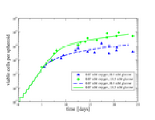
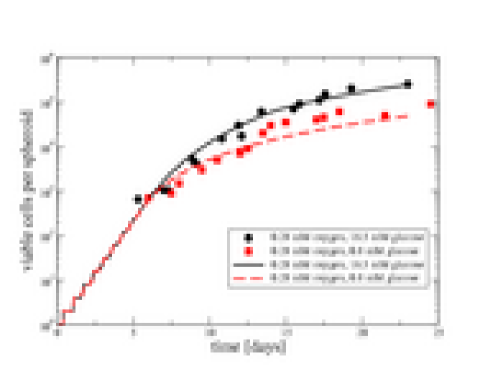
Figure 7: Number of viable cells per spheroid for 0.8 and 16.5 mM glucose concentrations and either 0.07 mM oxygen concentration (left panel) or 0.28 mM oxygen concentration (right panel). Experimental data (symbols) were read off from freyer1986a , whereas lines correspond to the computer simulations.

Qualitatively, one can see that for all the simulations the initial exponential growth phase soon enters a crossover to a polynomial growth. In our model this crossover is due to two distinct mechanisms – contact inhibition and nutrient depletion – which lead to the similar outcome that after a certain time dominantly the spheroid surface will contribute to the proliferation, i. e.

$$\frac{dN}{dt}=\alpha N^{2/3}\,,$$ (14)

which has the polynomial solution $N(t)=N_{0}\left[1+\beta t+\beta^{2}t^{2}/3+\beta^{3}t^{3}/27\right]$ with $\beta=\alpha/N_{0}^{1/3}$ mueller_klieser2002 . Apart from the fact that necrosis is evidently more likely when nutrients are rare, the mechanisms cannot be clearly distinguished with a glance at the total growth curves in figure 7. Even in the case where both nutrients are rare, the growth curve can be fitted by above equation: The scatter of the data does not allow to exclude this possibility. However, given that tumor spheroids saturate at a certain size, the above model cannot be valid in all regimes of tumor growth.

Since the mechanism of contact inhibition leads to cells resting in $\rm G_{0}$ rather than cells entering necrosis the differences can easily be analyzed in the cell cycle distribution. In figure 8 it is evident that for 0.07 mM oxygen and 0.8 mM glucose concentrations (upper left panel) the nutrient starvation is the dominant limiting factor to cell cycle inhibition, since there are nearly no cells in $\rm G_{0}$-phase and the majority of cells is necrotic. In the case of nutrient abundance (0.28 mM oxygen and 16.5 mM glucose, figure 8 lower right panel) however, the majority of cells resides in $\rm G_{0}$-phase during days 6-23, which is an indication for contact inhibition being the dominant reason for the crossover, as is also assumed in other models galle2005a ; drasdo2003a . This is also confirmed by the cross-sections of the computer simulated tumor spheroids, see figure 9. Though in the case of nutrient abundance necrosis sets in much later, the number of necrotic cells rises at a much stronger slope and it is to be expected that necrosis will displace the contact inhibition as the major cause for surface-dominated growth after 25 days (with overall roughly $5\times 10^{5}$ cells involved, the simulations become very extensive and memory-consuming). Such a displacement of dominating mechanisms is already visible for some intermediate nutrient concentrations. For example, in the case of $0.07$ mM oxygen and $16.5$ mM glucose concentrations the number of cells in $\rm G_{0}$-phase first rises to reach its maximum after 10 days and afterwards decays in combination with a strong rise in necrotic cells (figure 8, upper right panel). Such a behavior is not observed in the regime of large oxygen and low glucose concentrations (figure 8 lower left panel), where necrosis and contact inhibition set in simultaneously and nutrient starvation is the main limiting factor. This is due to the considerably decreased glucose diffusion coefficient in tumor tissue, whereas the diffusion coefficient of oxygen is nearly the same in tissue and water, compare subsection II.5. Consequently, the already low glucose concentration of 0.8 mM at the boundary drops rapidly when the number of tumor cells increases, since new glucose supply diffuses very slow from the outside.

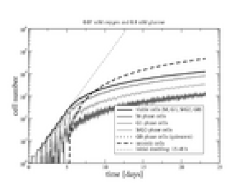
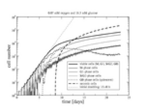
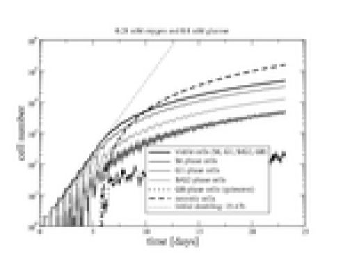
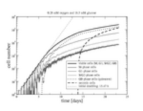
Figure 8: Cell cycle distribution for different oxygen and glucose concentrations. Depending on the external nutrient concentrations, significant differences mark the dominance of different mechanisms to limit the cell cycle. Fits to the regions of exponential growth – marked by the complete absence of necrotic and quiescent cells – reproduce the shortest observed cycle time within statistical fluctuations. The initial oscillations in the sub-populations in the cell cycle stem from the fact that the cells divide synchronously at the beginning – their frequency is the inverse cell cycle time. After each cell division, the daughter cells draw new duration times for the $\rm S/G_{2}$-phase and the $M$-phase from a Gaussian distribution, compare table 1, which leads to a dampening of the oscillations and finally to complete desynchronization of cell division. The occurrence of contact inhibition or necrosis increases the dampening effect, since the migration through the cell cycle is impaired. Note that in the case of few nutrients contact inhibition does not play a role, as there are no quiescent cells (top left).

III.2 Tumor Spheroid Morphology

To estimate the quality of a mathematical model one has to find experimentally accessible parameters. This is especially difficult when thinking about tissue morphology, since very often the patterns are hard to quantify in terms of numbers. The morphology of three-dimensional tumor spheroids is rather simple: An inner necrotic core is surrounded by a layer of quiescent cells, which is in turn surrounded by the outer layer of proliferating cells. Qualitatively, this morphology is well reproduced in the case of initial nutrient abundance, see upper right panel in figure 9. In the case of nutrient starvation however there is virtually no layer of quiescent cells (figure 9 upper left panel), as contact inhibition is not of importance in this scenario (see figure 8 upper left panel). This would be different if quiescence is induced by nutrient limitations: In this case, the necrotic core would always be surrounded by a layer of quiescent cells. Indeed, experimental observations casciari1992 suggest that neither nutrient depletion nor the related acidic pH induce the cellular quiescence. It is evident from figure 9 that the size of the layers depends on the boundary concentrations. In addition, it also depends on the nutrient consumption rates and diffusivities of oxygen and glucose within the tumor tissue. The size of the necrotic core is also very sensitive on the rate at which necrotic cells are being removed from the simulation.

Note that in the spheroid cross-sections it is evident that – if oxygen and/or glucose are limited – a relatively small number of cells with constant nutrient uptake rates suffices to drop the nutrient levels under the critical threshold thus leading to the onset of necrosis and the absence of a layer of quiescent cells in the end of the simulations, compare also figure 8. This is different for a model with concentration or cell-cycle dependent nutrient uptake rates. In the first case the absolute value of the nutrient concentration gradients would be decreased thus giving rise to a broader viable layer which – in turn – could allow for the existence of a quiescent layer. In the second case the intermediate emergence of cellular quiescence (see figure 8) would also decrease the absolute value of the nutrient concentration gradient towards the necrotic core, which would prolong and eventually stabilize the existence of a quiescent layer also for nutrient depleted configurations. Therefore, in order to distinguish between nutrient uptake models, the tumor spheroid morphology is an important criterion, whereas the simple total growth curve is not sufficient to make quantitative predictions about the mechanisms at work.

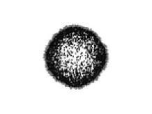
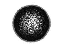
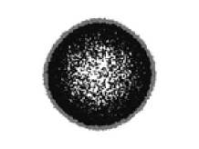
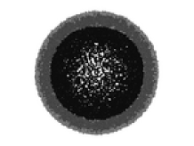
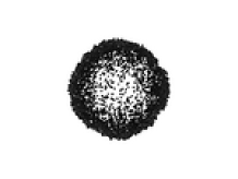
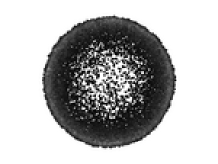
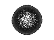
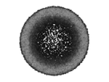
Figure 9: Cross-section of computer-simulated tumor spheroids after $23$ days of simulation time. The first row shows the cellular status (necrotic cells painted black, quiescent cells in dark grey, cells in the cell cycle in lighter shades of grey), whereas the second row visualizes the cellular tension (free cells painted black, cells under strong pressure in light grey). Nutrient concentrations from left to right are given by $0.07$ mM oxygen and $0.8$ mM glucose, $0.07$ mM oxygen and $16.5$ mM glucose, $0.28$ mM oxygen and $0.8$ mM glucose, and $0.28$ mM oxygen and $16.5$ mM glucose.

Interestingly, the spheroids in figure 9 are fairly round, especially for the case where nutrients are provided in abundance. This is due to the stochastic nature of the mitotic direction which forces initial differences to average out after some time – which can easily be verified by restarting the computer code with similar parameters but different seed values for the random number generator (data not shown). This is in agreement with many spheroids observed in the experiment freyer1986a and in other computer simulations drasdo2003a . However, the spheroids are less spherical for extreme nutrient depletion, since firstly the small cell number yields less stochastic events that contribute to the averaging and secondly the emergence of localized holes in the necrotic core is not counterbalanced by a strong mainly isotropic proliferative pressure from the proliferating rim – as is the case for large nutrient concentrations. The sometimes observed deviations from the spherical form freyer1986a can also have additional reasons: The spheroids might be hetero-clonal while all cells in our simulation are assumed to be monoclonal. If a spheroid does not develop from a single but two genetically differing cells, these cells might exhibit different growth characteristics.

III.3 Parameter Dependence

The growth curves shown in figure 7 have been calculated using the – comparably many – parameters in table 1.

parameter	value	unit	comment
ECM viscosity $\eta^{\rm VISC}$	$5\cdot 10^{-3}$	$\rm kg/(\mu ms)$	galle2005a , estimate
adhesive friction $\gamma^{\rm max}$	0.1	$\rm kg/(\mu m^{2}s)$	galle2005a , estimate
receptor concentration $c^{\rm rec}$	1.0	#	fixed
ligand concentration $c^{\rm lig}$	1.0	#	fixed
oxygen diffusivity $D_{\rm eff,ox}^{\rm tissue}$	1750.0	$\rm\mu m^{2}/s$	grote1977
glucose diffusivity $D_{\rm eff,gluc}^{\rm tissue}$	105.0	$\rm\mu m^{2}/s$	casciari1988
mitotic phase $\tau^{\rm(m)}$	$(3.6\pm 0.9)\cdot 10^{3}$	s	estimate
$\rm S/G_{2}$-phase $\tau^{\rm S/G_{2}}$	$(18.0\pm 7.2)\cdot 10^{3}$	s	estimate
shortest cycle time $\tau^{\rm min}$	$54.0\cdot 10^{3}$	s	landry1981 ; freyer1986a ; casciari1992 , estimate
mitotic cell radius $R^{\rm(m)}$	$5.0$	$\rm\mu m$	estimate
cell elastic modulus $E$	$1.0\cdot 10^{-3}$	MPa	galle2005a , estimate
cell Poisson number $\nu$	$0.5$	#	assumption
adhesive coefficient $f^{\rm ad}$	$1.0\cdot 10^{-4}$	$\rm\mu N/\mu m^{2}$	eq. overlap
necrosis absorption rates $r^{\rm necr}$	$2.0\cdot 10^{-6}$	cells/s	estimate/fit
critical cell tension $P^{\rm crit}$	$0.6\cdot 10^{-3}$	MPa	fit parameter
oxygen uptake $r^{\rm ox}$	$20.0\cdot 10^{-18}$	mol/(cell s)	fit parameter
glucose uptake $r^{\rm gluc}$	$95.0\cdot 10^{-18}$	mol/(cell s)	fit parameter
critical product $p^{\rm oxgluc}$	$0.025$	$\rm mM^{2}$	fit parameter

Table 1: Best fit model parameters that are used in the simulations shown in figures 7, 8, and 9. See text for explanations.

However, since mainly deterministic and rather physically-motivated interactions are assumed, more parameters than in PDE or cellular automaton models can be accessed by independent experiments and do not need to be varied as fit parameters. Some of these parameters deserve special attention: The elastic parameters of EMT6/Ro tumor cells might differ from those in our simulation, where incompressibility has been assumed – see table 1. Assuming reduced Poisson ratios $\nu\approx 0.3$ and elasticities of $E\approx 750$ Pa galle2005a ; roose2003 , one may obtain deviations in the elastic forces in (1) in the range of up to 50 percent. However, even with these different elastic constants the growth characteristics does not change significantly: This is due to the fact that the cellular tensions relax on a much shorter timescale than the cell cycle time. An initial cycle time of 17 h has been obtained in freyer1986a using a Gompertz fit to the spheroid volume. This fit had been applied to already existing small spheroids that may exhibit growth retardation effects. For cells that had separated at the spheroid boundary, a cell cycle time of only 13 h landry1981 has been observed. Therefore – and in order to reproduce the slopes correctly – we have used a slightly decreased shortest possible cycle time. The cell tension defined here is simply a sum over all normal tensions with the next neighbors. The value that we have obtained as fit parameter is about 6 times as large as the critical cellular compression used as a criterion for contact inhibition in similar simulations (90 Pa in galle2005a ). In part, this may be due to the Voronoi surface correction – surfaces tend to be smaller than sphere surfaces – which leads to generally larger normal tensions. The remaining discrepancy should be attributed to the fact that we use a different cell line and the inherent model differences. The removal rate $r$ of necrotic cells did not have a considerable impact on the macroscopic number of viable cells and the spheroid size. However, it can also be seen in figure 9 that due to the removal of necrotic cells holes emerge. Then the mechanical coupling from the necrotic tumor core towards the boundary will be disrupted. Therefore, for the used elastic and adhesive parameters, the parameter $r$ mainly controls the number of necrotic holes in the center. Note that this is different however, in a scenario with considerably increased adhesion, where the mechanical coupling is not disrupted and the rate constant $r$ does have an influence on the spheroid size and thereby on the overall cell number.

In accordance with the assumption of contact inhibition being the dominant cause for the crossover from exponential to polynomial growth in the case of nutrient abundance, the initial phases of the theoretical growth curve for $0.28$ mM oxygen and $16.5$ mM are dominantly dependent on the critical cell tension, whereas the other growth curves – especially for nutrient depletion – strongly depend on the nutrient uptake rates and the necrotic parameter. Generally, the late stages of spheroid growth depend critically on the nutrient-related parameters. The resulting parameters for nutrient uptake rates are well within the range observed in the literature casciari1992 ; wehrle2000 ; groebe1991 ; freyer1985 ; freyer1986a , though some considerable variances even within the literature exist. Apart from the fact that mostly different cell lines are analyzed, the additional problem exists that the values in the literature are usually volume-related uptake rates that have been fitted on experimental data. Consequently, the extracted cellular uptake rates depend on the corresponding cellular packing density of these systems. It must be kept in mind that these rates represent average values over the whole ensemble of cells present in the spheroid. For example, quiescent cells could have a considerably-decreased nutrient uptake rate. In addition, there is evidence that glucose uptake rates can be related to the local concentration of available oxygen casciari1992 . The present quality of the data however does not allow to discriminate between more sophisticated models

Note that in the over-damped approximation of equation (6) the solution is calculated as a ratio of combined elastic and adhesive forces to a friction parameter, which is largely influenced by cell-cell adhesion. Therefore, the model will not be very sensitive on the specific adhesion coupling constants and the adhesion-determined friction, as rather their ratio is mainly influencing the model behavior as long as elastic forces are small.

III.4 Saturation of growth curves

A complete saturation of the cell number or spheroid size – as suspected by freyer1986a and others folkman1973 – cannot be reproduced in the computer simulations with the parameters in table 1. The large scatter of the data in the case of nutrient depletion (figure 7 left panel) does not exhibit a clear saturation within 25 days, which is not reached in the other configurations anyway. For the explanation of a growth saturation the nature of the additional mechanism remains controversial. For example, in folkman1973 an effective movement of cells towards the necrotic core has been observed leading to the assumption of a chemotactic signal secreted by necrotic cells. The corresponding computer simulations in dormann2002 did lead to saturation. Since it is somewhat arbitrary to assume that tumor cells follow a necrotic signal we also tested a simpler hypothesis:

In figure 9 macroscopic holes are visible within the necrotic core – created by the removal of necrotic cells from the simulation. Once such a hole is established, it even tends to grow, since the intercellular adhesion is of very short range. (Recall that equation (2) depends on the contact surface.) We have found that an increase of adhesive normal forces to $f^{\rm ad}=$ 0.0003 $\rm\mu N/\mu m^{2}$ suffices to close the visible holes completely – thereby inevitably coupling the proliferating ring to the necrotic core which finally leads to apparent growth saturation, compare figure 10. Note however, that in the presence of stochastic forces, complete saturation (lasting infinitely long) can never be observed, since already the seldom case of cells leaving the spheroid will lead to further colonies that might recombine. Consequently, the volume loss generated by removing necrotic cells with a certain rate must be balanced by a movement of proliferating or quiescent cells from the outer layers into the necrotic core. In addition, the outward component of the proliferative pressure on the outer layer is counterbalanced by the increased cellular adhesion as well. For such a system, a growth saturation is inevitable: As in the late stages of spheroid growth the cellular birth rate can be assumed to be proportional to the spheroid surface $R_{\rm birth}\approx\alpha N^{2/3}$ and the rate of cell removal is proportional to the number of necrotic cells residing in the center, the total cell number can be described by

$$\frac{dN}{dt}=\alpha N^{2/3}(t)-\beta\left[N(t)-\gamma N^{2/3}(t)\right]$$ (15)

with $\alpha,\beta,\gamma$ being positive constants. Above equation resembles the growth law of Bertalanffy ling1993 . The solution of this equation reaches the steady state $N_{\infty}=\left(\frac{\alpha}{\beta}+\gamma\right)^{3}$, which is stable for $\beta>0$. Therefore, in this regime the nutrient depletion is the dominant factor limiting tumor spheroid growth.

We conclude that growth saturation of both cell number and spheroid radius in off-lattice computer simulations can be reached by assuming increased intercellular adhesion forces. In that case viable cells move towards the necrotic core (data not shown). The assumption of some diffusing signal as in dormann2002 is not necessary. Interestingly, during the period of saturation, deviations from the spherical shape can emerge: The position of unstable intermediate holes within the necrotic core is randomly distributed and gives rise to macroscopic deviations from spherical shape on the spheroid surface. Therefore, an irregular spheroid shape can also be explained by individual durations of the necrotic process. Note that another candidate for a cell loss mechanism is shedding of cells at the spheroid surface landry1981 ; landry1982 . All these mechanisms might could be combined with an involvement of metabolic waste products in the induction of necrosis.

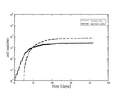
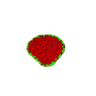
Figure 10: After assuming an increased adhesive coupling the emergence of holes within the necrotic core is completely inhibited. In addition, the cells have been displaced randomly by a Gaussian distribution with width $\Delta x_{i}=\sqrt{2D\Delta t}$ at every timestep. A steady-state flow equilibrium is established leading to approximate growth saturation of the spheroid (left) in the observed time range. No further mechanisms need to be assumed. In addition, the fast closure of holes in the necrotic core can lead to deviations from the spherical symmetry (right). Cells in the cell cycle are marked in light grey, quiescent cells in grey and necrotic cells are depicted by dark grey.

IV Summary

We have demonstrated that the Voronoi/Delaunay hybrid model can very well be used to establish agent-based cell-tissue simulations. The Voronoi/Delaunay approach provides some advantages: Firstly, compared to the description of cells by deformable spheres, the Voronoi tessellation provides an improved estimate of contact surfaces within dense tissues. The present model combines the advantages of both model concepts. Secondly, the weighted Delaunay triangulation is an efficient method to determine neighborship topologies for differently-sized sphere-like objects. In addition, it can efficiently be updated in the case of moving objects. The model is very rich in features and therefore allows many comparisons with the experiments. It can easily be combined with established models on cellular adhesion and elasticity that rely on direct experimental observables. Therefore it allows some of its parameters to be fixed by independent experiments. The parameters which had to be determined with respect to macroscopic quantities represent existing physical quantities. Since such quantities can be falsified in future experiments, the model provides predictive power to a greater extent than differential equation or cellular automaton approaches.

Unlike previous models dormann2002 ; drasdo2003a ; groebe1996 – which only considered the influence of one nutrient on the dynamics of three-dimensional multicellular tumor spheroids – we were able to reproduce the experimental growth curves with a single parameter set by considering the spatiotemporal dynamics of both the oxygen and glucose concentrations simultaneously. A saturation of growth could be obtained by increasing intercellular adhesive forces threefold.

On the one hand, the typical spheroid morphology is reproduced qualitatively very well. On the other hand, a quantitative reproduction not only of cell population growth curves but also of spheroid morphology could allow for a more detailed analysis of nutrient consumption models: For a different cell line an oxygen : glucose uptake ratio of about 1:1 has been found kunz_schughart2000 . In contrast, our computer simulations point to the scenario that the oxygen consumption rates are much smaller (about 1:5) than the glucose consumption rates (table 1), though the values are within the ranges of uptake rates in the literature if considered separately. This discrepancy may be due to several reasons. Firstly, there is strong experimental evidence that the ratio of oxygen and glucose uptake in the case of EMT6/Ro cells considerably differs even from the ratio of 1 : 1. For example, in wehrle2000 a ratio of 1 : 3.9 is suggested. Secondly, the effective diffusivities within tissue for oxygen and glucose obtained from grote1977 and casciari1988 might not be correct – this would lead to different currents of oxygen and glucose within the spheroid. Thirdly, the model assumptions of roughly constant nutrient uptake rates and the product of both concentrations being the critical parameter for necrosis might not be correct.

We have seen that the quantitative analysis of the overall growth curve can in principle be used to determine unknown parameters. The current experimental data however exhibit too much scatter to determine parameters with accuracy, therefore a combined experimental and theoretical investigation of multicellular tumor spheroids of a single well-defined cell line is of urgent interest.

The presented model is especially suitable for systems with a comparably large number of cells. In addition, it supports different cell types as well. The cell shape however, is restricted to convex cells. This makes it suitable to model rather dense cell tissues such as e. g. epithelia where one can investigate the roles of differential adhesion, elastic interactions and active cellular migration in tissue flow equilibrium. Further applications of the Voronoi/Delaunay method will therefore include the modeling of epithelia, bone formation, and bio films. In addition, the weighted Delaunay triangulation is a suitable tool for the modeling of boundary conditions e. g. in froths.

V Acknowledgments

G. Schaller is indebted to T. Beyer and W. Lorenz for discussing many aspects of the algorithms and testing the code. J. Galle is being thanked for his advice on cellular interactions. G. Schaller was supported by the SMWK. M. Meyer-Hermann was supported by a Marie Curie Intra-European Fellowship within the Sixth EU Framework Program.

VI Appendix

VI.1 Program Architecture

The programming language $C++$ supports object-oriented programming and thus enables us to identify individual cells with instantiations of objects. These objects are stored in a list to allow for efficient deletion (apoptosis or necrosis) and insertion (proliferation). We had already implemented a weighted kinetic and dynamic Delaunay triangulation in three dimensions schaller2004 which provides – once calculated – constant average access to the next neighbors for differently sized spheres. This is achieved by using pointers on cells as the objects in the weighted Delaunay triangulation and storing the triangulation vertices in the cell objects. The Voronoi tessellation – which is the geometric dual of the Delaunay triangulation – provides the three-dimensional contact surface corrections.

If the spatial steps are not too large, the neighborship can be updated over the time with in average linear effort, i. e. the time necessary to update the neighborship relations after movement scales linearly with the number of cells. This limitation can be safely ensured by an adaptive step size algorithm in the numerical solution of equation (9). In our simulations, the average time step size was around $30$ s thus leading to roughly $60000$ time steps for $23$ days of simulation time. At every time step the list of cells is iterated and for every cell all new variables are calculated. Afterwards the cellular parameters are synchronized. Note that discontinuous events such as cell proliferation and cell death correspond to insertion/deletion of just one cell in the list and become valid in the next time step. The Delaunay triangulation and the diffusion grid are then updated with the cellular displacements and radius changes or nutrient consumption rates, respectively. Therefore, all coupled equations are solved synchronously by storing the solution of every equation until the solutions of all equations have been calculated.

VI.2 Cellular kinetics

In the over-damped approximation, the cellular equation of motion (9) is just a first order differential equation that can easily be solved numerically. There is a variety of established numerical algorithms to choose from and we decided to stick with a simple forward-time discretization – which is just a first order method. The first reason for this is that the uncertainties arising from the cell model presumably exceed the numerical errors by orders of magnitude. In addition, higher order methods such as e. g.  Runge-Kutta require intermediate evaluations of the forces. In our model however this would necessitate intermediate refinements of the triangulation thus considerably increasing the numerical complexity. Multi-value Predictor-Corrector methods are also not suitable, since in the present model the intercellular forces are not continuous, especially during mitosis. Keeping these arguments in mind one still has to guarantee numerical stability of the results. This can be achieved by using an adaptive time step size. In order to avoid slope calculations we chose a small time step if the spatial step sizes exceeded a critical value, which was always chosen much smaller than the cellular radius.

VI.3 Reaction-Diffusion Equation

Three-dimensional reaction-diffusion equations often constitute a significant challenge for present computational hardware since for a reasonable resolution a large number of lattice points is needed. In addition, not every algorithm is numerically stable. For example, the normal ADI algorithm is unconditionally stable in two dimensions but not in three press1994 . Though there exist modified ADI algorithms that are unconditionally stable in three dimensions as well, the complete solution of the reaction diffusion system (11) is quite intensive in three dimensions – unless one restricts to low resolutions.

If the diffusion coefficients and the considered time steps are comparably large, the steady-state approximation $\frac{\partial u}{\partial t}\approx 0$ can be applied and by neglecting the time dependencies equation (11) reduces to a Helmholtz problem

$$\left[\vec{\nabla}D(\mbox{\boldmath$x$})\right]\cdot\left[\vec{\nabla}u(\mbox{\boldmath$x$})\right]+D(\mbox{\boldmath$x$})\vec{\nabla}^{2}u(\mbox{\boldmath$x$})=r(\mbox{\boldmath$x$})\,.$$ (16)

The steady-state-approximation has already been applied in e. g. groebe1996 . Equation (16) can be solved numerically with comparably low computational effort and – more important – with numerically stable methods. Since the diffusion coefficients of both oxygen and glucose are very large in comparison with the cellular movements, we have decided to employ the steady-state approximation when solving the dynamics of the nutrients. The methods to solve (16) differ significantly in their convergence time. A simple relaxation method such as Jacobi or Gauss-Seidel press1994 does not converge fast enough. In case of spatially constant diffusion coefficients the Fast Fourier Transform can be employed. Tumor tissue however, does have a different diffusivity than agar kunz_schughart2000 ; freyer1986b which made us favor a Vcycle-Multi-grid algorithm that uses Gauss-Seidel relaxation briggs2000 .

Since the discretization of equations (11) and (16) is done on a simple $64\times 64\times 64$ cubic lattice with a lattice constant of 15.625 $\rm\mu m$ – which is larger than the cellular diameter – and as the cell positions are arbitrary in our off-lattice model, we do use a tri-linear interpolation to determine the local concentration from the concentrations on the eight closest lattice nodes

$$f(x,y,z) = f_{000}(1-x)(1-y)(1-z)$$ (17)

$$+f_{100}x(1-y)(1-z)+f_{010}(1-x)y(1-z)$$

$$+f_{001}(1-x)(1-y)z$$

$$+f_{110}xy(1-z)+f_{101}x(1-y)z$$

$$+f_{011}(1-x)yz+f_{111}xyz\,,$$

where $f_{ijk}$ represent the values of the function $f$ on the corners of a cube of length 1. The reaction rates created by the cells are handled similarly by distributing them on the closest lattice nodes. The local diffusion coefficients can be set by the tumor cells according to their spatial position. This approximates the correct boundary conditions. The size of the diffusion grid was with $1000^{3}$ $\rm\mu m^{3}$ always completely enclosing the tumor spheroids and by direct observation of the nutrient isosurfaces it was made sure that the rectangular boundary conditions did not influence the spheroidal concentration isosurfaces in the vicinity of the tumor spheroid.

VI.4 Fitting experimental data

In order to minimize the difference between theoretical and experimental observables we performed roughly $150$ computer simulations over a wide range of parameters until the visual agreement with the experiment was satisfactory. Afterwards we started Powells method press1994 with several perturbations around this optimal parameter set by minimizing the squared differences of the logarithms of theoretical and experimental growth curves, i. e.

$$\chi^{2}=\sum_{i\rm:exp}\sum_{j\rm:meas}\frac{1}{\sigma_{ij}^{2}}\left\{\ln N_{ij}^{\rm exp}-\ln N_{ij}^{\rm sim}[p_{1},p_{2},\ldots]\right\}^{2}\,,$$ (18)

where the $p_{\alpha}$ are the parameters that have been varied and the errors of the experimental data points $\sigma_{ij}$ have been estimated by calculating the difference to a Gompertz growth curve. Note that it is a purely geometric and therefore deterministic algorithm, which opens the possibility that it will terminate within a local minimum. In order to decrease the probability of terminating within a local minimum, several runs should be performed. However, the changes of parameters are negligible, since due to the strong scatter of the data the visual data fit is satisfactory already.

References

- (1) J. D. Murray. Mathematical Biology, volume 17 of Interdisciplinary Applied Mathematics. Springer, Berlin Heidelberg, edition, 2002.
- (2) N. M. Shnerb, Y. Louzoun, E. Bettelheim, and S. Solomon. The importance of being discrete: Life always wins on the surface. Proceedings of the National Academy of Sciencies, 97(19):10322–10324, 2000.
- (3) E. Bettelheim, O. Agam, and N. M. Shnerb. ”quantum phase transitions” in classical nonequilibrium processes. Physica E, 9:600–608, 2001.
- (4) A. Deutsch. Zelluläre automaten als modelle von musterbildungsprozessen in biologischen systemen. Informatik in den Biowissenschaften, pages 181–192, 1993.
- (5) D. Drasdo, S. Dormann, S. Hoehme, and A. Deutsch. Cell-based models of avascular tumor growth. Birkhäuser, Basel, 2003.
- (6) M. Meyer-Hermann. A mathematical model for the germinal center morphology and affinity maturation. Journal of Theoretical Biology, 216:273–300, 2002.
- (7) T. Beyer, M. Meyer-Hermann, and G. Soff. A possible role of chemotaxis in germinal center formation. International Immunology, 14:1369–1381, 2002.
- (8) S. Dormann and A. Deutsch. Modeling of self-organized avascular tumor growth with a hybrid cellular automaton. In Silico Biology, 2(3):393–406, 2002.
- (9) D. Drasdo, R. Kree, and J. S. McCaskill. Monte carlo approach to tissue-cell populations. Physical Review E, 52(6):6635–6657, 1995.
- (10) J. Galle, M. Loeffler, and D. Drasdo. Modelling the effect of deregulated proliferation and apoptosis on the growth dynamics of epithelial cell populations in vitro. Biophysical Journal, 88:62–75, 2004.
- (11) J. Dallon and H. G. Othmer. How cellular movement determines the collective force generated by the dictyostelium discoideum slug. Journal of Theoretical Biology, 231(2):203–222, 2004.
- (12) E. Palsson. A three-dimensional model of cell movement in multicellular systems. Future Generation Computer Systems, 17:835–852, 2001.
- (13) E. Palsson and H. G. Othmer. A model for individual and collective cell movement in dictyostelium discoideum. Proceedings of the National Academy of Sciences, 97(19):10448–10453, 2000.
- (14) H. Honda, M. Tanemura, and A. Yoshida. Differentiation of wing epidermal scale cells in a butterfly under the lateral inhibition model – appearance of large cells in a polygonal pattern. Acta Biotheoretica, 48:121–136, 2000.
- (15) G. Schaller and M. Meyer-Hermann. Kinetic and dynamic delaunay tetrahedralizations in three dimensions. Computer Physics Communications, 162:9–23, 2004.
- (16) H. Honda. Description of cellular patterns by dirichlet domains: the two-dimensional case. Journal of Theoretical Biology, 72(3):523–543, 1978.
- (17) F. Graner and J. A. Glazier. Simulation of biological cell sorting using a two-dimensional extended potts model. Physical Review Letters, 69(13):2013–2016, 1992.
- (18) N. J. Savill and J. A. Sherratt. Control of epidermal stem cell clusters by notch-mediated lateral induction. Developmental Biology, 258:141–153, 2003.
- (19) E. L. Stott, N. F. Britton, J. A. Glazier, and M. Zajac. Stochastic simulation of benign avascular tumour growth using the potts model. Mathematical and Computer Modelling, 30:199–209, 1999.
- (20) S. Turner and J. A. Sherratt. Intercellular Adhesion and Cancer Invasion: A Discrete Simulation Using the Extended Potts Model. Journal of Theoretical Biology, 216:85–100, 2002.
- (21) M. Meyer-Hermann and P. K. Maini. Interpreting two-photon imaging data of lymphocyte motility. to appear in Physical Review E, 2005.
- (22) M. Weliky and G. Oster. The mechanical basis of cell rearrangement. Development, 109:373–386, 1990.
- (23) M. Weliky, G. Oster, S. Minsuk, and R. Keller. Notochord morphogenesis in xenopus laevis: Simulation of cell behavior underlying tissue convergence and extension. Development, 113:1231–1244, 1991.
- (24) H. Honda, M. Tanemura, and T. Nagai. A three-dimensional vertex dynamics cell model of space-filling polyhedra simulating cell behavior in a cell aggregate. Journal of Theoretical Biology, 226:439–453, 2004.
- (25) J. Folkman and M. Hochberg. Self-regulation of growth in three dimensions. The Journal of Experimental Medicine, 138(4):745–753, 1973.
- (26) J. P. Freyer and R. M. Sutherland. Regulation of growth saturation and development of necrosis in EMT6/Ro multicellular spheroids by the glucose and oxygen supply. Cancer Research, 46(7):3504–3512, 1986.
- (27) W. Mueller-Klieser, W. Schreiber-Klais, S. Walenta, and M. H. Kreuter. Bioactivity of well-defined green tea extracts in multicellular tumor spheroids. International Journal of Oncology, 21:1307–1315, 2002.
- (28) H. Hertz. Über die Berührung fester elastischer Körper. J Reine Angewandte Mathematik, 92:156–171, 1882.
- (29) L. D. Landau and E. M. Lifshitz. Theory of Elasticity. Pergamon Press, London, 1959.
- (30) C. Wei, P. M. Lintilhac, and J. J. Tanguay. An insight into cell elasticity and load-bearing ability. Measurement and theory. Plant Physiology, 126:1129–1138, 2001.
- (31) W. Alt and T. T. Tranquillo. Basic morphogenetic system modeling shape changes of migrating cells: How to explain fluctuating lamellipodial dynamics. J. Biol. Syst., 3:905–916, 1995.
- (32) C. Verdier. Rheological properties of living materials. from cells to tissues. Journal of Theoretical Medicine, 5(2):67–91, 2003.
- (33) D. E. Ingber. Tensegrity 1: Cell structure and hierarchical systems biology. Journal of Cell Science, 116(7):1157–1173, 2003.
- (34) D. E. Ingber. Tensegrity 2: How structural networks influence cellular information processing networks. Journal of Cell Science, 116(8):1397–1408, 2003.
- (35) A. Okabe, B. Boots, K. Sugihara, and S. N. Chiu. Spatial tessellations: Concepts and applications of Voronoi diagrams. Probability and Statistics. Wiley, NYC, edition, 2000.
- (36) J. Howard. Mechanics of Motor Proteins and the Cytoskeleton. Sinauer Associates, Inc., 23 Plumtree Road Sunderland MA 01375 U.S.A., 2001.
- (37) D. Drasdo and S. Höhme. Individual-based approaches to birth and death in avascular tumors. Mathematical and Computer Modelling, 37:1163–1175, 2003.
- (38) J. J. Casciari, S. V. Sotirchos, and R. M. Sutherland. Variations in Tumor Cell Growth Rates and Metabolism With Oxygen Concentration, Glucose Concentration, and Extracellular pH. Journal of Cellular Physiology, 151:386–394, 1992.
- (39) J. P. Wehrle, C. E. Ng, K. A. McGovern, N. R. Aiken, D. C. Shungu, E. M. Chance, and J. D. Glickson. Metabolism of alternative substrates and the bioenergetic status of EMT6 tumor cell spheroids. NMR in Biomedicine, 13:349–460, 2000.
- (40) B. M. Gammel. Matpack C Numerics and Graphics Library. http://www.matpack.de/, 2003.
- (41) J.-U. Kreft, G. Booth, and J. W. T. Wimpenny. Bacsim, a simulator for individual-based modelling of bacterial colony growth. Microbiology, 144:3275–3287, 1998.
- (42) J. Landry, J. P. Freyer, and R. M. Sutherland. Shedding of mitotic cells from the surface of multicell spheroids during growth. J Cell Physiol, 106(1):23–32, 1981.
- (43) L. A. Kunz-Schughart, J. Doetsch, W. Mueller-Klieser, and K. Groebe. Proliferative activity and tumorigenic conversion: Impact on cellular metabolism in 3-d culture. Am. J. Physio. Cell. Physiol., 278:765–780, 2000.
- (44) E. E. Beuling, J. C. van den Heuvel, and S. P. P. Ottengraf. Diffusion coefficients of metabolites in active biofilms. Biotechnology and Bioengineering, 67(1):53–60, 2000.
- (45) H. S. Bell, I. R. Whittle, M. Walker, H. A. Leaver, and S. B. Wharton. The development of necrosis and apoptosis in glioma: Experimental findings using spheroid culture systems. Neuropathology and Applied Neurobiology, 27:291–304, 2001.
- (46) B. Noble. Bone microdamage and cell apoptosis. European Cells and Materials, 6:46–56, 2003.
- (47) J. J. Casciari, S. V. Sotirchos, and R. M. Sutherland. Glucose diffusivity in multicellular tumor spheroids. Cancer Research, 48(14):3905–3909, 1988.
- (48) J. Grote, R. Susskind, and P. Vaupel. Oxygen diffusivity in tumor tissue (-carcinosarcoma) under temperature conditions within the range of 20–40 degrees . Pflugers Arch., 372(1):37–42, 1977.
- (49) K. Groebe and W. Mueller-Klieser. On the relation between size of necrosis and diameter of tumor spheroids. International Journal of Radiation Oncology Biology Physics, 34(2):395–401, 1996.
- (50) T. Roose, P. A. Netti, L. L. Munn, Y. Boucher, and R. K. Jain. Solid stress generated by spheroid growth estimated using a linear poroelasticity model. Microvascular Research, 66:204–212, 2003.
- (51) Y. Ling and B. He. Entropic analysis of biological growth models. IEEE Transactions on Biomedical Engineering, 40(12):1193–1200, 1993.
- (52) J. P. Freyer and R. M. Sutherland. A reduction in the in situ rates of oxygen and glucose consumption of cells in EMT6/Ro spheroids during growth. J Cell Physiol, 124:516–524, 1985.
- (53) K. Groebe and W. Mueller-Klieser. Distributions of oxygen, nutrient and metabolic waste concentrations in multicellular spheroids and their dependence on spheroid parameters. European Biophysics Journal, 19:169–181, 1991.
- (54) J. Landry, J. P. Freyer, and R. M. Sutherland. A model for the growth of multicellular spheroids. Cell Tissue Kinetics, 15(6):585–594, 1982.
- (55) W. H. Press, S. A. Teukolsky, W. T. Vetterling, and B. P. Flannery. Numerical Recipes in C. Cambridge University Press, edition, 1994.
- (56) J. P. Freyer and R. M. Sutherland. Proliferative and clonogenic heterogeneity of cells from EMT6/Ro multicellular spheroids induced by the glucose and oxygen supply. Cancer Research, 46(7):3513–3520, 1986.
- (57) W. L. Briggs, Van Emden Henson, and S. F. McCormick. A multigrid tutorial. Society for Industrial and Applied Mathematics, edition, 2000.