Statistics of lines of natural images and implications for visual detection

Abstract

As borders between different regions, lines are an important element of natural images. Already at the level of the mammalian primary visual cortex (V1), neurons respond best to lines of a given orientation. We reduce a set of images to linear segments and analyze their statistical properties. In particular, appropriately defined Fourier spectra show more power in their transverse component than in the longitudinal one. We then characterize filters that are best suited for extracting information from such images, and find some qualitative consistency with neural connections in V1. We also demonstrate that such filters are efficient in reconstructing missing lines in an image.

An image on a screen is represented by a set of intensities at each pixel. The photoreceptors of the retina also respond to the intensity of light arriving from specific directions. However, when it comes to interpreting the content of an image, primary clues are the borderlines between different regions. Indeed, already at the level of the mammalian primary visual cortex (V1), neurons respond best not to points of light, but to lines of particular orientationHubel . It is thus important to inquire about the statistics of lines in natural scenes, and implications for vision. In Ref. Sigman , such a study is performed by first converting images to a set of lines: Correlations of a pair of such lines with their relative location in space, indicates a tendency towards co-circularity, namely the most likely arrangement of the two segments is to lie along a circular arc joining them. We start with a similar decomposition of images to lines, examine their statistics (e.g. by Fourier transformation), and explore their implications for visual detection.

There are previous studies of the power spectrum of the (scalar) intensity correlations of natural images Field87 ; Ruderman94 , which find indications of scale invariance. For a vectorial quantity, a natural decomposition is into longitudinal/transverse Fourier components, which measure the variations parallel/perpendicular to a wavevector $\vec{k}$. Such decomposition is for example quite common in studies of turbulent velocity fields Monin ; Arad . We construct similar measures of variations of the lines in natural images (which unlike a vector field do not point to a specific direction), and find enhanced power in the orthogonal (transverse) channel. We designate this feature, related to the prevalence of sharp lines, the ‘transversality’ of natural images.

Since the task of the visual cortex is to decipher visual signals, its design is likely to depend upon statistics of natural images. The visual input from the retina is carried by the optic nerve to the lateral geniculate nucleus (LGN), and then transferred to V1. A prominent feature of neurons in V1 is that they respond most strongly when viewing lines of a specific slant. This orientation preference (OP) is thought to arise from the arrangement of the feed-forward connections from the LGN Hubel . However, within V1 there are also horizontal connections (extending for 2-5 mm) which mostly link columns of neurons with similar OPs Gilbert89 ; Malach93 . Staining experiments with injected biochemical tracers in the tree shrew reveal that these lateral connections are longer and stronger along an axis in the map of visual field that corresponds to the preferred orientation of the injection site Bosking97 . Similarly, in the cat visual cortex, facilitatory effects occur only between neurons which are co-axial in the spatial domain and co-oriented in the orientation domain Nelson85 .

Although less understood than the feed-forward connections from LGN, the long range connections in V1 are presumed to mediate the global integration of an image from its local elements. Evidence supporting this comes from fMRI investigations in monkeys and humans: The neurons in V1 show higher response when viewing a long extended line, compared to randomly oriented segments of the line Kourtzi . Here, we address the characteristics of the lateral connections from the perspective of information theory Laughlin ; Atick1990 ; Atick1992 ; Dan ; Bialek ; Kardar . Using the two point correlation functions for lines in natural images, we construct long-range filters that are optimally suited for harvesting visual information. We find that the strongest connections are between neurons with a common OP directed along the line joining the visual field locations of the neurons, as observed in the cortex of cat and tree shrew.

The long-range connections that maximize information reinforce the local (feed-forward) input to a neuron. If the local signal is for any reason corrupted, the global information can help to reconstruct it. Indeed psycho-physical tests show the facility of the brain to recognize missing segments in an image Grossberg . To mimic this effect, we construct filters that are optimally suited to study images composed of directed lines. Since most of the information is in the ‘transverse’ channel, these filters have a transverse character. We demonstrate that transverse filters perform much better than isotropic ones in reconstructing missing gaps in simple images.

To obtain statistics of lines, we start with a collection of black and white pictures from a database, “http://hlab.phys.rug.nl/imlib/index.html,”Hans van Hateren which includes trees, buildings, flowers, leaves, and grass. The data, which is in the form of a scalar intensity at each pixel, is then converted into oriented segments $[s_{x}(\vec{X}),s_{y}(\vec{X})]$ at each pixel $\vec{X}$, using filters based on the second derivative of a Gaussian and its Hilbert transformFreeman . Since $[s_{x},s_{y}]$ and $[-s_{x},-s_{y}]$ describe the same orientation, we introduce the tensor field ${\bf s}_{\alpha\beta}(\vec{X})=s_{\alpha}(\vec{X})s_{\beta}(\vec{X})$, which is invariant under reflection. The two dimensional Fourier transforms of the components of this tensor lead to a corresponding ${\bf S}_{\alpha\beta}(\vec{k})$. The longitudinal and transverse components of the tensor are then obtained as

$$S_{\ell}(\vec{k})={\rm tr}\left[{\bf L}(\vec{k}){\bf S}(\vec{k})\right],\qquad S_{t}(\vec{k})={\rm tr}\left[{\bf T}(\vec{k}){\bf S}(\vec{k})\right],$$ (1)

with the aid of the projection operators

$${\bf L}_{\alpha\beta}(\vec{k})=\hat{k}_{\alpha}~{}\hat{k}_{\beta},\quad{\bf T}_{\alpha\beta}(\vec{k})=[\delta_{\alpha\beta}-\hat{k}_{\alpha}~{}\hat{k}_{\beta}],$$ (2)

where $\hat{k}$ is the unit vector in the direction of $\vec{k}$.

Figures 1 (a) and (b) show the power spectra $S_{\ell\ell}(\vec{k})\equiv|S_{\ell}(\vec{k})|^{2}$ and $S_{tt}(\vec{k})\equiv|S_{t}(\vec{k})|^{2}$ after averaging over 100 images. Clearly these quantities are not isotropic and vary with angle. This is due to the predominance of vertical and horizontal segments in the images. The bias of oriented segments along cardinal directions in natural scenes is well known Switkes , and a similar bias exists in the OPs of cortical maps from adult ferret and cat Pettigrew ; Chapman . There is a corresponding larger area of V1 devoted to vertical and horizontal orientations, and a greater stability of cardinal neurons to changes of orientation Dragoi . Since we are not interested in the predominance of specific orientations, we remove this anisotropy by averaging over rotated images rotated-image . Equivalently, we can average the power spectra in Fig. 1 over all angles, resulting in $S_{\ell\ell}$ and $S_{tt}$ as a function of $|\vec{k}|$, as depicted in Fig. 1(c).

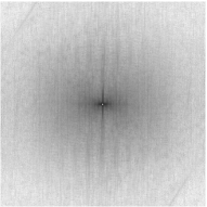
(a)                            (b)

(c)

Figure 1: Intensity plots of the longitudinal $S_{\ell\ell}(\vec{k})$ (a), and transverse $S_{tt}(\vec{k})$ (b), power spectra obtained from averaging over a set of 100 natural images. (c) Log-log plots of $S_{\ell\ell}({k})$ and $S_{tt}({k})$ after averaging over all angles.

The data in Fig. 1 clearly shows higher power in the transverse component. As with the intensities of natural images Ruderman94 , the power spectra are reasonably close to a power-law form $1/k^{2-\eta}$, presumably reflecting an underlying scale invariance since objects can appear at any distance from the viewer. (The straight line in Figs.1(c) corresponds to $\eta=0$.) We believe that the deviations from scale invariance (especially pronounced in the transverse component) are an artifact of our images. Converting intensity data to orientations involves filters with an inherent short distance scale; at such short scales the two power spectra coincide as required by local isotropy. There is a range of intermediate scales in which both spectra can be fitted to power laws. The deviations from scale invariance at shortest wavelengths are likely due to a tendency to frame photographs to include whole objects, excluding images with parts of objects extending beyond the frame global .

The enhanced transverse power is a consequence of the abundance of sharp and extended edges in natural images. An elementary illustration is obtained by comparing a long straight line with a horizontal arrangement of short vertical segments as in a fence. The former has no longitudinal Fourier component while the latter has weak transverse character. Searching for other sets of images with different statistics, we did a sampling of paintings from modern art. We find that many paintings from the impressionist school with blurred lines have approximately equal transverse and longitudinal powers. By contrast, cubist paintings with sharp lines share (and in fact exceed) the transversality of natural images WebData .

We next attempt to relate the above statistics to the lateral connections between neurons of V1, using information theoretic methods. The general idea is to construct an output signal by removing redundant correlations of the input signals as much as possible, maximizing the entropy of the output. Information theory has been used to describe early visual processing, such as the contrast response of large monopolar cellsLaughlin , the ‘center surrounded’ receptive fields in the retinaAtick1990 ; Atick1992 , and the white spatial/temporal power spectrum of signals from the LGNAtick1992 ; Dan . In Ref. Bialek , filters for processing intensity inputs to V1 were calculated by maximizing information subject to certain costs. Our approach is based on the latter, and as extended in Ref. Kardar , but employing an input signal which is an orientation field.

The response of simple cells in V1 is primarily to an oriented line in a preferred direction, which we shall approximate by ${\rm tr}[{\bf t}(\vec{x}){\bf s}(\vec{X})]=[\vec{t}(\vec{x})\cdot\vec{s}(\vec{X})]^{2}$. Here ${\bf s}_{\alpha\beta}(\vec{X})=s_{\alpha}(\vec{X})s_{\beta}(\vec{X})$ is constructed from the orientation of the image segment (input signal) at position $\vec{X}$ in the visual field, while a tensor ${\bf t}_{\alpha\beta}(\vec{x})\equiv t_{\alpha}(\vec{x})t_{\beta}(\vec{x})$ is defined in terms of the OP of a neuron at location $\vec{x}$ in V1. The topographic map between the visual field and V1 provides a mapping between $\vec{x}$ and $\vec{X}$. However, to emphasize that this mapping is not one to one, with many V1 neurons responding to signals at the same position in the visual field, we use two symbols $\vec{X}$ and $\vec{x}$.

Our main interest is in the lateral connections to a cell from other neurons in V1. With this aim, we indicate the net response (neuron firing rate), by

$$O(\vec{x})={\rm tr}[{\bf t}(\vec{x}){\bf s}(\vec{X})]+\int d^{2}yF(\vec{x},\vec{y}){\rm tr}[{\bf t}(\vec{y}){\bf s}(\vec{Y})]+\eta(\vec{x}).$$ (3)

The ‘filter function’ $F(\vec{x},\vec{y})$ denotes the strength of the horizontal connection between the neurons at $\vec{x}$ and $\vec{y}$; $\eta(\vec{x})$ is the noise experienced by the neuron which is assumed to be uncorrelated at different points, with $\langle\eta(\vec{x})\eta(\vec{x^{\prime}})\rangle=\sigma^{2}{\delta}^{2}(\vec{x}-\vec{x^{\prime}})$. Given the stochastic nature of the input signal (as well as the noise), the output $O(\vec{x})$ is a random variable with a (joint) probability distribution $p[O(\vec{x})]$. The associated Shannon information is

$$I=-\langle\ln p[O(\vec{x})]\rangle\approx{1\over 2}~{}{\mbox{ln}}~{}{\mbox{det}}[\langle O(\vec{x})O(\vec{x^{\prime}})\rangle_{c}],$$ (4)

where $\langle O(\vec{x})O(\vec{x^{\prime}})\rangle_{c}$ is the second cumulant (co-variance) of the output. The final approximation assumes a Gaussian $p[O(\vec{x})]$, and ignores higher order cumulants. For low signal to noise ratio we can further simplify the result to

$$I \approx {1\over 2}\int d^{2}\vec{x}~{}{\cal S}_{\alpha\beta\gamma\delta}(0)~{}{\bf t}_{\alpha\beta}(\vec{x}){\bf t}_{\gamma\delta}(\vec{x})$$

$$+ \int d^{2}\vec{x}\int d^{2}\vec{y}~{}F(\vec{x},\vec{y}){\cal S}_{\alpha\beta\gamma\delta}(\vec{X}-\vec{Y}){\bf t}_{\alpha\beta}(\vec{x}){\bf t}_{\gamma\delta}(\vec{y}),$$

where ${\cal S}_{\alpha\beta\gamma\delta}(\vec{X}-\vec{Y})=\langle{\bf s}_{\alpha\beta}(\vec{X}){\bf s}_{\gamma\delta}(\vec{Y})\rangle_{c}/\sigma^{2}$ denotes the co-variance of the input signal.

To provide a meaningful comparison of different filters, we need to maximize the above information subject to costs and constraints. In particular, it is reasonable to assume that an expansion of the wiring costs for small $F$ starts at quadratic order (so that no connections are formed in the absence of any gain). Following Refs. Bialek ; Kardar , we introduce a cost function

$$C[{\bf t},F]=C_{1}[{\bf t}]+{1\over 2}\int d^{2}\vec{x}d^{2}\vec{y}~{}C_{2}(\vec{x}-\vec{y})F(\vec{x},\vec{y})^{2},$$ (6)

where $C_{2}(r)$ is a cost for connecting neurons at a separation $r$. We would like to maximize $I-C$ with respect to both ${\bf t}(\vec{x})$ and $F(\vec{x},\vec{y})$. The largest contribution should come from the local OPs encoded in ${\bf t}(\vec{x})$. However, this is not our concern here, and for this reason we have not dwelled on the precise form of $C_{1}[{\bf t}]$. Given that the field ${\bf t}_{\alpha\beta}(\vec{x})$ has somehow been established, we would like to determine $F(\vec{x},\vec{y})$. Assuming that the latter connections provide a small correction to the overall information, maximization gives

$$F(\vec{x},\vec{y})={{{\bf t}_{\alpha\beta}(\vec{x}){\cal S}_{\alpha\beta\gamma\delta}(\vec{X}-\vec{Y}){\bf t}_{\gamma\delta}(\vec{y})}\over C_{2}(\vec{x}-\vec{y})}.$$ (7)

Figure 2: The strength of horizontal connections among neurons with parallel OPs (solid line $F_{||}$), and with orthogonal OPs (dotted line $F_{\perp}$), as a function of their angle $\varphi$ to the line between their locations in the visual field. The results are for a fixed separation, and obtained from the statistics of lines in a set of five images of trees.

The optimal connection between two V1 neurons thus depends on their OPs, and the correlations in natural signals at the corresponding locations and orientations. This qualitatively agrees with the observations in tree shrew Bosking97 and cat Nelson85 . To confirm that Eq. (7) does indeed predict the enhanced horizontal connections between colinear and co-oriented neurons, we measured the two point correlation functions by averaging over a set of five images of trees. Figure 2 compares the strength of the connection among neurons with parallel OPs ($F_{\parallel}$) to that of neurons with orthogonal OPs ($F_{\perp}$), as a function of the angle $\varphi$ between one of the OPs, and the line joining their locations in the visual field. The figure is for a constant separation $|\vec{x}-\vec{y}|$; the angular dependence is not very sensitive to this separation. There is a strong maximum in $F_{\parallel}$ at colinearity $\varphi=0$; while $F_{\perp}$ (which is always smaller than $F_{\parallel}$) shows weak maxima at $\pi/4$ and $3\pi/4$ (consistent with the co-circularity principleSigman ).

One advantage of optimal filters is observed by noting that the resulting noise-average output of a neuron is

$$O(\vec{x})={\bf t}_{\alpha\beta}(\vec{x})\left[{\bf s}_{\alpha\beta}(\vec{X})+\int d^{2}y\frac{\langle{\bf s}_{\alpha\beta}(\vec{X}){\bf s}_{\gamma\delta}(\vec{Y})\rangle_{c}}{C_{2}(\vec{x}-\vec{y})}{\bf s}_{\gamma\delta}(\vec{y})\right].$$

If the primary signal $s_{\alpha}(\vec{X})$ is somehow corrupted, the connections provide a guess based on global statistics. Let us employ similar principles to construct artificial algorithms for visual detection, which (like the human brain) are adept at deducing global shapes in an image composed of lines. As an alternative to Eq. (3) which avoids introduction of an OP field, we define a vectorial output whose components are

$$O_{\alpha}(\vec{x})=\int d^{2}y{\bf F}_{\alpha\beta}(\vec{x}-\vec{y})s_{\beta}(\vec{y})+\eta_{\alpha}(\vec{x}).$$ (8)

The filter is now a $2\times 2$ matrix. As in Eq. (1) its Fourier transform can be projected into longitudinal/transverse parts as

$${\bf F}_{\alpha\beta}(\vec{k})={\bf L}_{\alpha\beta}(\vec{k})F_{\ell}(\vec{k})+{\bf T}_{\alpha\beta}(\vec{k})F_{t}(\vec{k}).$$ (9)

Now consider a set of images in the form of a vector field $\vec{s}(\vec{x})$, which is statistically invariant under translations. For low signal to noise, the Shannon information in the output is

$$I={A\over 2}\int{d^{2}k\over{(2\pi)}^{2}}\left[|F_{\ell}(\vec{k})|^{2}S_{\ell\ell}(\vec{k})+|F_{t}(\vec{k})|^{2}S_{tt}(\vec{k})\right],$$ (10)

with projected signal correlations defined as in Eq. (9). As before, we can search for filters that maximize information subject to specified costs. However, to simplify matters we note that the transverse and longitudinal channels can be treated independently, and that most of the information is in the transverse channel which has the larger signal power spectrum. As such, we compared the performance of the following filters: (1) A transverse filter with $F_{t}(\vec{k})=\phi(k)$ and $F_{\ell}(\vec{k})=0$; and (2) an isotropic filter with $F_{t}(\vec{k})=F_{\ell}(\vec{k})=\phi(k)/\sqrt{2}$. In both cases, we chose $\phi(k)\propto\exp(-k^{2}/4C)$. The input image, illustrated in Fig. 3(a) consists of vectors, some pointing randomly (noise), and some arranged into a line with a gap (corrupted image). Figures 3(b)-(c) indicate how well the filters reconstruct the missing part. The output of the transverse filter is both stronger and better oriented to the erased line. (Detailed results quantifying the improvements shall be reported elsewhere.)

Figure 3: (a) A test image of a directed line with a gap (plus noise). Reconstructions of the missing segment, with an isotropic filter (b); and with a transverse filter (c).

The authors acknowledge support from the NSF grant DMR-01-18213 (MK); and by a University Postdoctoral Fellowship from The Ohio State University (HYL).

References

- (1) D. H. Hubel and T.N. Wiesel, J. Physiol. 160, 215 (1962).
- (2) M. Sigman, G. A. Cecchi, C. D. Gilbert, and M. O. Magnasco, Proc. Natl. Acad. Sci. USA 98, 1935 (2001).
- (3) D. J. Field, J. Opt. Soc. Am. A 4, 2379 (1987).
- (4) D. Ruderman and W. Bialek, Phys. Rev. Lett. 73, 814 (1994).
- (5) A. S. Monin and A. M. Yaglom, Statistical Mechanics (MIT, Cambridge, 1971), Vol. 2 pp. 1-58.
- (6) I. Arad, et. al, Phys. Rev. Lett. 81, 5330 (1998).
- (7) C. D. Gilbert and T. N. Wiesel, J. Neurosci. 9, 2432 (1989).
- (8) R. Malach, Y. Amir, M. Harel, and A. Grinvald, Proc. Natl. Acad. Sci. USA 90, 10469 (1993).
- (9) W. H. Bosking, Y. Zhang, B. Schofield, and D. Fitzpatrick, J. Neurosci. 17, 2112 (1997).
- (10) J. I. Nelson, and B. J. Frost, Exp. Brain Res. 61, 54 (1985).
- (11) Z. Kourtzi, et al., Neuron 37, 333 (2003).
- (12) S. B. Laughlin, Z. Naturf. 36c, 910 (1981).
- (13) J. J. Atick and A. N. Redlich, Neural Comput. 2, 308 (1990).
- (14) J. J. Atick, Network: Comput. Neural Sys. 3, 213 (1992).
- (15) Y. Dan, J. J. Atick, and R. C. Reid, J. of Neurosci. 16, 3351 (1996).
- (16) W. Bialek, D. L. Ruderman, and A. Zee, in Advances in Neural Information Processing Systems, R.P. Lippman, editor (Morgan Kaufmann, San Mateo, CA 1991), p. 363.
- (17) M. Kardar and A. Zee, Proc. Natl. Acad. Sci. USA 99, 15894 (2002).
- (18) S. Grossberg and E. Mingolla, Psychol. Rev. 92, 173 (1985).
- (19) J. H. van Hateren and A. Van der Schaaf, Proc. R. Soc. London B 265, 359 (1998).
- (20) W. T. Freeman and E. H. Adelson, IEEE Trans. Patt. Anal. Mach. Intell. 13, 891 (1991).
- (21) E. Switkes, M. J. Mayer, and J. A. Sloan, Vision Res. 18, 1393 (1978).
- (22) J. D. Pettigrew, T. Nikara, and P. O. Bishop, Exp. Brain Res. 6, 373 (1968).
- (23) B. Chapman and T. Bonhoeffer, Proc. Natl. Acad. Sci.USA 95, 2609 (1998).
- (24) V. Dragoi, C. M. Turch, and M. Sur, Neuron 32, 1181 (2001).
- (25) We confirmed that the spectra become more isotropic as we average over more rotated images. Note that with a matrix obtained from an orientation field, there is no a priori reason for the cross correlations and to be zero. We do find that these correlations are small, and also decrease as we average over rotated images.
- (26) This was tested by generating random lines within one frame. As the length of lines increases, the meeting point between the two spectra is shifted to smaller .
-
(27)
Additional pictures and data are available online from
http://www.mit.edu/kardar/research/transversality
/ModernArt/.