Analytical Solution of a Stochastic Content Based Network Model

Abstract

We define and completely solve a content-based directed network whose nodes consist of random words and an adjacency rule involving perfect or approximate matches, for an alphabet with an arbitrary number of letters. The analytic expression for the out-degree distribution shows a crossover from a leading power law behavior to a log-periodic regime bounded by a different power law decay. The leading exponents in the two regions have a weak dependence on the mean word length, and an even weaker dependence on the alphabet size. The in-degree distribution, on the other hand, is much narrower and does not show scaling behavior. The results might be of interest for understanding the emergence of genomic interaction networks, which rely, to a large extent, on mechanisms based on sequence matching, and exhibit similar global features to those found here.

PACS Nos: 87.10.+e,02.10.Ox,89.75.-k

I Introduction

In a previous paper, two of us (Balcan and Erzan) Balcan-Erzan introduced and numerically simulated a content based network Vespignani , with random binary strings associated with each node. The network arose by postulating a directed edge to exist between the nodes $i$ and $j$, if and only if the string, which can be regarded as a random word associated with the $i$th node, occurred at least once in the random word associated with the $j$th.

This stochastic network was shown Balcan-Erzan to display distinctly different topology than either the classical random networks of Erdös and Renyi Erdos or the “scale free” networks of the preferential-attachment universality class, introduced by Barabasi and Albert Barabasi1999 , Barabasi . Simulations Balcan-Erzan revealed that the in- and out-degree distributions, were markedly different, with in-degree distribution being rather localised. The out-degree distribution displayed a sharp crossover behavior. For small out-degree $d$, the distribution $n(d)$ exhibited a putative scaling behavior over a very narrow region, where the log-log plot could be fitted with a straight line with slope $-\gamma_{1}\simeq-1$, whereas, for larger $d$, log-periodic oscillations were found, with an envelope which could again be fitted, on a double logarithmic plot, by a linear graph with a slope $-\gamma_{2}\simeq-1/2$.

The purpose of this paper is twofold. We first extend the model of Balcan and Erzan Balcan-Erzan to a broader class of models in which the random strings are derived from an $r+1$ letter alphabet and where partial matches are allowed. Second, we obtain analytical expressions for the ensemble averaged in- and out-degree distributions and investigate the crossover behavior of the out-degree distribution. We show that the putative scaling behavior observed in the simulations to coincides with the leading power law behavior obtained from our analytical results. We describe in detail the finite size corrections to the infinite network limit. Comparison of our analytical predictions with the numerical data Balcan-Erzan for the $r=2$ random bit string model with perfect matches shows very good agreement.

The paper is organized as follows: In the next section we reformulate the random string model of Balcan-Erzan for an alphabet of $r+1$ letters. Our analytical results depend on the matching probability $p(l,k)$ that a string of length $l$ selected randomly from the set of all strings of length $l$ is contained at least once in a string of length $k$, $k\geq l$, that has been selected randomly from the set of all strings of length $k$. In Section III we derive an approximate form for this probability that is valid for moderately long strings $k\lesssim r^{l}$ and that allows for partial matches. Using the results of Section III, we obtain in Section IV analytical expressions for the in- and out-degree distributions. We investigate the scaling behavior of the out-degree distribution in these models and compare our results with the numerical data of Balcan-Erzan . We conclude this paper with a discussion of the possible relevance of our results to genomic networks, in Section V.

II The Random String Model

Consider a random sequence $C$ of fixed length $L$, consisting of letters from an alphabet $A$ of $r+1$ letters. The elements of the sequence $C$, $x\in\{0,1,\ldots,r\}$ are assumed to be independently and identically distributed according to

$$P(x)=p\delta(x-r)+(1-p)\frac{1}{r}\sum_{m=0}^{r-1}\delta(x-m)\;\;.$$ (1)

A subsequence $G_{i}$ of $C$, composed of the letters $\{0,\ldots,r-1\}$ only, sandwiched between the $i^{th}$ and $(i+1)^{th}$ occurrences of the letter “$r$,” will be denoted the $i$th “random word,” or “string,” and will be associated with the $i$th vertex of a graph. For convenience, we assume that a letter “$r$” has also been placed at the $0^{th}$ and $(L+1)^{th}$ positions. With these definitions, the $i^{th}$ string can be written,

$$G_{i}=x_{i,1},x_{i,2},\ldots,x_{i,\ell_{i}},\ \ i=1,2,\ldots,N$$ (2)

where $N$ is the number of strings (equivalently, vertices), the “letter” $x_{i,\lambda}\in\{0,r-1\}$, $\lambda=1,\ldots,\ell_{i}$, and $\ell_{i}$ is the length of the $i^{th}$ string $G_{i}$. Let $n_{\ell}$ be the number of strings of length $\ell$ and $q=1-p$. It follows that

$$\sum_{i}{\ell_{i}}=L-N\ ,\ \ \ \sum_{\ell}{n_{\ell}}=N\ ,$$ (3)

$$\langle\ell\rangle=p^{-1}-1,\ \ \ \langle n_{\ell}\rangle=Lp^{2}q^{\ell},\ \ \ \langle N\rangle=Lp.$$ (4)

Unless noted otherwise, we will assume that $L$ and $Lp$ are sufficiently large so that fluctuations in the number and length of the strings for different realizations of the random sequence $C$ can be neglected when calculating statistical properties of quantities of interest. We will also discard the cases with $\ell=0$ and construct the graph from the remaining vertices. The adjacency matrix is defined by the matching condition

$$w_{ij}=\begin{cases}1&G_{i}\subset G_{j},\\ 0&\text{otherwise}.\end{cases}$$ (5)

By $G_{i}\subset G_{j}$ we mean that there exists an integer $\lambda$ such that $0\leq\lambda\leq\ell_{j}-\ell_{i}$ and

$$x_{i,l}=x_{j,\lambda+l},\ \ l=1,\ldots,\ell_{i}.$$ (6)

Two vertices are said to be connected if the string $G_{i}$ appears as a subsequence of $G_{j}$, or in other words $G_{j}$ matches $G_{i}$. Thus $w_{ij}=1$ indicates a directed link (an edge) from $G_{i}$ to $G_{j}$. We will also consider imperfect matches, where Eq. (6) is valid only for some values of $l$ rather than all values. In order to avoid ambiguity we will refer to the former case as a perfect match. For $Lp$ large enough ($p>p_{c}(L)$, see Balcan-Erzan ), which is assumed here, the graph consists of one giant cluster. We will henceforth refer to this graph as the network, and denote the vertices, or equivalently, the strings associated with them, as the “nodes.”

The resulting network was numerically studied earlier by Balcan and Erzan in Balcan-Erzan , for the case of binary strings, i.e., $r=2$, and perfect matches Eq. (6), where it was shown that the logarithm of the out-degree distribution behaved linearly over a very narrow, initial range, with a slope of $\simeq-1$. Beyond a crossover point the distribution exhibited an oscillatory behavior, whose envelope again behaved linearly on a log-log plot, with a different slope, namely $\simeq-1/2$. The out-degree distribution is shown in Figure (1), where the numerical results were obtained Balcan-Erzan by averaging the out-degree distributions over 500 graphs, associated with independently generated sequences of length $L=15000$, and $p=0.05$. Notice the strong oscillatory behavior. It turns out that each peak in the out-degree distribution is supported predominantly by the out-degrees of genes with a corresponding common length $l$.

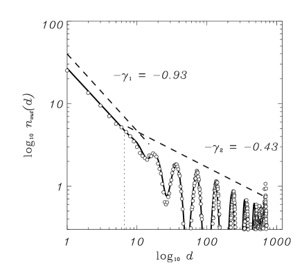
Figure 1: Scaling behavior of the out-degree distribution. The numerical data (circles) shows a cross-over in the scaling behavior from small values of the out-degree to larger values. The solid line is the theoretical expression. The dashed lines serve as a guide to the eye for the predicted scaling behavior and have been offset for clarity. The cross-over occurs at $d_{c}=6.6$ and has been shown as a vertical line.

In order to proceed with the analytical treatment, it is convenient to group the $G_{i}$ into subsets according to their lengths and we define

$${\cal G}_{l}=\{G_{i}|\ell_{i}=l\}\ .$$ (7)

It turns out that that the central quantity determining the behavior of the in- and out-degree distributions is the probability $p(l,k)$ that a string in ${\cal G}_{l}$ has an outgoing edge terminating in a member of ${\cal G}_{k}$. We therefore turn next to the derivation of $p(l,k)$. The discussion of the degree distributions will then be taken up in Section IV.

III Analytical Results for the Matching Probability

Let $x$, and $y$ be variables such that $x,y,\in\{0,\ldots,r-1\}$. Define an interaction $u(x,y)$ between $x$ and $y$ as

$$u(x,y)=1-\delta(x-y).$$ (8)

Let ${\bf x}=(x_{1},x_{2},x_{3},\ldots,x_{l})$ and ${\bf y}=(y_{1},y_{2},y_{3},\ldots,y_{l})$, be two strings of $l$ letters and define their interaction $U({\bf x},{\bf y})$ as

$$U({\bf x},{\bf y})=\sum_{t=1}^{l}u(x_{t},y_{t}).$$ (9)

The function $U({\bf x},{\bf y})$, as defined above, counts the number of unmatched letters between strings ${\bf x}$ and ${\bf y}$.

Introduce an “inverse temperature” $\beta$ and consider the Boltzmann factor $e^{-\beta U}$. In the “zero temperature” limit we have

$$\lim_{\beta\rightarrow\infty}e^{-\beta U({\bf x},{\bf y})}=\left\{\begin{array}[]{ll}1,&\mbox{if ${\bf x}={\bf y}$}\\ 0,&\mbox{otherwise}.\end{array}\right.$$ (10)

We see that the limit $\beta\rightarrow\infty$ is a “no tolerance” limit Ozcelik , enforcing perfect matching of x and y, i.e. $x_{t}=y_{t}$, $t=1,2,\ldots,l$. Let ${\bf y}=(y_{1},y_{2},\ldots,y_{k})$ be a string of length $k\geq l$ and denote by ${\bf y}_{a,l}=(y_{a+1},y_{a+2},\ldots,y_{a+l})$ the substring of length $l$ starting at position $a$, $a=0,1,\ldots,k-l$. Furthermore let

$$f_{a}({\bf x},{\bf y};\beta)=e^{-\beta U({\bf x},{\bf y}_{a,l})}.$$ (11)

so that we have

$$f_{a}({\bf x},{\bf y})\equiv\lim_{\beta\rightarrow\infty}f_{a}({\bf x},{\bf y};\beta)=\left\{\begin{array}[]{ll}1,&\mbox{${\bf x}={\bf y}_{a,l}$ }\\ 0,&\mbox{otherwise}.\end{array}\right.$$ (12)

Thus, $f_{a}({\bf x},{\bf y})=1$, if and only if ${\bf x}$ matches ${\bf y}$ at position $a$, and zero otherwise.

Likewise, let $f({\bf x},{\bf y})$ be a function that takes on the value one if the $k$-string ${\bf y}$ contains the given $l$-string ${\bf x}$ and zero otherwise. Note that the complement of the event that ${\bf x}$ matches ${\bf y}$ is the event that ${\bf x}$ does not match ${\bf y}$ anywhere. Thus, using Eq. (12), we can write

$$f({\bf x},{\bf y})=1-\prod_{a=0}^{k-l}\left[1-f_{a}({\bf x},{\bf y})\right].$$ (13)

Letting $p(l,k;{\bf x})$ denote the probability that a randomly drawn $k$-string ${\bf y}$ contains a given $l$-string ${\bf x}$, we therefore find

$$p(l,k;{\bf x})=1-\frac{1}{r^{k}}\sum_{{\bf y}}\prod_{a=0}^{k-l}\left[1-f_{a}({\bf x},{\bf y})\right],$$ (14)

where $r^{k}$ is the number of distinct $k$-strings of $r$-letters, and $\sum_{{\bf y}}$ denotes the sum over all such strings ${\bf y}$.

Generalizing the above equation to incorporate partial matches we obtain:

$$p(l,k;{\bf x})=\lim_{\beta\rightarrow\infty}p(l,k;{\bf x},\beta),$$ (15)

where

$$p(l,k;{\bf x},\beta)=1-\frac{1}{r^{k}}\sum_{{\bf y}}\prod_{a=0}^{k-l}\left[1-f_{a}({\bf x},{\bf y};\beta)\right].$$ (16)

The products in equation (16) can be expanded and we obtain a Mayer-like sum

$$p(l,k;{\bf x},\beta) = \frac{1}{r^{k}}\sum_{{\bf y}}\sum_{a}f_{a}-\frac{1}{r^{k}}\sum_{{\bf y}}\sum_{a<b}f_{a}f_{b}$$ (17)

$$+ \frac{1}{r^{k}}\sum_{{\bf y}}\sum_{a<b<c}f_{a}f_{b}f_{c}-\ldots,$$

which we can write as

$$p(l,k;{\bf x},\beta) = \sum_{a}W^{(1)}(a;{\bf x})-\sum_{a<b}W^{(2)}(a,b;{\bf x})$$ (18)

$$+ \sum_{a<b<c}W^{(3)}(a,b,c;{\bf x})-\ldots,$$

where

$$W^{(1)}(a;{\bf x}) = \frac{1}{r^{k}}\sum_{{\bf y}}f_{a}({\bf x},{\bf y};\beta)$$

$$W^{(2)}(a,b;{\bf x}) = \frac{1}{r^{k}}\sum_{{\bf y}}f_{a}({\bf x},{\bf y};\beta)f_{b}({\bf x},{\bf y};\beta)$$

$$W^{(3)}(a,b,c;{\bf x}) = \frac{1}{r^{k}}\sum_{{\bf y}}f_{a}({\bf x},{\bf y};\beta)f_{b}({\bf x},{\bf y};\beta)f_{c}({\bf x},{\bf y};\beta)$$ (19)

$$\cdots$$

Using equations (8) and (11), we obtain

$$W^{(1)}(a;{\bf x})=\frac{1}{r^{l}}\left[1+(r-1)e^{-\beta}\right]^{l}\equiv W^{(1)}.$$ (20)

Note that $W^{(1)}(a;{\bf x})$ is independent of $a$, and ${\bf x}$.

Let us now turn to the second order term, $W^{(2)}(a,b;{\bf x})$ in Eqs. (18) and (19). Here, we need to distinguish two cases, (i) $b-a\geq l$ and (ii) $b-a<l$.

In case (i), the set of indices of ${\bf y}_{a,l}$ and ${\bf y}_{b,l}$ are distinct and the evaluation of the partition sum proceeds analogously to equation (20) yielding

$$W^{(2)}(a,b;{\bf x})=\left(\frac{1}{r^{l}}\right)^{2}\left[1+(r-1)e^{-\beta}\right]^{2l},\,|b-a|\geq l.$$ (21)

In case (ii), $|b-a|<l$, there is an overlap between the indices of ${\bf y}_{a,l}$ and ${\bf y}_{b,l}$. Letting $|b-a|=m$, we find

$$W^{(2)}(a,b;{\bf x})=\frac{1}{r^{l+m}}\left[1+(r-1)e^{-\beta}\right]^{2m}$$

$$\times\prod_{t=1}^{l-m}\left[1+(r-1)e^{-2\beta}-u(x_{t},x_{m+t})\left(1-e^{-\beta}\right)^{2}\right],$$

$$|b-a|<l.$$ (22)

Note that $W^{(2)}(a,b;{\bf x})$, as defined Eqs. (21) and (22), depends on ${\bf x}$ only when $|b-a|<l$. Next, we perform the ${\bf x}$ average of $W^{(2)}(l,k;\bf{x})$,

$$\frac{1}{r^{l}}\sum_{{\bf x}}W^{(2)}(a,b;{\bf x})=\frac{1}{r^{2l}}\left[1+(r-1)e^{-\beta}\right]^{2l}.$$ (23)

The calculations leading to Eqs. (22) and (23) are a little involved and can be found in the appendix.

Comparing Eqs. (20) and (23), we see that once averaged over ${\bf x}$, $W^{(2)}$ factorizes as

$$W^{(2)}=\left<W^{(2)}(a,b;{\bf x})\right>_{x}=\left(W^{(1)}\right)^{2},$$ (24)

or equivalently,

$$\left<f_{a}f_{b}\right>_{y,x}=\left<f_{a}\right>_{y,x}\left<f_{b}\right>_{y,x},\ \ \ a\neq b,$$ (25)

where, for simplicity, we have introduced the short hand notation $\left<\ldots\right>_{y,x}$ to denote averaging first over ${\bf y}$ then ${\bf x}$.

Let us therefore make the approximation that all higher moments factorize similarly,

$$\left<f_{a_{1}}f_{a_{2}}\ldots f_{a_{s}}\right>_{y,x}\simeq\left<f_{a_{1}}\right>_{y,x}\left<f_{a_{2}}\right>_{y,x}\ldots\left<f_{a_{s}}\right>_{y,x},$$ (26)

with $\{a_{s}\}$ being distinct. It can be readily shown that Eq. (26) is exact when $a_{i+1}-a_{i}>l$, i.e, there are no overlaps between the segments at position $a_{i}$. Upon substituting Eq. (26) into Eq. (17) and performing the ${\bf x}$ average we obtain the matching probability

$$p(l,k;\beta)=\left<p(l,k;{\bf x},\beta)\right>_{x},$$ (27)

with

$$p(l,k;\beta)=1-\left(1-\frac{1}{r^{l}}\left[1+(r-1)e^{-\beta}\right]^{l}\right)^{k-l+1}.$$ (28)

In the “zero temperature” limit ($\beta\rightarrow\infty$), this becomes

$$p(l,k)=1-\left(1-\frac{1}{r^{l}}\right)^{k-l+1}.$$ (29)

For $r^{l}\gg k$, $p(l,k;\beta)$ has the asymptotic form

$$p(l,k;\beta)=1-\exp{\left(-\frac{k-l+1}{r^{l}}\left[1+(r-1)e^{-\beta}\right]^{l}\right)},$$ (30)

which for $\beta\rightarrow\infty$ becomes

$$p(l,k)=1-\exp{\left(-\frac{k-l+1}{r^{l}}\right)}.$$ (31)

For very large $l$ this further reduces to

$$p(l,k)={\frac{k-l+1}{r^{l}}}.$$ (32)

Note that a finite $\beta$ acts like an enhanced matching probability, i.e., a false positive match. In the limit $\beta\rightarrow 0$, the matching probability becomes

$$\lim_{\beta\rightarrow 0}p(l,k;\beta)=1$$ (33)

Hence the “high-temperature” limit of our model corresponds to indiscriminate matches.

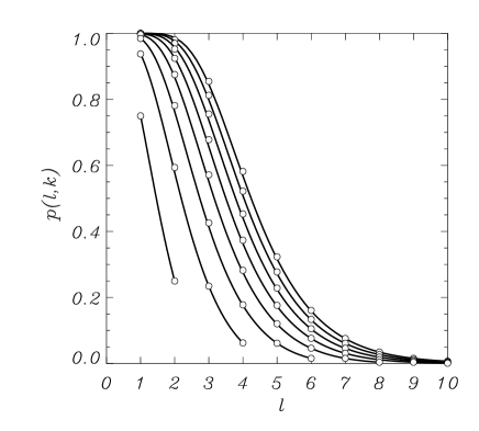
Figure 2: Comparison of the exact matching probability $p(k,l)$ (circles) with the approximate expression (29) (lines) for $r=2$ and perfect matches. The curves are (from top to bottom) for values of $k=16,14,12,10,8,6,4,2$.

Of course, the crucial approximation, Eq. (26), is not correct in general and one expects corrections coming from higher order correlations contained in Eq. (18). These correlations are due to the fact that if a given string ${\bf x}$ is matched at a position $a$, this affects the likelihood of matching the same string at any nearby location $b$ with $|b-a|\lesssim l$. Nevertheless, the approximate result for $p(l,k)$, Eq. (29), is surprisingly good. Fig. (2) shows a comparison of the matching probability obtained from exact enumeration carried out computationally, with the analytical expression (29) for $r=2$ and perfect matches. As can be seen from the figure, there are only very small discrepancies for small $l$ when $k>2^{l}$, e.g. data points around $k=16,14,12$ with $l=4,3,2$. Since our expression for $p(l,k)$, Eq. (29), is exact for $l=1$, there are no discrepancies at $l=1$.

Notice that Eq. (32) is the matching probability that can alternatively be obtained by assuming the probabilities of matching a string of length $l$ at any position in a string of length $k$ are independent, and equal, $1/r^{l}$. Eq. (29), on the other hand, is the matching probability that can also be found assuming the probabilities of not matching a string of length $l$ at any position in a string of length $k$ are independent and equal, $1-1/r^{l}$. Thus the factorization approximation, Eq. (26), leading to Eq. (28) implies that the probabilities of not matching at a given position are independent.

For the regime of interest, $k\lesssim 2^{l}$, this approximation leading to Eq. (29) is extremely good. We think that this is due to the fact that the factorization property underlying our approximation, Eq. (26), is exact for the two-point correlation function ($s=2$), Eq. (24). This means that any corrections to this result must be coming from higher order correlations with strongly overlapping segments, since non-overlapping segments will factorize and thus reduce to lower order correlators. This is very similar to the connected cluster expansion in statistical mechanics StatMechBooks . Indeed, such an expansion can be set up, however the calculations are rather tedious due to the discreteness of the problem and beyond the scope of this paper. Yet it is clear that the weight of an $s$-point correlation function with $s$ overlapping (connected) segments must be very small for large $s$, since the overlap imposes very strong conditions on the structure of the string ${\bf x}$ to be matched.

For the remainder of the paper it is convenient to define the quantities $t$ and $z$ as

$$t = 1-\frac{1}{r^{l}}\left[1+(r-1)e^{-\beta}\right]^{l}=1-z^{l}$$ (34)

$$z = \frac{1}{r}\left[1+(r-1)e^{-\beta}\right],$$ (35)

where we have suppressed the $\beta$, $r$ and $l$ dependence for clarity. Notice that the effect of the number of letters in the alphabet $r$ and the extent of mismatch as parametrized by the “inverse temperature” $\beta$ enter into the expression for $p(l,k;\beta)$ as a single parameter, $z$, as defined above. With the above definitions, Eq. (28) becomes

$$p(l,k;z)=1-t^{k-l+1}=1-\left(1-z^{l}\right)^{k-l+1}.$$ (36)

The “zero-temperature” limit is given by $z=r^{-1}$, while the “high-temperature” limit is $z=1$. The range of $z$ is therefore, $z\in(r^{-1},1)$, which for $r\gg 1$, approaches $z\in(0,1)$.

We note in passing that the matching probability computed in this section, is in a sense complementary to the problem of sequence alignment Karlin0 , Karlin1 , which has important applications in the study of proteins and DNA. The problem there is to identify subsequences of arbitrary length, showing strong similarity beyond pure statistical chance, within two long sequences sampling the same alphabet, possibly with different native probabilities. The pioneering work of Altschul, Karlin, et al. Karlin0 , Karlin1 yields a probability distribution for the similarity score of such likely regions, under the assumption that the region with the highest score is unique (i.e., non-degenerate), that the two sequences searched are of comparable length, and sufficiently long. The scoring scheme is to a large extent arbitrary as long as the scores corresponding to some degree of matching are rare (and positive) while those corresponding to mismatches are much more probable (and negative). This arbitrariness may be removed by proper normalization and scores obtained via different schemes can be compared in a meaningful way. The matching probability computed in the present paper could be related to the probability for the highest score (corresponding to an exact match without gaps), holding for the entire length of the shorter sequence. However, our calculation makes no assumptions regarding the relative lengths of the two sequences, apart from the obvious requirement that $l\leq k$. The approximation to which we have to resort in the final solution works best when either the two sequences are almost of the same length, or if $k\lesssim r^{l}$. Moreover there is no assumption regarding the number of times the highest score is achieved. More interestingly, the statistics of multiple high-scoring segments Karlin2 could have been related to the out-degree statistics of a given node had we taken each high scoring match in the complete random sequence to correspond to a different edge. As it is, a single edge corresponds to the presence of one or more occurrences of a shorter string, say $G_{i}$, inside a longer string $G_{j}$. That is, multiple occurrences of the shorter string within a subsequence of the complete random sequence are bunched together to result in a single edge between the nodes $i$ and $j$.

We now turn to the calculation of the in- and out-degree distributions.

IV The Degree Distributions

In Section II we showed that the subsequences $\{G_{i}\}$ of a random sequence $C$ generate a network whose nodes are associated with these strings, and whose edges are defined by the matching relation Eq. (5). In this section we will derive the in- and out-degree distribution associated with this network.

Consider a randomly selected string $G_{i}$. The in- and out-degree of the corresponding node, $d_{\rm in}(i)$ and $d_{\rm out}(i)$, are defined by the total number of edges terminating in and originating from that node, respectively,

$$d_{\rm in}(i) = \sum_{j}w_{ji}$$

$$d_{\rm out}(i) = \sum_{j}w_{ij}.$$ (37)

The corresponding in- and out-degree distributions are given by

$$n_{\rm in}(d) = \sum_{i}\delta\left(d-d_{\rm in}(i)\right)$$

$$n_{\rm out}(d) = \sum_{i}\delta\left(d-d_{\rm out}(i)\right).$$ (38)

IV.1 The Out-Degree Distribution

Letting ${\cal G}_{l}$ denote the set of strings of length $l$, we can rewrite the out-degree distribution Eq. (38) as

$$n_{\rm out}(d)=\sum_{l=1}^{L}n_{l}\left[\frac{1}{n_{l}}\sum_{j\in{\cal G}_{l}}\delta\left(d-d_{\rm out}(j)\right)\right].$$ (39)

For large $n_{l}$, the quantity in parentheses will approach the (conditional) probability $P_{\rm out}(X_{l}=d|l)$ that a randomly selected string whose length is given to be $l$ has an out-degree $d$.

In the limit $L,N\rightarrow\infty$, such that $N/L=p$, the ratio of the number of strings, $N$, to the length of the whole random sequence, $L$, remains constant, all the possible $r^{l}$ realizations of random words of a given length $l$ will be present with equal respective weights and we have,

$$\lim_{L,N\rightarrow\infty}\frac{1}{n_{l}n_{k}}\sum_{i\in{\cal G}_{l}}\sum_{j\in{\cal G}_{k}}w_{ij}=p(l,k).$$ (40)

We will refer to this limit as the large-$L$ limit.

The quantity $p(l,k)$, as defined in the above equation, is the probability that a randomly selected string of given length $l$ matches another independently and randomly selected string of length $k$. This probability has been calculated in Section III for the general case of imperfect matches, Eq. (28), as well as perfect matches, Eq. (29). Eqs. (39) and (40) show the self-averaging property of the degree distribution in the large-$L$ limit.

Define the random variable $X_{lk}$, as the number of edges originating from a randomly selected string of length $l$ that terminate in strings of length $k$. Then $X_{l}$ can be written as a sum of the random variables $X_{lk}$,

$$X_{l}=\sum_{k\geq l}X_{lk}.$$ (41)

We can therefore write $X_{l}$ as

$$\langle X_{l}\rangle=\frac{1}{n_{l}}\sum_{i\in{\cal G}_{l}}\sum_{k=l}^{L}\sum_{j\in{\cal G}_{k}}w_{ij},$$ (42)

or,

$$\langle X_{l}\rangle=\sum_{k=l}^{L}n_{k}\left[\frac{1}{n_{l}n_{k}}\sum_{i\in{\cal G}_{l}}\sum_{j\in{\cal G}_{k}}w_{ij}\right].$$ (43)

We see from Eqs. (43) and (40) that in the large-$L$ limit

$$\left<X_{lk}\right>=n_{k}p(l,k),$$ (44)

and

$$\left<X_{l}\right>=\sum_{k=l}^{L}n_{k}p(l,k),$$ (45)

where $\left<\cdots\right>$ denotes an average over all the strings of length $l$ in the complete random sequence. Note that in the large-$L$ limit $X_{lk}$ is binomially distributed,

$$P(X_{lk}=d|l)=\left(\begin{array}[]{ll}n_{k}\\ d\end{array}\right)p(l,k)^{d}\left(1-p(l,k)\right)^{n_{k}-d}.$$ (46)

As can be seen from Eq. (41), $X_{l}$ is a sum of the random variables $X_{lk}$ and thus in the large-$L$ limit the central limit theorem assures that the distribution for $X_{l}$ will approach a Gaussian distribution,

$$P_{\rm out}(X_{l}=d|l)=\frac{1}{\sqrt{2\pi}\sigma_{l}}\exp\left[-\frac{(d-d_{l})^{2}}{2\sigma_{l}^{2}}\right],$$ (47)

whose mean $d_{l}$ and standard deviation $\sigma_{l}$ are given by those of $X_{lk}$, Eq. (41), according to:

$$d_{l} = \left<X_{l}\right>=\sum_{k\geq l}\left<X_{lk}\right>$$ (48)

$$\sigma_{l}^{2} = \left<X_{l}^{2}\right>-\left<X_{l}\right>^{2}=\sum_{k\geq l}\left<\sigma_{lk}^{2}\right>,$$ (49)

where

$$\sigma_{lk}^{2}=\left<X_{lk}^{2}\right>-\left<X_{lk}\right>^{2}.$$ (50)

For binomially distributed $X_{lk}$ we have

$$\left<X_{lk}\right> = n_{k}p(l,k)$$ (51)

$$\sigma_{lk}^{2} = n_{k}p(l,k)\left(1-p(l,k)\right).$$ (52)

Using Eq. (36), one can readily carry out the sums in Eqs. (48) and (49) to find

$$d_{l} = \frac{N}{p+qz^{l}}\left(qz\right)^{l}$$ (53)

$$\sigma_{l}^{2} = d_{l}\frac{pt}{1-qt^{2}}.$$ (54)

Noting also that the probability of selecting a string of length $l$ is $pq^{l}$, the total out-degree distribution is given by

$$P_{\rm out}(d)=\sum_{l=1}^{L}pq^{l}P_{out}(X_{l}=d|l).$$ (55)

and thus in the large-$L$ limit we obtain

$$P_{\rm out}(d)=\sum_{l=1}^{L}pq^{l}\frac{1}{\sqrt{2\pi}\sigma_{l}}\exp\left[-\frac{(d-d_{l})^{2}}{2\sigma_{l}^{2}}\right]$$ (56)

with $d_{l}$ and $\sigma_{l}$ given by Eqs. (53) and (54), respectively.

As $l$ becomes large, $p(l,k)$ decreases towards zero. Thus with increasing $l$ the binomial distribution of $X_{lk}$, Eq. (46), will approach a Poisson distribution of the same mean. Note that the sum of independent and Poisson distributed random variables is also Poisson distributed with mean equal to the sum of the individual means. Thus for large $l$, $X_{l}$ as defined in Eq. (41), is Poisson. For a Poisson distributed random variable the variance equals to its mean so that for large $l$ we expect

$$\sigma^{2}_{l}=d_{l}\;\;,$$ (57)

as can also be directly verified by taking the appropriate limit in Eq. (54).

IV.1.1 Ensemble Averages and Finite Size Effects

The numerical data of Balcan-Erzan has been obtained from averaging over 500 realizations of a random sequence of length $L=15000$ with $N=750$. A finite sample size will cause sample to sample fluctuations in the number of strings, or “random words.” An average over a large ensemble of different realizations will yield the same average values for the out-degrees as those obtained from a single random sequence of infinite length. However averaging over many realizations will increase the fluctuations around the mean. It is not hard to see that this will affect predominantly nodes with large out-degrees, (short strings) where there is already self-averaging within the random sequence, but with a distribution which varies from sample to sample.

Nodes with small out-degrees (long strings) correspond to rare matches and thus for these nodes there is no self-averaging within the sample. To see this, consider the extreme case, where a sample contains on average one or less matches for such a node. When an ensemble average is taken, the dominant contribution to the variance of the out-degree will come from the sample to sample fluctuations.

Denoting the mean and variance of the out-degree of a node of length $l$, that has been corrected for the finite size, by $\tilde{d}_{l}$ and $\tilde{\sigma}^{2}_{l}$, respectively, we have

$$\tilde{d}_{l}=d_{l},\ \ \tilde{\sigma}^{2}_{l}\rightarrow\sigma^{2}_{l}\ \ \ \mbox{for large $l$}.$$ (58)

In what follows we will re-calculate previously introduced statistics, taking into account the fluctuations in $n_{k}$. In order to avoid confusion, these quantities will be denoted with a tilde.

We can estimate $\tilde{\sigma}^{2}_{l}$ as follows. The random variable $\tilde{X}_{lk}$ itself is a sum of random variables:

$$\tilde{X}_{lk}=\sum_{j\in{\cal G}_{k}}Y_{lj},$$ (59)

where $Y_{lj}=1$ if the string $G_{j}$ of length $k$ matches the (given) string of length $l$ and zero otherwise. Such an event constitutes a Bernoulli trial and its probability is $p(l,k)$. The mean and variance of $Y_{lj}$ are given by

$$\langle Y_{lj}\rangle = p(l,k)$$ (60)

$$\langle Y^{2}_{lj}\rangle-\langle Y_{lj}\rangle^{2} = p(l,k)(1-p(l,k))$$ (61)

The number of such trials is $\tilde{n}_{k}$, the number of elements of ${\cal G}_{k}$, and hence $\tilde{n}_{k}$ itself is a random variable. For sufficiently large $N$ and for values of $\tilde{n}_{k}$ near the mean, the constraints, Eq. (4), can be neglected and the probability of finding $\tilde{n}_{k}$ strings of length $k$ is approximately binomially distributed

$$P(\tilde{n}_{k}=n)=\left(\begin{array}[]{ll}N\\ n\end{array}\right)\left(pq^{k}\right)^{n}\left(1-pq^{k}\right)^{N-n}.$$ (62)

We thus find

$$\langle\tilde{n}_{k}\rangle = Npq^{k}$$ (63)

$$\tilde{\sigma}^{2}_{n_{k}} = pq^{k}(1-pq^{k}).$$ (64)

Finding the distribution of a sum over a finite random number $n$ of independently distributed random variables $Y$ can be readily worked out using moment generating functions (see for example Feller Feller ). In the case when both $\tilde{n}_{k}$ and $Y_{lj}$ are binomial it turns out that the resulting distribution is binomial again, and we find

$$P(\tilde{X}_{lk}=d|l)=\left(\begin{array}[]{ll}N\\ d\end{array}\right)\left[pq^{k}p(l,k)\right]^{d}\left[1-pq^{k}p(l,k)\right]^{N-d},$$ (65)

with mean and variance

$$\left<\tilde{X}_{lk}\right> = Npq^{k}p(l,k)$$ (66)

$$\tilde{\sigma}^{2}_{lk} = Npq^{k}p(l,k)\left[1-pq^{k}p(l,k)\right].$$ (67)

Thus Eq. (65) is the finite size result replacing Eq. (46), which is valid in the large-$L$ limit. As remarked before, the means of the two distributions in Eqs. (48) and (66) are equal, i.e., $\left<\tilde{X}_{lk}\right>=\left<X_{lk}\right>$. However, the variances are different and $\sigma^{2}_{lk}<\tilde{\sigma}^{2}_{lk}$. Note that the second term in Eq. (67) is of the order of $(1-p)\approx 1$ for small $p$. Thus we find to order $p$

$$\tilde{\sigma}^{2}_{lk}=\left<\tilde{X}_{lk}\right>,$$ (68)

and consequently to this order the mean and variance of $\tilde{X}_{l}$ become

$$\tilde{\sigma}^{2}_{l}=\left<\tilde{X}_{l}\right>=\left<X_{l}\right>=d_{l},$$ (69)

where $d_{l}$ is the same mean out-degree that was previously obtained in the large $L$-limit, Eq. (53). The out-degree distribution corrected for finite-size effects thus becomes, c.f., Eq. (56),

$$\tilde{P}_{\rm out}(d)=\sum_{l=1}^{L}pq^{l}\frac{1}{\sqrt{2\pi d_{l}}}\exp\left[-\frac{(d-d_{l})^{2}}{2d_{l}}\right].$$ (70)

Comparing this expression with the distribution obtained in the large-$L$ limit, Eq. (56), we find that finite size corrections are only present for small $l$, since we have already shown that the relation $d_{l}=\sigma^{2}_{l}$ is also valid (viz. Eq. (57)) in the large $l$ region for the large-$L$ case. Figure (3) shows a comparison of the numerically obtained out-degree distribution (circles) with the theoretical expressions with and without finite size corrections. The solid line is the analytical result for the out-degree distribution, Eq. (70), that takes into account finite size corrections, while the dotted line corresponds to the case where the network is assumed to be self-averaging, i.e., Eq. (56) is satisfied, and thus sample to sample fluctuations can be neglected. Note the large difference from the observed behavior for $l<6$, ($d>200$) in the height and broadness of the distributions, when finite size effects are not taken into account. The agreement of the finite size corrected distribution with the numerical data, on the other hand, is rather good, and we conclude that finite size effects present in the numerical data for short nodes are satisfactorily accounted for.

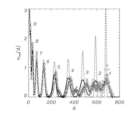
Figure 3: Comparison of the theoretical out-degree distributions with numerical data (circles). The dotted line shows the theoretical result for a network in the large $L$-limit, where the network is self-averaging and thus all possible realizations of a string of a given length $l$ can be found. The number to the right of each peak refers to the node length $l$ that contributes predominantly to that peak. The solid line is obtained after correcting for finite size effects (see text for details). In both cases, the locations of the peaks are accurately predicted. Note that the results for the large-$L$ limit differ strongly in their predictions for the width and height of each peak for small $l$, (large $d$). It is evident that the numerical data exhibits finite size effects for short nodes, $l\lesssim 6$.

The location of the peaks, $d_{l}$, coincide very well with the numerical data and we find indeed that each peak corresponds to the out-degree of nodes of a given length $l$. The locations of the peaks decreas exponentially with increasing $l$. The labels next to each peak show the string lengths $l$ contributing predominantly to that peak.

Our reasoning above already shows that the oscillatory part of the out-degree distribution is highly succeptible to finite-size effects. It turns out that these oscillations are less pronounced or completely absent when single finite-size realizations of the network are considered. In other words, these oscillations become apparent only when averaging over many finite-size realizations, as we have done in our analysis.

We turn next to a discussion of the scaling behavior.

IV.1.2 Scaling Behavior

Our analysis shows that the out-degree distribution is a superposition of Gaussian peaks with mean $d_{l}$ and a variance that depends on the strength of finite size effects, as discussed in the previous section. For large values of $d$, (small $l$) these peaks are well separated and one can readily obtain the envelope for the peaks. From Eq. (70) we see that the height $E_{l}$ of a peak centered at $d_{l}$ is

$$E_{l}=\frac{Npq^{l}}{\sqrt{2\pi d_{l}}}.$$ (71)

Using Eq. (53), we obtain the scaling behavior

$$E(d)\approx d^{-\gamma_{2}}$$ (72)

with

$$\gamma_{2}=\frac{1}{2}\frac{\ln z-\ln q}{\ln z+\ln q}.$$ (73)

For the bit string model with exact matches, i.e., for $r=2$ and in the $\beta\to\infty$ limit, we find

$$\gamma_{2}=\frac{1}{2}\frac{\ln 2+\ln q}{\ln 2-\ln q}.$$ (74)

For the numerical data shown, $q=0.95$, yielding $\gamma_{2}=0.43$.

For smaller values of $d$ (large $l$), the analysis presented above ceases to be valid, since the peaks start to overlap. In this regime, the contributions to the out-degree distributions come predominantly from matches between long strings which are rare. As was remarked previously, in this regime the distribution of $\tilde{X}_{l}$ will be Poisson, so that we have

$$p(d|l)=\frac{d_{l}^{d}}{d!}e^{-d_{l}},$$ (75)

with $d_{l}$ as given before in (53). The out-degree distribution for small $d$ is thus given by

$$p(d)=\sum_{l=l^{*}}^{\infty}pq^{l}\frac{d_{l}^{d}}{d!}e^{-d_{l}}$$ (76)

Since for small $l$ the $d_{l}$ values are quite large, the contributions from the small $l$ terms will be suppressed heavily by the exponential factor, and therefore moving the cutoff $l^{*}$ in the above sum down to $1$ will not change the result of the summation significantly. Noting that for large $l$

$$d_{l}=\frac{N}{p}\left(qz\right)^{l},$$ (77)

we see that $d_{l}$ and $\Delta d_{l}=d_{l+1}-d_{l}$ approach zero in a geometric fashion. Thus the summation over $l$ in Eq. (76), can be converted to an integration over $x=d_{l}$ with $\Delta x=d_{l}-d_{l+1}$ and we obtain

$$p(d)=\frac{c}{d!}\int_{0}^{x^{*}}x^{d-\gamma_{2}-\frac{1}{2}}e^{-x}dx,$$ (78)

where $x^{*}=d_{l^{*}}$ and $c$ is an overall numerical constant,

$$c=\frac{p}{\ln qz}\left(\frac{N}{p}\right)^{-\frac{1}{2}-\gamma_{2}}.$$ (79)

The dominant contribution to the integrand comes from $x\approx d<x^{*}$ and we therefore extend the upper limit to infinity obtaining

$$p(d)=c\frac{\Gamma(d+\frac{1}{2}-\gamma_{2})}{\Gamma(d+1)},$$ (80)

where $\Gamma(x)$ is the gamma function. The leading order behavior of $\ln\Gamma(x)$ is given asymptotically, for large $x$, by

$$\ln\Gamma(x)=\left(x-\frac{1}{2}\right)\ln x-x+\frac{1}{2}\ln 2\pi+O\left(\frac{1}{x}\right).$$ (81)

Using the above expansion, we obtain after a little bit of algebra

$$\ln p(d)={\rm const.}-\left(\gamma_{2}+\frac{1}{2}\right)\ln d+O\left(\frac{1}{d}\right).$$ (82)

It can be readily checked that this approximation for $\ln p(d)$ is good even for small values of $d$ and thus p(d) exhibits scaling behavior, $p(d)\approx d^{-\gamma_{1}}$, with scaling exponent

$$\gamma_{1}=\frac{1}{2}+\gamma_{2}$$ (83)

For the numerical data with $z=1/2$ and $q=0.95$ we find $\gamma_{1}=0.93$.

As we have pointed out above, the cross-over between the two scaling regimes occurs when the depression (minimum) between consecutive peaks disappears. This occurs roughly when

$$d_{l+1}+\frac{1}{\sqrt{2d_{l+1}}}>d_{l}-\frac{1}{\sqrt{2d_{l}}}$$ (84)

yielding, via Eq. (53),

$$d_{l}>\frac{1}{2}\frac{1}{1-\sqrt{1-qz}}.$$ (85)

For the values of the parameters employed in the numerical simulations, this gives $d_{l}>6.59$, $\ln d_{l}>1.9$, which is consistent with the data shown in figure (1).

We can also infer the large $r$ behavior of $\gamma_{1}$ and $\gamma_{2}$ for perfect matches. This corresponds to the case $z=1/r$, eq. (35). We find

$$\gamma_{2}=\frac{1}{2}\frac{\ln r+\ln q}{\ln r-\ln q},$$ (86)

and hence

$$\lim_{r\rightarrow\infty}\gamma_{2}=\frac{1}{2}$$ (87)

and correspondingly $1/2+\gamma_{2}=\gamma_{1}\rightarrow 1$ in this limit. Thus, as the number of letters in the alphabet is increased, the scaling exponents $\gamma_{1}$ and $\gamma_{2}$, approach the values $1$ and $1/2$, respectively. Comparing with the values for $r=2$, we see that the dependence of $\gamma_{1}$ and $\gamma_{2}$ on $r$, the number of letters in the alphabet, is rather weak.

IV.2 The In-Degree Distribution

Consider a randomly selected string $G_{i}$ of length $l$. Then the random variable $X_{kl}$ that was introduced before, counts the number of edges originating from a string of length $k\leq l$ and terminating in $G_{i}$. Thus the in-degree of $G_{i}$ is given by

$$X_{{\rm in},l}=\sum_{k\leq l}X_{kl}.$$ (88)

The statistics of $X_{kl}$ and hence of $X_{in,l}$ has been already obtained before and we find in the large-$L$ limit,

$$d_{{\rm in},l} = \sum_{k\leq l}n_{k}p(k,l)$$ (89)

$$\sigma_{{\rm in},l}^{2} = \sum_{k\leq l}n_{k}p(k,l)\left(1-p(k,l)\right).$$ (90)

Noting also that the probability of selecting a string of length $l$ is $pq^{l}$, the total in-degree distribution in the large-$L$ limit is given by

$$P_{\rm in}(d)=\sum_{l=1}^{L}pq^{l}\frac{1}{\sqrt{2\pi}\sigma_{l}}\exp\left[-\frac{(d-d_{{\rm in},l})^{2}}{2\sigma_{{\rm in},l}^{2}}\right].$$ (91)

When taking into account finite size effects, the in-degree distribution becomes (cf. Section IV.A.1)

$$\tilde{P}_{\rm in}(d)=\sum_{l=1}^{L}pq^{l}\frac{1}{\sqrt{2\pi}\tilde{\sigma}_{{\rm in},l}}\exp\left[-\frac{(d-d_{{\rm in},l})^{2}}{2\tilde{\sigma}_{{\rm in},l}^{2}}\right],$$ (92)

where

$$\tilde{\sigma}_{{\rm in},l}^{2}=\sum_{k\leq l}Npq^{k}p(k,l)\left(1-pq^{k}p(k,l)\right).$$ (93)

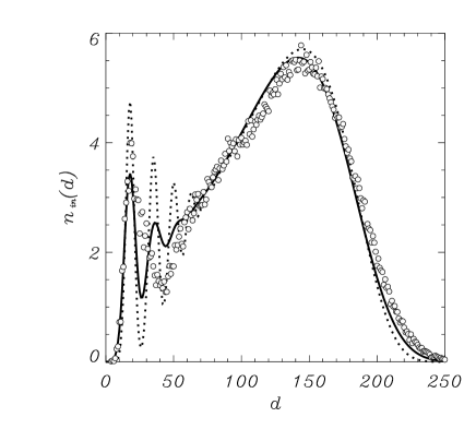
Figure 4: Comparison of the theoretical in-degree distributions with numerical data (circles). The dotted line shows the theoretical result for a network in the large $L$-limit, where the network is self-averaging and thus almost all possible realisations of a string of a given length $l$ can be found. The solid line is obtained after correcting for finite size effects (see text for details).

Unfortunately, we have not been able to obtain closed-form expressions for $d_{{\rm in},l}$ and $\tilde{\sigma}_{{\rm in},l}$, in a manner analogous to the expressions for the out-degree, Eqs. (53) and (69). In the case of the in-degree distributions, Eq. (88) requires a sum over the first argument of the matching probability, $p(\cdot,\cdot;z)$, Eq. (36), rather than the second argument, as was the case for the out-degree distribution. Due to the complicated dependence of the matching probability on its first argument this sum is, as far as we can tell, intractable. The necessary summations were therefore carried out numerically.

Figure (4) shows a comparison of the two theoretical predictions, Eqs. (91) and (92) with the numerical data of Balcan and Erzan Balcan-Erzan .

The in-degree distribution Eq. (91), and its finite-size corrected form, Eq. (92), capture the qualitative features seen in the simulations. Although there are deviations for small and large values of $d$, we will not pursue this any further in the present paper.

Note however the stark difference between the shape of the in- and out-degree distributions, Figs. (3) and (4). Apart from the distinct qualitative features, such as oscillatory behavior for small $d$ (rather than large $d$ as in the out-degree distribution), the in-degree distribution is much narrower than the out-degree distribution.

V Discussion

We have obtained analytical expressions for the in- and out-degree distribution of a contents-based network model which was introduced and studied numerically by Balcan and Erzan in Balcan-Erzan . We have shown that the behavior of the out-degree distribution can be divided into two regimes: a short and putative scaling regime for small out-degrees that crosses over into an oscillatory regime for large out-degrees. An analytical expression for the cross-over point has been obtained as well. We have found that the behavior of the out-degree distribution for large out degrees depends on the size of the network realizations from which the distribution was sampled. We have discussed these finite-size effects and have shown analytically how they effect the behavior of the out-degree-distribution.

Our results were obtained for a generalized class of contents-based network models in which a small number of imperfect matches (finite, but low, temperature) were allowed and strings were constructed from an alphabet of $r$ letters. It turns out, however, that such generalization do not alter the main numerical findings of the network model of Balcan and Erzan which involved a two-letter ($r=2$) alphabet and perfect matches. The scaling behavior which we have found, and even the numerical values of the leading scaling exponents $\gamma_{2}$ and $\gamma_{1}=\gamma_{2}+0.5$ are robust under these generalisations. It should be noted that, in

$$\gamma_{2}=\frac{1}{2}\frac{\ln z-\ln q}{\ln z+\ln q}\;\;,$$ (94)

we have $z\to 1/r$ for $\beta\to\infty$, while $z\to 1$ in the “high temperature” limit $\beta\to 0$, thus $r^{-1}\leq z\leq 1$. In the “low temperature,” or perfect matching, limit $\beta\to\infty$,

$$\gamma_{2}\to(1/2)(1-p/\ln r),$$ (95)

where $p$ is a small number by assumption Balcan-Erzan . Even when allowing for a small number of mismatches, $\gamma_{2}$ depends very weakly on $r$, and $p$. On the other hand, for either $r\to 1$, the trivial limit where no information is coded, or the high temperature limit, where no matching conditions are satisfied, the scaling relation is altered qualitatively, with $\gamma_{2}\to-1/2$.

We should remark on the robustness of the incipient power law behavior found in the limit of small degrees, for the out-degree distribution. Two different sources of randomness determine together the degree distributions of our model through the variables $d_{l}$ and $n_{l}$. While $d_{l}$ is determined by the adjacency rule based on sequence matching, and therefore depends on the length of the sequence to be matched, the distribution of nodes of length $l$ could have been chosen in many different ways. The exponential dependence turns out to be algebraically tractable, but it may be conjectured that any distribution which has a tail that is decaying exponentially with $l$ would give rise, all else remaining equal, to essentially the same scaling behavior for the out-degree distribution in the large $l$ (small $d$) regime, and therefore that $\gamma_{1}\simeq 1$ has a high degree of universality.

We would like to end this paper by pointing out the possible relevance of this network model to understanding molecular networks Mirni , in particular transcriptional genomic networks.

Transcriptional genomic networks are obtained by identifying the nodes with genes, and the directed edges connecting two nodes with so called transcription factors (TF). A TF is the protein coded by the gene at the node of origin, and binds (i.e., becomes chemically attached to) a short DNA sequence within the promoter region typically upstream of the target gene, whose activity it controls by either promoting, or suppressing it. genenetworks , biobook2

An assay of the recently available results coming from high-throughput experiments on the degree distribution of transcriptional genomic networks reveals that the out-degree distribution shows putative scaling over a very short range of about one decade at most, with a lot of scatter, and a marked departure from linearity on double logarithmic plots, for larger degrees. Nevertheless, with the assumption that $n(d)\sim d^{-\gamma}$ over the whole range, the exponents $\gamma$ which have been reported are all smaller than two, and closer to unity: $\gamma=1.4$ (yeast) Lee , $\gamma=1$ (yeast) Guelzim , $\gamma=1.1$-$1.8$ (several genomes) Barkai , $\gamma=1.5$ (E. coli) Dobrin , $\gamma=1.3$ (yeast) Tong .

Comparing these findings for the degree distribution of the transcriptional regulatory network with the results of our model is very suggestive. The marked but short range over which the data can indeed be fitted by a straight line in a log-log plot of the degree distribution has a power close to unity, as found in the experiments on transcriptional regulatory networks cited above. The crossover to a different regime towards the tail end of the distribution, is a feature that also shows similarity with the experimental results. Clearly the oscillations of the out-degree distribution, Figs. (1) and (3) are not seen in the degree distributions of the transcription regulatory networks extracted from any particular genome. In the language of our paper, real cellular networks are more like single finite-size realizations, rather than expected distributions calculated over ensembles of many different realizations of a random sequence. In our model, for any particular finite-size realization, only a relatively small number of data points would fall into this portion of the distribution and this would not be sufficient to resolve well the oscillations that make up the sample-averaged distribution. The small degree behavior of the degree distribution, however, is robust with respect to sample-to-sample fluctuations, as we have shown.

We think that the similarity with reported degree statistics of transcriptional genomic networks is not fortuitous. Sequence matching provides a highly plausible mechanism for the formation of the transcriptional regulatory network. Such networks rely on the recognition of regulatory sequences by transcription factors. These points will be discussed in detail within a more comprehensive comparison of features of content-based network models with real biological data in a forthcoming article Alkan .

Acknowledgements

One of us (AE) gratefully acknowledges partial support from the Turkish Academy of Sciences. MM gratefully acknowledges partial support from the Nahide and Mustafa Saydan Foundation. AK acknowledges support of FIRB01.

APPENDIX

Here we outline the calculations leading to Eqs. (22) and (26). In Section III, we defined the function $W^{(2)}(a,b;{\bf x})$ as, Eq. (19),

$$W^{(2)}(a,b;{\bf x})=\frac{1}{r^{k}}\sum_{{\bf y}}f_{a}({\bf x},{\bf y};\beta)f_{b}({\bf x},{\bf y};\beta)$$ (96)

As we pointed out in the text, when performing the sum over ${\bf y}$, two cases must be distinguished: (i) $|b-a|\geq l$ and (ii) $|b-a|<l$. In case (i), the set of indices of ${\bf y}_{a,l}$ and ${\bf y}_{b,l}$ are distinct and the evaluation of the partition sum proceeds in a manner analogous to Eq. (20) yielding

$$W^{(2)}(a,b;{\bf x})=\left(\frac{1}{r^{l}}\right)^{2}\left[1+(r-1)e^{-\beta}\right]^{2l},\,|b-a|\geq l.$$ (97)

In case (ii) there is an overlap between the indices of ${\bf y}_{a,l}$ and ${\bf y}_{b,l}$. Defining $|b-a|=m$, we find that there are $l-m$ overlapping indices, and thus there are $k-(l+m)$ distinct variables $y_{c}$ that are neither in ${\bf y}_{a,l}$ nor in ${\bf y}_{b,l}$, so that a sum over the values of these indices will give $r^{k-(l+m)}$. Next, it is convenient to partition the remaining indices, $\{y_{a+1},\ldots,y_{b+l}\}$, into the three disjoint sets, $S_{1}=\{y_{a+1},\ldots,y_{a+m}\}$, $S_{2}=\{y_{a+m+1}=y_{b+1},\ldots,y_{a+l}=y_{b+l-m+1}\}$ and $S_{3}=\{y_{b+a-m+2},\ldots,y_{b+l}\}$. Figure (5) shows an example for $l=7$, with $a=2$ and $b=5$ along with the sets, $S_{1}=\{y_{3},y_{4},y_{5}\}$, $S_{2}=\{y_{6},y_{7},y_{8},y_{9}\}$ and $S_{3}=\{y_{10},y_{11},y_{12}\}$. With the definitions above, we find for $|b-a|<l$,

$$W {}^{(2)}(a,b;{\bf x})=\frac{1}{r^{l+m}}\sum_{S_{1}}e^{-\beta\sum_{t=1}^{k}u(x_{t},y_{a+t})}$$

$$\times \sum_{S_{3}}e^{-\beta\sum_{t=1}^{m}u(x_{b+l-m+t}),y_{b+l-m+t})}$$

$$\times \sum_{S_{2}}e^{-\beta\sum_{t=1}^{l-m}\left[u(x_{t},y_{b+t})+u(x_{m+t},y_{b+t})\right]}$$

and carrying out the sums over the $y$ variables, we obtain ( $|b-a|<l$),

$$W^{(2)}(a,b;{\bf x})=\frac{1}{r^{l+m}}\left[1+(r-1)e^{-\beta}\right]^{2m}$$

$$\times\prod_{t=1}^{l-m}\left[1+(r-1)e^{-2\beta}-u(x_{t},x_{t+m})\left(1-e^{-\beta}\right)^{2}\right].$$ (99)

Figure 5: Schematic representation of the $y$ and $x$ averages for the function $W^{(2)}(a,b;\beta)$ as defined in the text. The case shown in the figure corresponds to $l=7$ with $a=2$ and $b=5$. The number of overlapping indices in the figure is $l-m(=4)$, with $m=b-a(=3)$. Because of the overlapping, when averaging over ${\bf x}$, these indices fall into $m(=3)$ disjoint sets: $\{x_{1},x_{4},x_{7}\}$, $\{x_{2},x_{5}\}$ and $\{x_{3},x_{6}\}$

.

Next, it is useful to introduce the $r\times r$ matrix, $M(x,y)$ as

$$M(x,y)=1+(r-1)e^{-2\beta}-u(x,y)\left(1-e^{-\beta}\right)^{2},$$ (100)

with $x,y\in\{0,1,2,\ldots,r-1\}$. From the properties of $u$, Eq. (8), we find that

$$M(x,y)=\left\{\begin{array}[]{ll}1+(r-1)e^{-2\beta},&x=y\\ (r-2)e^{-2\beta}+2e^{-\beta},&x\neq y\end{array}\right.$$ (101)

and Eq. (99) can therefore be written as

$$W^{(2)}(a,b;{\bf x}) = \frac{1}{r^{l+m}}\left[1+(r-1)e^{-\beta}\right]^{2m}$$ (102)

$$\times \prod_{t=1}^{l-m}M(x_{t},x_{t+m}).$$

Proceeding to perform the average over ${\bf x}$,

$$W^{(2)}(a,b)=\frac{1}{r^{l}}\sum_{{\bf x}}W^{(2)}(a,b;{\bf x}),$$ (103)

observe that in eq. (102) the variables ${\bf x}$ can be partitioned into $k$ disjoints sets $X$ with the additional property that if $x_{t}\in X$, by implication $x_{t+m}\in X$. The situation is shown schematically in Fig. (5) for $m=3$, where we have the $3$ disjoint sets, $\{x_{1},x_{4},x_{7}\}$, $\{x_{2},x_{5}\}$ and $\{x_{3},x_{6}\}$. Denoting these sets as $X_{1},X_{2},\ldots X_{m}$, and their respective number of elements as $n_{1},n_{2},\ldots,n_{m}$ ($n_{1}+n_{2}+\ldots n_{m}=l$), we see that the product in Eq.(102) can be factorized as

$$\prod_{t=1}^{l-m}M(x_{t},x_{t+m})=\prod_{x_{t}\in X_{1}}M(x_{t},x_{t+m})\cdots\prod_{x_{t}\in X_{m}}M(x_{t},x_{t+m})$$ (104)

Performing the summation over each of the factors we have for the first factor

$$\sum_{X_{1}}\prod_{x_{t}\in X_{1}}M(x_{t},x_{t+m}).$$ (105)

It can be easily shown that the sum over the variables $x_{t}\in X_{1}$ reduces to an $n_{1}-1$ fold matrix product. Denoting the matrix elements of the matrix $M^{n}$ by ${(M^{n})}_{xy}$, we therefore find

$$\sum_{X_{1}}\prod_{x_{t}\in X_{1}}M(x_{t},x_{t+m})=\sum_{x,y}{(M^{n_{1}-1})}_{xy}$$ (106)

and hence

$$\frac{1}{r^{l}}\sum_{\bf x}\prod_{t=1}^{l-m}M(x_{t},x_{t+m})=\frac{1}{r^{l}}\prod_{s=1}^{m}\sum_{x,y}{(M^{n_{s}-1})}_{xy}$$ (107)

Owing to the structure of the matrix $M$, Eq. (101), powers of $M$ retain the same structure, as can be readily shown, and we therefore have

$${(M^{n})}_{(xy)}=\left\{\begin{array}[]{ll}A_{n},&x=y\\ B_{n},&x\neq y.\end{array}\right.$$ (108)

The quantities $A_{n}$ and $B_{n}$ can be evaluated recursively, and one finds after a little algebra,

$$\left(\begin{array}[]{l}A_{n+1}\\ B_{n+1}\end{array}\right)=Q_{n}\left(\begin{array}[]{l}A_{1}\\ B_{1}\end{array}\right),$$ (109)

where

$$Q_{n}=\frac{1}{r}\left(\begin{array}[]{cc}(r-1)\lambda_{+}^{n}+\lambda_{-}^{n}&-(r-1)\lambda_{+}^{n}+(r-1)\lambda_{-}^{n}\\ -\lambda_{+}^{n}+\lambda_{-}^{n}&\lambda_{+}^{n}+(r-1)\lambda_{-}^{n}\end{array}\right),$$ (110)

and

$$\lambda_{+} = \left[1-e^{-\beta}\right]^{2}$$ (111)

$$\lambda_{-} = \left[1+(r-1)e^{-\beta}\right]^{2}.$$ (112)

We therefore find,

$$\sum_{x,y}{(M^{n})}_{xy}=rA_{n}+r(r-1)B_{n},$$ (113)

and thus

$$\sum_{x,y}{(M^{n})}_{xy}=r\left[1+(r-1)e^{-\beta}\right]^{2n}.$$ (114)

Substituting eq. (114) back into eq. (107) we have

$$\frac{1}{r^{l}}\sum_{\bf x}\prod_{t=1}^{l-m}M(x_{t},x_{t+m})=\frac{1}{r^{l}}\prod_{s=1}^{m}r\left[1+(r-1)e^{-\beta}\right]^{2(n_{s}-1)}$$ (115)

and noting that $n_{1}+n_{2}+\ldots n_{m}=l$, we finally obtain

$$\frac{1}{r^{l}}\sum_{\bf x}\prod_{t=1}^{l-m}M(x_{t},x_{t+m})=\frac{1}{r^{l}}r^{m}\left[1+(r-1)e^{-\beta}\right]^{2(l-m)},$$ (116)

which when substituted into Eqs. (103) and (102) yields the final result, Eq. (23),

$$\frac{1}{r^{l}}\sum_{{\bf x}}W^{(2)}(a,b;{\bf x})=\frac{1}{r^{2l}}\left[1+(r-1)e^{-\beta}\right]^{2l}.$$ (117)

Note that we obtain the same result as for the case $|b-a|>l$, Eq. (97). In particular, we see that once averaged over ${\bf x}$, $W^{(2)}$ is independent of $a$ and $b$.

References

- [1] D. Balcan and A. Erzan, Eur. Phys. J. B 38, 253 (2004).
- [2] R. Pastor-Satorras and A. Vespignani, Evolution and Structure of the Internet- A statistical physics approach(Cambridge University Press, Cambridge, 2004)
- [3] P. Erdös and A. Renyi, Publ. Mat. (Debrecen) 6, 290 (1959); Publ. Mat. Inst. Hung. Acad. Sci. 5, 17 (1960) and Bull. Inst. Int. Stat. 38, 343 (1961), cited in R. Albert and A.-L. Barabasi, Rev. Mod. Phys. 74 47 (2002).
- [4] A.-L. Barabasi and R. Albert, Science 286 509 (1999).
- [5] R. Albert and A.-L. Barabasi, Rev. Mod. Phys. 74 47 (2002).
- [6] S. Özçelik and A. Erzan, Int. Jour. Mod. Phys. C, 14(2003) 169.
- [7] G. E. Uhlenbeck and G. W. Ford, Lectures in Statistical Mechanics (American Mathematical Society, Providence, 1963); K. Huang Statistical Mechanics (John Wiley and Sons. N.Y., 1987).
- [8] S. Altschul, W. Gish, W. Miller, E.W. Meyers, and D. Lipman, J. Mol. Biol. 225, 403 (1990).
- [9] S. Karlin and S. F. Altschul, Proc. Natl. Acad. Sci. 87,2264 (1990).
- [10] S. Karlin and S. F. Altschul, Proc. Natl. Acad. Sci. 90, 5673 (1993).
- [11] W. Feller, An Introduction to Probability Theory and its Applications, (Wiley, N.Y. 1971).
- [12] V. Spirin and L.A. Mirny, Proc. Nat. Acad. Sci. 100, 12123 (2003).
- [13] R. V. Sole and R. Pastor-Satorras, “Complex Networks in Genomics and Proteomics,” S. Bornholdt and H.G.Schuster eds., Handbook of Graphs and Networks (Wiley-VCH Verlag, Berlin 2002).
- [14] B. Alberts et al., Molecular Biology of the Cell (Garland Science, N.Y., 2002), Chapter 9.
- [15] T.I. Lee et al., Science 298, 799 (2002).
- [16] N. Guelzim, S. Bottani, P. Bourgine, F. Kepes, Nature Genetics 31, 61 (2002).
- [17] S. Bergmann, J. Ihmels, N. Barkai, PloS Biology, 2,0085 (2004). http://biology.plosjournals.org (2003).
- [18] R. Dobrin, Q.K. Beg, A.-L. Barabasi and Z.N. Oltvai, BMC Bioinformatics 5, 1 (2004).
- [19] A. Hin Yan Tong et al., Science 303, 808 (2004).
- [20] A.Kabakçıoğlu, M. Mungan, D. Balcan, A. Erzan, in preparation.