Amino acid substitution matrices for protein conformation identification

Abstract

Methods for alignment of protein sequences typically measure similarity by using substitution matrix with scores for all possible exchanges of one amino acid with another. Although widely used, the matrices derived from homologous sequence segments, such as Dayhoff’s PAM matrices and Henikoff’s BLOSUM matrices, are not specific for protein conformation identification. Using a different approach, we got many amino acid segment blocks. For each of them, the protein secondary structure is identical. Based on these blocks, we have derived new amino acid substitution matrices. The application of these matrices led to marked improvements in conformation segment search and homologues detection in twilight zone.

PACS number(s): 87.10.+e,02.50.-r

1 Introduction

The similarity of amino acids is the basis of protein sequence alignment, protein design, and protein structure prediction.The mutation data matrices of Dayhoff[1] and the substitution matrices of Henikoff[2] are standard choices of scores for amino acid similarity evaluation. Although, widely used in protein design and protein structure prediction, these matrices pay more attention to homologous relationship than to conformation similarity.

However, in studies of protein conformations, the task is to detect whether residue sequences have similar conformations neglecting their homologous relationships. Several works[3, 4] showed that residue behavior is influenced by protein conformations. Therefore, we wondered whether a better approach might be to use alignments in which these relationships are explicitly represented.

For this purpose, we derived many residue segment blocks from the nonredundant PDB_SELECT[5] database. The amino acid segments in each of the block have identical protein secondary structure according to the database of secondary structure in proteins(DSSP)[6]. Consequently, based on the counts of residue substitution in our database, we derived the amino acid substitution matrices for protein conformation identification.

2 Methods

We created a nonredundant set of 1612 non-membrane proteins from PDB_SELECT with amino acid identity less than 25% issued on 25 September of 2001. The secondary structure for these sequences were taken from DSSP database. In DSSP algorithm, Kabsch and Sander defined eight states of secondary structure according to the hydrogen-bond pattern. As in most methods, we considered 3 states $\{h,e,c\}$ generated from the 8 by the coarse-graining $H,G,I\to h$, $E\to e$ and $X,T,S,B\to c$.

2.1 Constructing blocks databases

For this work, we constructed blocks database from our dataset by the following two rules:

(1) Each amino acid segment in a block has the same protein secondary structure;

(2) Each amino acid segment in a block has at least one non-gapped high scored alignment when it is compared with other segments in the block.

Step 1: A window of width $l$ is sliding along every sequence of our dataset. A dataset $G$ of amino acid segments $a_{0}a_{1}...a_{l-1}$ with the corresponding secondary structure segments $s_{0}s_{1}...s_{l-1}$ is created. For an entry $a^{j}_{0}a^{j}_{1}...a^{j}_{l-1}$ in dataset $G$, if there is another entry $a^{k}_{0}a^{k}_{1}...a^{k}_{l-1}$ in $G$ which satisfies $s^{j}_{0}=s^{k}_{0},s^{j}_{1}=s^{k}_{1},...s^{j}_{l-1}=s^{k}_{l-1}$ and $S\geq S_{0}$

$$S=\sum^{i=l-1}_{i=0}score(a^{j}_{i},a^{k}_{i});$$ (1)

then the entry is added to dataset $B^{\prime}_{s_{0}s_{1}...s_{l-1}}$, where $score(a^{j}_{i},a^{k}_{i})$ is the score for residues $a^{j}_{i},a^{k}_{i}$ substitution in BLOSUM62[2] matrix. After filtering set $\{B^{\prime}\}$ to forbid sample recounts in the original dataset, we get some high scored residue segments for different protein secondary structure words.

Step 2: To reduce the contributions to amino acid pair frequencies from the less similar residue segments, segments of each protein secondary structure word in set $\{B^{\prime}\}$ are clustered. This is done by specifying the threshold $S_{0}$, identical to that used in step 1 , in which segments that have alignment score $S$ better than $S_{0}$ are grouped together. For example, in dataset $B^{\prime}_{s_{0}s_{1}...s_{l-1}}$, if the score $S_{XY}\geq S_{0}$ when segments $X$ and $Y$ are aligned, then $X$ and $Y$ are clustered. If segment $Z$ has a high scored alignment with either $X$ or $Y$, it is also clustered with them.

After these two steps, we get a new blocks database fulfilling our requirements.

2.2 Deriving amino acid substitution matrices
from conformational blocks databases

To reduce multiple contributions to amino acid pair frequencies from the most closely related members in a block, sequences are clustered within blocks and each cluster is weighted as a single sequence in counting pairs. This is done by specifying a clustering percentage in which sequence segments that are identical for at least that percentage of amino acids are grouped together. In our work, we adjust this percentage to that of the original BLOSUM matrices are derived.

We count all possible pairs of amino acid substitution in each column of every block. All these counts are summed. The result of this counting is a frequency table listing the number of times each of the $20+19+..1=210$ different amino acid pairs occurs among the blocks. The table is used to calculate a matrix representing the odds ratio between these observed frequencies and those expected by chance.

We denote the total number of amino acid $i,j$ pairs($1\leq j\leq i\leq 20$) by $f_{ij}$. Then the observed probability of occurrence for each $i,j$ pair is

$$q_{ij}=f_{ij}/\sum_{i=1}^{20}\sum_{j=1}^{i}f_{ij}$$ (2)

The probability for the amino acid $i$ to occur is then

$$p_{i}=q_{ii}+\sum_{j\neq i}q_{ij}/2$$ (3)

The expected probability of occurrence $e_{ij}$ for each $i,j$ pair is then $p_{i}p_{j}$ for $i=j$ and $p_{i}p_{j}+p_{j}p_{i}=2p_{i}p_{j}$ for $i\neq j$. An odds ratio matrix is calculated where each entry is $q_{ij}/e_{ij}$. A lod ratio is then calculated in bit units as $s_{ij}=\log_{2}(q_{ij}/e_{ij})$. Lod ratios are multiplied by a scaling factor of 2 and then rounded to the nearest integer value to produce CBSM(conformational blocks substitution matrix) matrices in half-bit units. For each substitution matrix, we calculated the average mutual information per amino acid pair $H$(also called relative entropy)[7], and the expected score $E$ in bit units as

$$H=\sum_{i=1}^{20}\sum_{j=1}^{i}q_{ij}\times s_{ij},\qquad E=\sum_{i=1}^{20}\sum_{j=1}^{20}p_{i}\times p_{j}\times s_{ij}.$$ (4)

For more details on matrix driving, we refer reader to Refs.[2]

2.3 Protein secondary structure segment searches

To evaluate the improvement of the performance of our amino acid substitution matrices to that of the original BLOSUM matrix used, we do a protein secondary structure segment search in the learning set. All-against-all segment alignment is carried out in dataset $G$. For two segments $X$ and $Y$, the alignment score $S_{XY}\geq T_{0}$, if they have the same protein secondary structure then there is a sample of Ture-Positive, else a False-Positive sample.

Given a threshold $T_{0B}$, using BLOSUM matrix, we get the counts of Ture-Positive and False-Positive samples in dataset $G$. As our substitution matrix is used, by varying the threshold $T_{0}$, we adjust the counts of False-Positive samples to that of the original BLOSUM matrix used. Consequently, we can evaluate the improvement by the counts of Ture-Positive samples.

2.4 Homologous pairs detection

To evaluate the validity of the above scheme, we examine whether the sequence alignments with CBSM60 perform better than those with BLOSUM62 for homologous sequences in the twilight zone. For this propose, we use the 176 sequences test set extracted by Elber et, al[8]. Each homologous pair in the test set have a sequence identity less than 25%, but very similar structure.

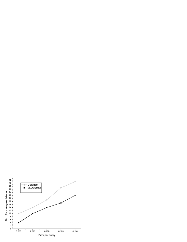
Figure 1: The number of successfully identified homologous pairs in the 176 sequences test set as a function of errors per query.

We perform all-against-all sequence alignment on the test set with Blast2.2.6[9, 10]. The gap insertion and elongation parameters used for alignment are set to 11/1. Detective ability is illustrated by the number of successfully identified homologous pairs as a function of errors per query. The error per query is defined as the total number of non-homologous protein sequences detected with expectation value equal to or less than the threshold divided by the total number of aligned sequence pairs. By varying the expectation value cutoff of Blast, we get the results shown in figure 1.

3 Result

By setting $S_{0}=27$, we created $l=10$ width blocks from our dtatset. The resulting amino acid substitution matrices are shown in table 1.

It is interesting to make a comparison between the CBSM60 matrices obtained here with the commonly used BLOSUM62 matrices. There are many remarkable differences between the two score schemes. Lots of amino acid pairs have more negative score in CBSM60 than those in BLOSUM matrices. For example, the scores for residue pairs CN, CD, ID, WD, QC, KC, FC, WK, and WP are more than two bits lesser than those in BLOSUM62 matrix. This means dissimilar residues are strongly forbidden in amino acid substitution. On the other hand, the scores for some pairs of similar residues are slightly improved, such as SA, SN, LI, VI, MI, ML, VL, FM, YF, and ST.

Relative entropy is 0 when the target(or observed) distribution of pair frequencies is same as the background(or expected) distribution and increases as these two distribution become more distinguishable. Based on relative entropy, the BLOSUM90 is comparable to CBSM60 with relative entropy of $\approx 1.2$ bit. Some differences are seen when BLOSUM90 is subtracted from CBSM60 for every matrix entries. Compared to CBSM60, self substitution is more preferable in BLOSUM90. For some amino acids, especially PW, WD, and QC, CBSM60 is less tolerant to mismatches than BLOSUM90 is . On the contrary, some substitutions, such as MA, FM, SN, VL, and VY, are more tolerable in CBSM60.

The results of protein secondary structure segment searches are shown in table 3. We find that there is a remarkable improvement compared with those using BLOSUM matrix. The Ture-Positive sample count for each $T_{0B}$ increases nearly 15%. For False-positive cases, the proportion of samples with tiny structural differences between two aligned segments increases nearly one percent. This means the CBSM substitution matrices work very well.

In the results of homologous pairs detection shown in figure 1, we find that, compared with BLOSUM62, CBSM60 performs better. The detected homologues increase nearly 1/3. Further more, for cases where signal of sequence similarity is larger, we do the homologues detection too. Compared with BLOSUM62, for SCOP40 database[11, 12] where only PDB sequences that have 40% homology or less are included, there is a slightly increase($\approx$2%) with CBSM60 for homologues detection.

Since the residues in each column of a block correspond to an uniform secondary structure, we can get the residue pair counts and calculate the amino acid substitution matrix for different protein conformation states. The results are shown in table 4-6. When the three matrices are compared with each other, we find many differences. For example, comparing helix with sheet , the similarities of CA, SR, MQ, PH, and TP change drastically. There is a positive score for Cysteine and Alanine substitution in helix. While in sheet conformation, the score is negative.

4 Discussions

We have found that substitution matrices based on amino acid pairs in conformational blocks of aligned protein segments perform better in protein secondary structure segment identification and homologues detection than those based on Henikoff’s BLOSUM score scheme. Because the CBSM matrices can also be used in three dimensional structure identification(This part will be published elsewhere. ), the importance of such improved performance can be profound for works in protein design and protein conformation prediction.

Furthermore, CBSM is indeed a different scheme from BLOSUM. For example, in the performance of homologues detection by CBSM60, we found that 6 of 10 detected homologous pairs are different from those detected using BLOSUM62 as the error per query equals 0.05. When the error per query is 0.15, this portion is 19 of 31. This means a new score scheme have been provided which can detect a different scope of remote homologous relationship from Henikoff’s BLOSUM matrices.

There are fundamental differences between our approach and that of Henikoff that could account for the superior performance of CBSM matrices. In their case,based on Prosite database, blocks were derived primarily from the most highly conserved regions of proteins in residue sequence means neglecting the conformation identity. Many of the differences between CBSM and BLOSUM matrices may arise from multi-conformation regions of conserved sequence.

Our results show the strong dependence of residue behavior on conformations. From table 4-6, we find that there are many residue pairs displaying strong dependence of similarity on conformations. We expect that specially derived scores for multiple conformations should work better in researches of protein structure. This will be discussed elsewhere.

This work is part of the project 10347145 supported by National Natural Science Foundation of China.

Table 1. CBSM60 substitution matrix(Lower) and difference matrix(Upper) obtained by subtracting the BLOSUM62 matrix position by position.

    A   R   N   D   C   Q   E   G   H   I   L   K   M   F   P   S   T   W   Y   V
    1   0  -1  -1  -1   0  -1  -1   0  -1   0   0   1   0  -1   1   0  -3   0   0  A
        1   0  -1  -2   0   0  -1   0  -1  -1   0   0   0  -1   0   0  -3  -1  -1  R
A   5       0   0  -4   0  -1   0   0  -2  -1   0  -3  -1  -2   1   0  -2  -2  -2  N
R  -1   6       0  -5   0   0  -1  -1  -4  -3  -1  -2  -2  -2   0  -1  -6  -3  -3  D
N  -3   0   6       0  -5  -3  -1  -2  -1  -1  -4  -1  -4  -2  -2  -1  -3  -2  -2  C
D  -3  -3   1   6       0   0  -1   0  -1   0   0  -1  -3  -3   0   0  -3  -1  -2  Q
C  -1  -5  -7  -8   9      -1  -2   0  -2  -2   0  -1  -3  -2   0  -1  -2  -2  -2  E
Q  -1   1   0   0  -8   5       1  -2  -3  -1  -1  -1  -2   0   0  -1  -2  -2  -1  G
E  -2   0  -1   2  -7   2   4       0  -2   0   0  -1  -1  -2   0  -1  -3  -1  -1  H
G  -1  -3   0  -2  -4  -3  -4   7       0   1  -1   1   0  -3  -1   0  -2  -1   1  I
H  -2   0   1  -2  -5   0   0  -4   8       0  -1   1   0  -3  -1   0   0  -1   1  L
I  -2  -4  -5  -7  -2  -4  -5  -7  -5   4       0  -1  -1  -2   0   0  -4  -1  -1  K
L  -1  -3  -4  -7  -2  -2  -5  -5  -3   3   4       0   1  -2   0  -1  -1   0   0  M
K  -1   2   0  -2  -7   1   1  -3  -1  -4  -3   5       1   0  -1  -1  -1   1   0  F
M   0  -1  -5  -5  -2  -1  -3  -4  -3   2   3  -2   5       0  -1  -1  -7  -3  -2  P
F  -2  -3  -4  -5  -6  -6  -6  -5  -2   0   0  -4   1   7       0   1   0  -1  -2  S
P  -2  -3  -4  -3  -5  -4  -3  -2  -4  -6  -6  -3  -4  -4   7       1  -2  -1   0  T
S   2  -1   2   0  -3   0   0   0  -1  -3  -3   0  -1  -3  -2   4      -1  -1  -3  W
T   0  -1   0  -2  -2  -1  -2  -3  -3  -1  -1  -1  -2  -3  -2   2   6       0   0  Y
W  -6  -6  -6 -10  -5  -5  -5  -4  -5  -5  -2  -7  -2   0 -11  -3  -4  10       0  V
Y  -2  -3  -4  -6  -4  -2  -4  -5   1  -2  -2  -3  -1   4  -6  -3  -3   1   7
V   0  -4  -5  -6  -3  -4  -4  -4  -4   4   2  -3   1  -1  -4  -4   0  -6  -1   4
    A   R   N   D   C   Q   E   G   H   I   L   K   M   F   P   S   T   W   Y   V

Table 2. The difference matrix between CBSM60 and BLOSUM90 obtained by subtracting the BLOSUM90 matrix position by position.

A   0
R   1   0
N  -1   1  -1
D   0   0   0  -1
C   0   0  -3  -3   0
Q   0   0   0   1  -4  -2
E  -1   1   0   1  -1   0  -2
G  -1   0   1   0   0   0  -1   1
H   0   0   1   0   0  -1   1  -1   0
I   0   0  -1  -2   0   0  -1  -2  -1  -1
L   1   0   0  -2   0   1  -1   0   1   2  -1
K   0   0   0  -1  -3   0   1  -1   0   0   0  -1
M   2   1  -2  -1   0  -1   0   0   0   1   1   0  -2
F   1   1   0   0  -3  -2  -1   0   0   1   0   0   2   0
P  -1   0  -1   0  -1  -2  -1   1  -1  -2  -2  -1  -1   0  -1
S   1   0   2   1  -1   1   1   1   1   0   0   1   1   0   0  -1
T   0   1   0   0   0   0  -1   0  -1   0   1   0  -1   0   0   1   0
W  -2  -2  -1  -4  -1  -2   0   0  -2  -1   1  -2   0   0  -6   1   0  -1
Y   1   0  -1  -2   0   1   0   0   0   0   0   0   1   1  -2   0  -1  -1  -1
V   1  -1  -1  -1  -1  -1  -1   1   0   1   2   0   1   1  -1  -2   1  -3   2  -1
    A   R   N   D   C   Q   E   G   H   I   L   K   M   F   P   S   T   W   Y   V

Table 3. Results of protein secondary structure segment searches.
Protein secondary structure differences 0 1 2 3 4 5 6 7 8 9 10 $T_{0B}$ ($T_{P}$) Percentage of $F_{p}$ $F_{p}$ CBSM60 101745 7.8 9.2 10.5 11.0 11.3 11.3 10.7 9.7 7.7 10.7 1368517 23 BLOSUM62 86601 6.9 8.7 10.5 11.4 12.0 12.0 11.3 9.9 7.6 9.7 1389714 CBSM60 46999 8.1 9.5 10.8 11.1 11.4 11.3 10.6 9.5 7.5 10.2 597618 25 BLOSUM62 39522 7.2 9.0 10.8 11.6 12.1 12.0 11.1 9.7 7.3 9.2 588929 CBSM60 20612 8.5 9.9 11.0 11.3 11.5 11.3 10.5 9.3 7.2 9.6 242292 27 BLOSUM62 17841 7.6 9.3 11.0 11.8 12.2 12.0 10.9 9.5 7.0 8.6 243169 CBSM60 9272 8.9 10.3 11.2 11.4 11.5 11.3 10.3 9.0 6.9 9.1 98926 29 BLOSUM62 8175 8.1 9.7 11.3 11.8 12.4 12.0 10.6 9.1 6.8 8.1 98219 CBSM60 4356 9.7 10.7 11.4 11.6 11.6 11.2 9.9 8.7 6.7 8.5 39101 31 BLOSUM62 3942 8.9 10.2 11.5 11.9 12.5 11.9 10.1 9.0 6.7 7.4 38688

Table 4. Amino acid substitution matrix CBSM60c for coil state(Lower) and difference matrix(Upper) obtained by subtracting the CBSM60h matrix position by position. The bold entries are pairs which have different positive/negative signs in the two compared matrices.
A R N D C Q E G H I L K M F P S T W Y V -1 1 -1 -1 -3 0 2 0 1 1 2 2 1 0 1 0 0 2 2 1 A 1 0 0 1 1 0 -1 -2 2 2 1 1 4 -3 1 0 1 4 3 R A 4 -2 0 1 0 -1 -2 0 3 1 -1 2 2 -2 0 -1 7 0 3 N R 0 6 -1 2 -1 0 -2 0 1 1 0 1 5 1 -1 -1 4 0 -1 D N -3 0 5 -3 -4 2 2 -4 1 0 -1 -1 -5 -6 -4 -2 7 -3 -3 C D -3 -3 1 5 1 1 -2 0 2 3 1 3 5 1 0 1 -1 3 3 Q C -2 -4 -7 -8 8 1 -1 0 4 2 1 3 4 2 0 1 1 1 3 E Q -1 2 0 -1 -11 5 -4 -3 -1 -1 0 2 1 1 -2 -3 1 -1 1 G E 0 0 -1 2 -6 3 5 1 -1 1 1 4 0 2 -1 0 4 1 4 H G 0 -3 -1 -3 -5 -3 -3 5 2 1 0 1 0 2 2 2 4 1 1 I H -1 -2 1 -2 -7 0 0 -5 9 1 1 1 1 1 1 0 -2 0 1 L I -1 -2 -3 -6 0 -3 -2 -6 -6 5 0 2 1 1 0 1 1 3 1 K L 0 -1 -3 -6 -1 0 -4 -5 -3 4 5 1 1 -3 1 3 -3 0 1 M K 0 3 -1 -2 -8 2 1 -3 -1 -4 -2 5 1 3 2 0 3 1 1 F M 0 0 -3 -4 -2 1 -1 -2 -1 3 4 0 6 -6 0 -1 -3 4 3 P F -3 -1 -3 -3 -8 -3 -3 -4 -2 0 1 -3 1 8 0 0 3 2 2 S P -1 -4 -5 -3 -7 -3 -2 -4 -4 -5 -4 -2 -4 -3 5 -1 2 1 1 T S 2 0 1 -1 -5 0 0 -1 -2 -1 -2 0 0 -2 -3 4 1 0 4 W T 0 -1 0 -2 -3 0 -1 -4 -3 0 -1 -1 0 -4 -3 2 5 1 -1 Y W -5 -5 -3 -7 -3 -7 -4 -3 -4 -2 -4 -6 -5 2 -11 -2 -2 11 1 V Y -1 -1 -4 -5 -5 0 -3 -5 2 -1 -2 -1 -1 5 -5 -2 -2 1 8 V 1 -2 -3 -6 -4 -2 -2 -3 -2 5 3 -2 2 0 -2 -2 0 -2 -2 5 A R N D C Q E G H I L K M F P S T W Y V

Table 5. Amino acid substitution matrix CBSM60e for sheet state(Lower) and difference matrix(Upper) obtained by subtracting the CBSM60c matrix position by position. The bold entries are pairs which have different positive/negative signs in the two compared matrices.
A R N D C Q E G H I L K M F P S T W Y V 1 -1 2 0 -1 1 -1 1 0 -1 -1 -1 0 1 -4 0 0 -1 -3 -1 A 0 1 1 0 1 2 0 2 -3 -3 0 -1 -2 3 1 0 -2 -1 -1 R A 5 3 -1 2 2 2 2 -1 -6 -1 2 -1 -4 2 2 0 -3 1 -3 N R -1 6 4 2 2 0 1 1 -1 -1 1 -1 -5 -1 2 -3 1 -3 0 D N -1 1 8 2 8 -1 -2 2 -4 -2 3 -2 0 4 -1 0 -1 -3 1 C D -3 -2 0 9 1 0 2 1 0 -4 0 1 -3 0 0 -1 5 -3 -2 Q C -3 -4 -5 -6 10 1 2 0 -2 -3 1 -5 -3 2 0 1 -1 -2 -2 E Q 0 3 2 1 -3 6 3 -3 0 0 0 -3 -1 0 2 0 -4 0 0 G E -1 2 1 2 -7 3 6 -1 3 1 0 -3 -1 5 2 2 1 -1 -2 H G 1 -3 1 -2 -7 -1 -1 8 -3 -2 0 -2 -2 2 -2 -2 -6 -3 -3 I H -1 0 0 -1 -5 1 0 -8 8 -1 -2 -1 -1 -3 -1 -1 2 0 -2 L I -2 -5 -9 -7 -4 -3 -4 -6 -3 2 1 -2 -1 -3 1 0 -2 -4 -2 K L -1 -4 -4 -7 -3 -4 -7 -5 -2 2 4 -1 -1 2 -1 -2 0 -2 -1 M K -1 3 1 -1 -5 2 2 -3 -1 -4 -4 6 -2 -2 0 2 -3 -2 -2 F M 0 -1 -4 -5 -4 2 -6 -5 -4 1 3 -2 5 6 1 4 7 -1 -6 P F -2 -3 -7 -8 -8 -6 -6 -5 -3 -2 0 -4 0 6 1 0 -5 0 -4 S P -5 -1 -3 -4 -3 -3 0 -4 1 -3 -7 -5 -2 -5 11 0 -3 -2 -1 T S 2 1 3 1 -6 0 0 1 0 -3 -3 1 -1 -2 -2 5 -2 -1 -9 W T 0 -1 0 -5 -3 -1 0 -4 -1 -2 -2 -1 -2 -2 1 2 5 -2 -1 Y W -6 -7 -6 -6 -4 -2 -5 -7 -3 -8 -2 -8 -5 -1 -4 -7 -5 9 -2 V Y -4 -2 -3 -8 -8 -3 -5 -5 1 -4 -2 -5 -3 3 -6 -2 -4 0 6 V 0 -3 -6 -6 -3 -4 -4 -3 -4 2 1 -4 1 -2 -8 -6 -1 -11 -3 3 A R N D C Q E G H I L K M F P S T W Y V

Table 6. Amino acid substitution matrix CBSM60h for helix state(Lower) and difference matrix(Upper) obtained by subtracting the CBSM60e matrix position by position. The bold entries are pairs which have different positive/negative signs in the two compared matrices.
A R N D C Q E G H I L K M F P S T W Y V 0 0 -1 1 4 -1 -1 -1 -1 0 -1 -1 -1 -1 3 0 0 -1 1 0 A -1 -1 -1 -1 -2 -2 1 0 1 1 -1 0 -2 0 -2 0 1 -3 -2 R A 5 -1 1 -3 -2 -1 0 1 3 0 -1 -1 2 0 -2 1 -4 -1 0 N R -1 5 -3 -4 -1 0 1 -1 0 0 -1 0 0 0 -1 4 -5 3 1 D N -2 0 7 1 -4 -1 0 2 3 2 -2 3 5 2 5 2 -6 6 2 C D -2 -3 1 6 -2 -1 0 -1 -2 1 -1 -4 -2 -1 0 0 -4 0 -1 Q C 1 -5 -8 -10 11 -2 -1 0 -2 1 -2 2 -1 -4 0 -2 0 1 -1 E Q -1 1 0 0 -7 4 1 6 1 1 0 1 0 -1 0 3 3 1 -1 G E -2 0 0 2 -8 2 4 0 -2 -2 -1 -1 1 -7 -1 -2 -5 0 -2 H G 0 -2 1 -1 -7 -1 -2 9 1 1 0 1 2 -4 0 0 2 2 2 I H -2 0 1 -2 -3 0 0 -2 8 0 1 0 0 2 0 1 0 0 1 L I -2 -4 -6 -7 -1 -5 -6 -5 -5 3 -1 0 0 2 -1 -1 1 1 1 K L -2 -3 -4 -7 -1 -3 -6 -4 -4 3 4 0 0 1 0 -1 3 2 0 M K -2 2 0 -2 -7 1 0 -3 -2 -4 -3 5 1 -1 -2 -2 0 1 1 F M -1 -1 -5 -5 -1 -2 -4 -4 -5 2 3 -2 5 0 -1 -3 -4 -3 3 P F -3 -5 -5 -8 -3 -8 -7 -5 -2 0 0 -4 0 7 -1 0 2 -2 2 S P -2 -1 -3 -4 -1 -4 -4 -5 -6 -7 -5 -3 -1 -6 11 1 1 1 0 T S 2 -1 1 0 -1 0 0 1 -1 -3 -3 0 -1 -4 -3 4 1 1 5 W T 0 -1 1 -1 -1 -1 -2 -1 -3 -2 -1 -2 -3 -4 -2 2 6 1 2 Y W -7 -6 -10 -11 -10 -6 -5 -4 -8 -6 -2 -7 -2 -1 -8 -5 -4 10 1 V Y -3 -5 -4 -5 -2 -3 -4 -4 1 -2 -2 -4 -1 4 -9 -4 -3 1 7 V 0 -5 -6 -5 -1 -5 -5 -4 -6 4 2 -3 1 -1 -5 -4 -1 -6 -1 4 A R N D C Q E G H I L K M F P S T W Y V

References

- [1] M. O. Dayhoff and R. V. Eck. Atlas of Protein Sequence and Structure (Natl. Biolmed. Res. Found.Silver Springs, MD). 3, 33(1968).
- [2] S. Henikoff and J.G. Henikoff. Proc. Natl. Acad. Sci. 89, 10915(1992).
- [3] J.U. Bowie, R. Lüthy, and D. Eisenberg. Science 253, 164(1991).
- [4] X.Liu, L.M.Zhang, S.Guan, and W.M.Zheng. Physical Review E 67, 051927(2003).
- [5] U.Hobohm and C.Sander,Protein Science 3,522(1994).
- [6] W.Kabsch and C.Sander,Biopolymers 22, 2577(1983).
- [7] R.E.Blahut. Principles and Practice of Information Theory(Addison-Wesley, Reading, MA). (1987)
- [8] O. Teodorescu, T. Galor, J. Pillardy, and R. Elber, Proteins: Struct. Funct. Bioinform 54, 41(2004).
- [9] S.F. Altschul, T.L. Madden, A.A. Schäffer, J. Zhang, Z. Zhang, W. Miller, and D.J. Lipman, Nucleic Acids Res., 25, 3389 (1997).
- [10] S.F. Altschul, J. Mol. Biol., 219, 555 (1991).
- [11] S.E. Brenner, C. Chothia, and J.P. Hubbard, Proc. Natl. Acad. Sci. (USA), 95, 6073 (1998).
- [12] A.G. Murzin, S.E. Brenner, T. Hubbard, and C. Chothia, J. Mol. Biol., 247, 536 (1995).