Finite Width Model Sequence Comparison

Abstract

Sequence comparison is a widely used computational technique in modern molecular biology. In spite of the frequent use of sequence comparisons the important problem of assigning statistical significance to a given degree of similarity is still outstanding. Analytical approaches to filling this gap usually make use of an approximation that neglects certain correlations in the disorder underlying the sequence comparison algorithm. Here, we use the longest common subsequence problem, a prototype sequence comparison problem, to analytically establish that this approximation does make a difference to certain sequence comparison statistics. In the course of establishing this difference we develop a method that can systematically deal with these disorder correlations.

I Introduction

Sequence comparison gathers interest from a wide variety of fields such as molecular biology, biophysics, mathematics, and computer science. Methods of comparison concern computer scientists who use string comparison for everything from file searches to image processing Paterson ; danc94a ; danc94b ; wate94 . Biological sequence comparison provides details into the building blocks of life by allowing the functional identification of newly found sequences through similarity to already studied ones. Thus, it has become a standard tool of modern molecular biology.

As with all pattern search algorithms, a crucial component for the successful application of sequence comparisons is the ability to discern the biologically meaningful from randomly occurring patterns. Thus, a thorough characterization of the strength of patterns within random data is mandatory to establishing a criterion for discerning meaningful data karl90 .

The most commonly used sequence alignment algorithms are the closely related Needleman-Wunsch need70 and Smith-Waterman smit81 algorithms. There have been numerous numerical and analytical studies that attempt to characterize the behavior of these algorithms on random sequence data wate94a ; wate94b ; alts96 ; olse99 ; mott99 ; mott00 ; sieg00 ; bund02 ; metz02 . However, there are difficulties with both kinds of approaches to the problem of characterizing sequence alignment algorithms statistically. The numerical methods are by far too slow to be useful in an environment where tens of thousands of searches are performed on a daily basis and users expect their results on interactive time scales. The analytical methods on the other hand, while in principle able to rapidly characterize sequence alignment statistics, are only valid in small regions of the vast parameter space of the sequence alignment algorithms.

In addition to being restricted to a small region of parameter space, current analytical methods have another drawback: they rely on an approximation to the actual alignment algorithm that ignores some subtle correlations within the sequence disorder. Here, we want to demonstrate that such correlations do matter and propose an analytical approach that can in principle deal with these correlations for certain finite size variants of sequence alignment introduced in section III.

We will concentrate on the simplest prototype of a sequence alignment algorithm, namely the longest common subsequence (LCS) problem. More complicated models of sequence alignment can be adapted to the methodology presented here in a straightforward manner. However, in the interest of clarity and efficiency, we proceed with the simple LCS problem in mind. In the longest common subsequence problem similarity between two randomly chosen sequences over an alphabet of size $c$ is measured by the length of the longest string that can be constructed from both sequences solely by deleting letters. The central quantity characterizing the statistics of the LCS problem is the expected length of this longest common subsequence. Its fraction of the total sequence length in the limit of infinitely long sequences is called the Chvátal-Sankoff constant $a_{c}$.

Although the LCS problem is one of the simplest alignment algorithms, the value of the Chvátal-Sankoff constant has been remarkably elusive. So far, analytical stabs at $a_{c}$ have led to exact solutions for very short lengths chva75 and proofs for upper and lower bounds Paterson ; chva75 ; hirs78 ; chva83 ; deke83 ; danc94a ; danc94b ; alex94 . Based on numerical results, there existed a long-standing conjecture for the value of the Chvátal-Sankoff constant. Recently demo99 ; bund00 , this conjecture has been proven to hold true for the approximation to the LCS problem that precisely ignores the disorder correlations mentioned above. Very careful and extensive numerical treatments danc94a ; danc94b ; demo99 ; demo00 ; bund01 ; dras01 have revealed that the true Chvátal-Sankoff constant (including all disorder correlations) deviates slightly from its value in the uncorrelated approximation. This paper seeks to introduce a systematic way of understanding the LCS problem with all disorder correlations included and to establish in an analytically tractable environment that uncorrelated and correlated disorder indeed lead to different results.

The format of this paper will be to summarize the LCS problem in section II. This section includes a general description of the LCS problem and outlines a commonly used paradigm for solving for the LCS. In addition, several conventions which are utilized throughout the paper are defined here. In section III we introduce the finite width model (FWM) method. In order to spare the reader possibly distracting mathematical details we discuss only the overall ideas in the main text and reserve appendix A for the more detailed discussion of the mathematical methods employed in FWM. In section IV we give the results of the FWM method for the correlated and uncorrelated LCS problem and discuss the differences between these two problems that become obvious in the FWM treatment. Section V summarizes our findings.

II Review of the LCS problem

The LCS of two sequences is the longest sequence that can be formed solely by deletions in both sequences chva75 . Best described by example, the LCS of ’DARLING’ and ’AIRLINE’ is ’ARLIN’, with a subsequence length of 5. Given two sequences of length $M$ and $N$, $x_{1}x_{2}...x_{M}$ and $y_{1}y_{2}...y_{N}$, over an alphabet of size c, their LCS can be computed in $O(MN)$ time. This computation may be conveniently visualized with a rectangular grid such as the one shown in Fig. 1. In this example, for the two sequences, $x_{1}x_{2}...x_{6}$ = ’001001’ and $y_{1}y_{2}...y_{6}$ = ’010110’, the LCS, ’0100’, has a length of 4. Within the grid used to find the LCS, all horizontal and vertical bonds are assigned a value of 0. Each diagonal bond is designated a value depending on the associated letters in its row and column. Matching letters earn their diagonal bonds a value of 1, while non-matching letters result in an assignation of 0. Then, each directed path across these various bonds from the first lattice point in the upper-left to the last in the lower-right as drawn in Fig. 1 corresponds to a common subsequence of the two sequences. The only restriction is that the path may never proceed against the order of the sequences. It may only move rightward, downward, or right-downward in Fig. 1. The length of a common subsequence corresponding to a path is the sum of the bonds which comprise that path. Solving this visual game for the length of the LCS requires that we find the path of greatest value. This value will be the length of the LCS.

Recursively, we may define this problem by introducing the quantity $\ell(i,j)$ as the LCS of the substrings $x_{1}x_{2}...x_{i}$ and $y_{1}y_{2}...y_{j}$. Defining the LCS of two substrings in this way allows us to find the LCS leading to each of the lattice points in Fig. 1. This in turn breaks our path search down into the more manageable steps.

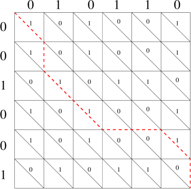
Figure 1: Grid representation of the longest common subsequence (LCS) problem. The dashed line highlights a solution to the LCS of the two binary sequences on the edges of the square. Notice that there exist multiple solutions to this problem.

$$\ell(i,j)=\max\left\{\begin{array}[]{l}\ell(i-1,j)\\ \ell(i-1,j-1)+\eta(x,y)\\ \ell(i,j-1)\end{array}\right\}$$ (4)

where

$$\eta(i,j)=\left\{\begin{array}[]{ll}1&x_{i}=y_{j}\\ 0&\mbox{otherwise}\end{array}\right.$$ (7)

and

$$\ell(0,j)=\ell(i,0)=0.$$ (8)

Of course, once we evaluate the final $k(M,N)$, we have solved for the length of the LCS. Ultimately, we wish to evaluate the central quantity that characterizes the LCS problem, the Chvátal-Sankoff constant $a_{c}$. It characterizes the ensemble of LCS’s of pairs of randomly chosen sequences with $M=N$ independently identically distributed (iid) letters. If we denote averages over the ensemble by $\langle...\rangle_{N}$, the Chvátal-Sankoff constant may be defined as

$$a_{c}\equiv\underset{N\rightarrow\infty}{\lim}\frac{\langle LCS\rangle_{N}}{N}$$ (9)

This can be interpreted as the average growth rate of the LCS of two random sequences.

As evident from Fig. 1 and the recursive equations (4)-(8) the length of the LCS depends on the sequences only via the values of the $\eta$’s. If we define the probabilities of 0 or 1 occurring in our random sequences as $p$ or $1-p$, respectively, where $0\leq p\leq 1$, each individual $\eta$ carries a $2(1-p)p$ probability of being zero, and a $p^{2}+(1-p)^{2}$ of being 1. However, the different $\eta(i,j)$ are not chosen independently according to those probabilities, but are subject to subtle correlations.

It is very tempting to neglect these correlations in favor of choosing $N^{2}$ iid variables $\widehat{\eta}(i,j)$ according to

$$\widehat{\eta}(i,j)=\left\{\begin{array}[]{lll}1&\mbox{with probability}&1-q\\ 0&\mbox{with probability}&q\end{array}\right.$$ (12)

where $q=2(1-p)p$, the probability of a bond value being 0. We will call this the uncorrelated LCS problem and identify all quantities calculated for this problem by an additional hat; specifically, we will call $\widehat{a}_{c}$ the analog of the Chvátal-Sankoff constant in the uncorrelated LCS problem. This approximation to the real LCS problem has been used in various theoretical approaches to sequence comparison statistics mott99 ; demo99 ; bund02 . For the LCS problem itself, only very careful numerical studies could show that the Chvátal-Sankoff constant for the correlated and uncorrelated problem are actually different danc94a ; danc94b ; demo99 ; demo00 . However, there are very real differences. The differences arise due to the fact that the correlated and uncorrelated cases allow different sets of possible bond or $\eta$ values. In the uncorrelated case all combinations of bond values are allowed to exist. The grid in Fig. 1 makes it obvious that there are $NM$ bonds each with 2 possibilities. Therefore, there must exist $2^{NM}$ unique configurations of bond values. Meager by comparison are the $2^{M+N-1}$ cases allowed by the two sequences of length M and N, with each letter having the capacity to take on one of two values in the correlated case. Notice the missing factor of 2 in the correlated case arises due to the fact that one can alway replace all 0’s with 1’s in order to get the same sequences of matches cutting our possible number of bond value configurations in half. A more concrete realization of the limited possibilities in the correlated case comes simply by noticing that there are only two bond value configurations values any row or column can take up in Fig. 1. Additionally, a column or row with a value of 0 must be a mirror opposite of a column or row with a value of 1. And so we can see that not only does the uncorrelated case account for sets of bond values that cannot exist, it cannot mimic the specific relationship between different rows and columns of bond values. We will reveal these differences in a simple approximation to the LCS problem that allows for closed analytical solutions in the correlated and uncorrelated case.

III Finite Width LCS

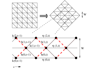
Figure 2: This picture shows our $45^{o}$ counter-clockwise rotation to achieve the orientation from which we will proceed. The blow up defines the lattice site values (k-values), the match values ($\eta$-values), and the lattice site difference values (h-values). It also defines our time and width axes. The dashed lines connect the sites between which our h-values are measured.

The Finite Width Model (FWM) we will use in the following overlays the grid presented in Fig. 1 with the restriction in width presented in Fig. 2 bund00 ; bund01 . We will measure the width $W$ of such a grid by the number of bands that make up the lattice, i.e. $W=2$ in Fig. 2. Although, the grid used to analyze the LCS must be truncated to a finite width W, our finite strip extends to an infinite length. Thus, we can still define a width dependent Chvátal-Sankoff constant

$$a_{c}(W)=\underset{N\rightarrow\infty}{\lim}\frac{\langle\ell(N,N)\rangle_{N}}{N}$$ (13)

In addition to the width $W$, the growth rate also depends on the sequence composition. In our case of alphabet size $c=2$ this is characterized by the probability $p$ to find a ’0’ on each site within the sequences. While the method we will present below in principle enables us to calculate any $a_{c}(W,p)$, we will, in the following, concentrate on the simple example $a_{c}(W=2,p)$ shown in Fig. 2. Notice that

$$a_{c}=\underset{W\rightarrow\infty}{\lim}a_{c}(W,\frac{1}{2})$$ (14)

from below, and thus $a_{c}(W,\frac{1}{2})$ produces a series of lower bounds to the Chvátal-Sankoff constant.

On the finite width lattice shown in Fig. 2, it is convenient to redefine our quantities. Aside from the narrower scope under which we investigate the LCS problem, all other properties of the grid problem remain the same. Instead of referring to our lattice points by the coordinates $i$ and $j$, we now utilize a time axis, $t$, which points along the allowed, sequence forward, direction as well as a coordinate axis, $x$, which lies perpendicular to the $t$-axis. In place of old $\ell$-values, in this new coordinate system we introduce $k$-values. Keeping track of these $k$-values can be simplified to a new set of recursive relationships at each time step. In the notation defined by Fig. 2 for width $W=2$,

$$k(2,t+1)=\max\left\{\begin{array}[]{l}k(2,t)+\eta(2,t)\\ k(1,t)\end{array}\right\}$$ (17)

$$k(1,t+1)=\max\left\{\begin{array}[]{l}k(2,t+1)\\ k(1,t)+\eta(1,t)\\ k(0,t+1)\end{array}\right\}$$ (21)

$$k(0,t+1)=\max\left\{\begin{array}[]{l}k(1,t)\\ k(0,t)+\eta(0,t)\end{array}\right\}$$ (24)

where the $\eta$’s take on values of either 1 or 0 in the same way that we assigned values to our diagonal lines in Fig. 1. Our set of recursive relationships gives us the longest path value up to each lattice site. The length of the FWM LCS then becomes $k(1,N)$.

Related to our $k$-values by equations (25) and (26), we define the $h$-values in order to describe the relative values of our lattice sites within any given time frame. Utilizing the diagrammed definitions of Fig. 2,

$$h(1,t)=k(1,t)-k(2,t)$$ (25)

$$h(0,t)=k(1,t)-k(0,t).$$ (26)

The recursion relations (17),(21) and (24), can be expressed entirely via this new quantity as

$$h(1,t+1)=\max\left\{\begin{array}[]{l}0\\ h(1,t)+\eta(1,t)-r(1,t)\\ h(1,t)+s(0,t)-r(1,t)\end{array}\right\}$$ (30)

$$h(0,t+1)=\max\left\{\begin{array}[]{l}0\\ h(0,t)+\eta(0,t)-r(0,t)\\ h(0,t)+s(1,t)-r(0,t)\end{array}\right\}$$ (34)

where

$$r(1,t) = \max\left\{\eta(2,t),h(1,t)\right\}$$ (35)

$$r(0,t) = \max\left\{\eta(0,t),h(0,t)\right\}$$ (36)

$$s(1,t) = \max\left\{0,\eta(2,t)-h(1,t)\right\}$$ (37)

$$s(0,t) = \max\left\{0,\eta(0,t)-h(0,t)\right\}$$ (38)

Several properties conveniently arise from these definitions. First, notice that the $h$-values are independent of the absolute $k$-values. Furthermore, it may be shown by inspection that the $h$-values may only take on the values $(0,1)$. Inspecting Fig. 2, we note that each adjacent set of $k$-values share a nodal $k$. This node attaches itself to the adjacent sites via a bond of value 0 or 1. Since the nodal $k$ holds only a single value and the single bonds leading to the adjacent sites can only change this value by +1, the only $h$-values allowed then become 0 or 1. Having detached the absolute $k$-values from the FWM-LCS problem entirely, we may further detach the entire FWM from the grid in Fig. 1. Originally we noted that our FWM-LCS on this grid becomes $k(1,N)$. However, in order to calculate $a_{c}(W,p)$, the length of the LCS problem has to be increased infinitely along the time axis. Time now becomes an unbounded axis in the FWM. Since the difference $|k(x,t)-k(y,t)|$ is bounded by $W$ for all $x$ and $y$, the length of the LCS may be measured at any $x$. The growth rate may then be expressed as the average $k$-values increase along any coordinate, i.e.

$$a_{c}(W,p)=\langle k(x,t)-k(x,t-1)\rangle$$ (39)

Notice that $k(x,t)-k(x,t-1)\epsilon\left\{0,1\right\}$ and that as a result our newly defined $a_{c}(W,p)$ carries the condition $0\leq a_{c}(W,p)\leq 1$.

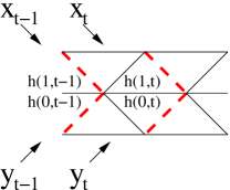
Figure 3: The diagram maps the influence of letters from the two sequences …, $x_{t-1}$, $x_{t}$, … and …, $y_{t-1}$, $y_{t}$, … on the new orientation. The letter information required for the evolution from time $t-1$ to time $t$ is shown here. The dashed lines represent the chosen configuration for the $h$’s.

The formulation given by equations (30), (34) make it clear that $h(1,t)$ and $h(0,t)$ can be calculated if $h(1,t-1),h(0,t-1),\eta(2,t-1),\eta(1,t-1)$, and $\eta(0,t-1)$ are known. This allows us to write the time evolution as a Markov model. In order to do so, the information required for the time evolution at each time step must be included in the states. For our uncorrelated states, where the $\eta$’s occur randomly, only $h(1,t-1)$ and $h(0,t-1)$ are required to determine the probable time evolution. Therefore, the uncorrelated states simply read ($h(1,t-1)$, $h(0,t-1)$). The probabilities for the time evolution into the state ($h(1,t)$, $h(0,t)$) may then be calculated based on the $\eta$-value probabilities given in equation (7). However, in the correlated case, the $\eta$’s are not randomly chosen. Instead, the letters in each sequence are according to the probability $p$ of a 0 occurring at a single site within the sequences. Some letters affect $\eta$’s across multiple time steps as shown by Fig. 3. In order to calculate the time evolution to time $t$, $\eta(2,t-1),\eta(1,t-1)$, and $\eta(0,t-1)$ must be known. These $\eta$’s depend on the subsequences $x_{t-1},x_{t}$ and $y_{t-1},y_{t}$. Once these four letters are known, the state at time $t$ may be determined. Since these letters cast an influence across multiple time steps, their information must be retained in order to accurately forecast the upcoming possibilities for the $\eta$’s and our states. Redefining our states as ($h(1,t),h(0,t),x_{t},y_{t}$) preserves the necessary information. The remaining information for calculating the $\eta$’s needed for the time evolution, mainly $x_{t+1}$ and $y_{t+1}$, arise according to the letter probabilities. These probabilities contribute to the probable time evolution into the next $t+1$ state ($h(1,t+1),h(0,t+1),x_{t+1},y_{t+1}$). It can be shown that correlated states must always contain $W$ $h$-values and $W$ letter values, and that uncorrelated states must always contain $W$ $h$-values.

Though the number of elements in a state depends only on the width, there exist alternative means of writing our states. We are free to choose whatever configuration of continuous lines to define our $h$-values across. Fig. 4 show the other possible configurations in width 2 FWM. Naturally, the letter effects differ for each shape, and the proper letters for each configuration are also illustrated. The various states we may form all contain the same number of $h$ and letter values and obey the same principles. Only the specified set of $h$ and letter values differ.

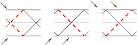
Figure 4: The dashed lines represent the various configurations by which the $h$-values can be defined. Note that each of the various sets of $h$-values implies a different definition of the state, and thus requires a different set of letters. The arrows represent the letters which are required in each different configuration.

Whatever state we choose to define, the Markov process  describing FWM-LCS is characterized by a transfer matrix $\hat{T}$. This matrix describes the transitions from a state in one time to a state in it’s immediate future. It is a representation of the dynamics given by Eqs. (30)-(38). We leave the mechanics of obtaining this transfer matrix to Appendix A and focus here on the results.

Once we have found the transfer matrix we may solve for the vector ${\vec{s}}$ describing the steady state by solving the linear system of eigenvalue equations

$${\hat{T}}\cdot{\vec{s}}={\vec{s}}$$ (40)

subject to the normalization condition ${\vec{1}}\cdot{\vec{s}}=1$ where ${\vec{1}}=(1,1,1,1,...)$. Note that the size of these vectors depends on the number of states needed to describe the problem. More specifically, 16 elements are needed for the correlated width 2 FWM while the uncorrelated width 2 case only requires 4 elements. This steady state vector must contain the probabilities to observe every single state in the random ensemble. Note that the directness of this technique allows for it’s ready adaptation to more complex sequence comparison algorithms along the lines of Ref. bund02 . However, this generally requires a significantly larger number of states thus incurring a greater computational cost.

In order to describe the growth rate, we utilize a growth matrix $\hat{G}$ to mark the transitions which result in growth along some chosen coordinate. The process by which we construct the growth matrix bears great similarity to the process by which we construct the transfer matrix. In fact, the growth matrix only omits those elements of the transfer matrix that do not contribute to the growth along a chosen coordinate. Further detail regarding the construction of the growth matrix has been left for Appendix A.

The growth matrix allows us to define the growth vector, ${\vec{g}}$

$${\vec{g}}={\vec{1}}\cdot{\hat{G}}$$ (41)

This growth vector describes the probable growth from each of the states. Coupled with the steady state, which provides us with the likelihood of each state, this allows us to solve for $a_{c}(W,p)$ directly as

$$a_{c}(W,p)={\vec{g}}\cdot{\vec{s}}$$ (42)

since the probability of growth from $t\rightarrow t+1$, as described by the growth matrix, is independent of the probability to be in a certain state at time $t$.

Before we discuss the results of this approach, we would like to point out that this technique is not limited to the calculation of the growth rate $a_{c}(W,p)$. Since the dynamics of the scores is a Markov process, any quantity can be calculated once the transfer matrix $\hat{T}$ and the steady state vector $\vec{s}$ are known. E.g., any equal-time correlation function of interest can be obtained directly from the steady-state vector $\vec{s}$ simply by summing over the degrees of freedom that are not to be included in the correlation function while a time-correlation function like $\langle i(t)|j(t^{\prime})\rangle$ (the probability to be in state $i$ at time $t$ given that the system was in state $j$ at time $t^{\prime}$) is simply given by $\langle i(t)|j(t^{\prime})\rangle=\vec{i}\cdot\hat{T}^{t-t^{\prime}}\vec{j}$ where $\vec{i}$ and $\vec{j}$ are vectors, all entries of which are zero except for a one in the row for state $i$ or $j$, respectively.

Solving the correlated width $W=2$ FWM-LCS problem utilizing the process given by equations (40)-(42), we arrive at the equation

$$a_{2}(W=2,p)=\frac{3-5p+5p^{2}}{3-p-3p^{2}+8p^{3}-4p^{4}}$$ (43)

where $p$ represents the probability of the first letter occurring. The same methodology may be applied to the uncorrelated case, where we describe the transition probabilities using the bond probability q defined by equation (12).

$$\widehat{a}_{2}(2,q)=\frac{5-7q+2q^{2}}{5-5q+q^{2}}$$ (44)

Notice that the specifics of the state that we choose does not impact the result in any way. Nor does the choice we make with respect to measuring the growth. Any combination of choices result in equations (43) and (44) for the correlated and uncorrelated cases respectively. We explicitly verified this independence in the choice of configurations and definitions of the growth. These independent results serve as a powerful check for the correctness of the algebraic manipulations. Substituting $q=2(1-p)p$ into equation (45), the probability of getting two different letters, or a bond value of 0, gives a an equation expressed in the same quantities as the correlated Chvátal-Sankoff constant given by equation (43), mainly

$$\widehat{a}_{2}(2,p)=\frac{5-14p+22p^{2}-16p^{3}+8p^{4}}{5-10p+14p^{2}-8p^{3}+4p^{4}}$$ (45)

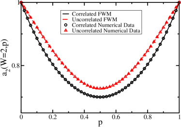
Figure 5: Analytical and numerical data provided by FWM. This plot shows further evidence verifying the correctness of FWM. Numerical modeling obtained by passing many random sequences through an FWM evaluation produces the data points represented. The analytical FWM model matches the numerical data with high precision for both the correlated and uncorrelated cases at width $W=2$. The error for the numerical data presented is smaller than the symbol size.

IV Results

Now, we will apply our method to various small width cases and discuss the implications of the results for the longest common subsequence problem. First, we check our computations, and plot the results Eqs. (43) and (45) alongside numerical data obtained by random sampling in Fig. 5. The numerical data obtained by choosing $10,000$ pairs of random sequences of length $10,000$, calculating their width $2$ LCS and averaging shows no discernable deviation from the analytical results over the whole range of the parameter $p$. Already in this plot for $W=2$, the differences between the correlated and uncorrelated cases are apparent. Coinciding only for $p=0$ and $p=1$ where growth is certain in every step, the two cases differ at all other points.

width $W$	correlated case	uncorrelated case
0	$\frac{1}{2}$ (0.5)	$\frac{1}{2}$ (0.5)
1	$\frac{2}{3}\ (0.\bar{6})$	$\frac{2}{3}\ (0.\bar{6})$
2	$\frac{7}{10}$ (0.7)	$\frac{8}{11}\ (0.\bar{72})$
3	$\frac{1592}{2201}$ (0.723307587)	$\frac{34}{45}\ (0.7\bar{5})$
4	$\frac{3900482569}{5288762638}$ (0.737503808)	$\frac{152}{197}$ (0.771573604)
5	$\frac{1016932681760084189805278879341973703014985562}{1359136362951380586870384955918322158719785917}$ (0.748219759)	$\frac{706}{903}$ (0.781838317)
$\infty$	(0.8126)	(0.828427125)

Table 1: Finite-width Chvátal-Sankoff constant $a_{2}(W,\frac{1}{2})$ for correlated and $\widehat{a}_{2}(W,\frac{1}{2})$ for uncorrelated disorder. As a reference the value of the Chvátal-Sankoff constant for infinite width is given. In the correlated case it is only known numerically bund01 ; in the uncorrelated case it is given by $2/(\sqrt{2}+1)$ demo99 ; bund00 .

Then, we look at the width dependence of the growth rates at the symmetric point $p=1/2$. They are summarized in Table 1. The results again verify the difference between the correlated and uncorrelated cases with the growth rate in the uncorrelated case being systematically higher than in the correlated case. They also highlight two rather interesting exceptions. The first occurs for the case $W=0$ in which correlations play no role and indeed have no meaning. Assigning a random bond value (uncorrelated) or two random letters (correlated) lead to the same effect. Thus, as expected, the correlated and uncorrelated cases plot identically for $W=0$. The second exception, occurring for $W=1$, narrows the scope of equality to three values of $p$, namely $0,\frac{1}{2},$ and $1$. In these cases, the equality arises from the exactly similar bond values being produced from each case. In all other respects, the correlated and uncorrelated versions of $W=1$ differ.

Viewing the solutions of Table 1 also shows that the growth rate $a_{c}$ increases with width $W$. This agrees with perfectly with the expectations of the FWM. As width increases so do the possibilities for growth. In fact, in the limit $W\rightarrow\infty$ we recover the Chvátal-Sankoff constant - the infinite width growth rate. Along the way, these finite width values of $a_{c}$ provide lower bounds to the Chvátal-Sankoff constant. In this way, FWM conveniently provides a method for gathering systematic solutions for obtaining lower bounds to the Chvátal-Sankoff constant. The values given for $a_{c}$ in this table may be read as a series of ever increasing analytically solved lower bounds. In this systematics, FWM displays one of it’s advantages over conventional methods. However, the power and exactness of these solutions exacts a computational cost that grows as $2^{12W}$.

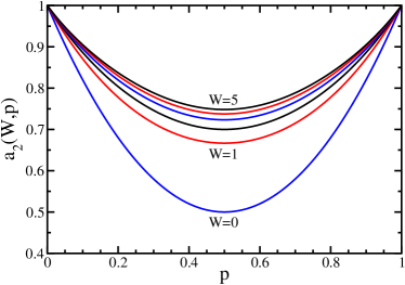
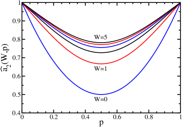
Figure 6: Finite width growth rates as a function of the letter probability $p$ for different widths.

Next, we consider the dependence of the growth rates on the letter probability $p$. Fig. 6 shows the full analytical solutions for various widths plotted as a function of $p$. These graphs verify the trend noted from the discussion of Table 1. However, they allow another interesting observation: while the difference in values in the correlated and uncorrelated cases may be immediately perceived, the shape of each of the curves appears to not depend on $W$. With increasing $W$ the curve simply appears to come closer and closer to one. In order to verify this, we rescale the difference $1-a_{c}(W,p)$ of the growth rate from one by its value $1-a_{c}(W,1/2)$ at $p=1/2$. As shown in Fig. 7 these rescaled curves are indeed indistinguishable for $W=2,3,4,$ and $5$. They clearly fall into two distinct classes, namely a curve for the correlated case and a curve for the uncorrelated case. For the uncorrelated case, where the result $\widehat{a}_{c}(W=\infty,p)=2/[(p^{2}+(1-p)^{2})^{-1/2}+1]$ for infinite width is known demo99 ; bund00 , Fig. 7 also shows perfect agreement between the finite $W$ and the infinite $W$ results. Thus, at least in the uncorrelated case there are no noticeable finite size effects in the scaling function even for widths as small as $W=2$. Assuming the absence of finite size effects even for small widths also holds true for the correlated case for which we cannot independently verify this assumption, the results shown in Fig. 7 support two important conclusions: (i) the correlated and uncorrelated systems truly and systematically differ for all widths and thus also in the limit $W\to\infty$, and (ii) these curve shapes can be understood as universal properties of the correlated and uncorrelated FWM-LCS system independent of the width $W$. It implies that, given the value of $a_{c}$ for any $p\not=0$ or $1$ one may plot $a_{c}$ for all values of p. In other words, a single data point suffices to define a finite width system whether it be correlated or uncorrelated.

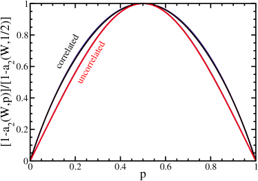
Figure 7: Rescaled growth rate for $W=2,3,4,5$ in the correlated and uncorrelated case as well as the $W=\infty$ result for the uncorrelated case. All results for the correlated case and all results of the uncorrelated case are virtually indistinguishable from each other while the correlated growth rate clearly follows a pattern that is distinctly different from the uncorrelated growth rate.

The differences between the correlated and uncorrelated case, highlighted by Fig. 7, result from the subtle restrictions that correlations place on bond values. As an example, for width 2 FWM, three bond values contribute to a single transition. Thus $2^{3}=8$ unique sets of bond values exist. Uncorrelated bond values allow for any of these $8$ possibilities at any given time. However, because the letters effect correlated bonds in multiple time steps, each correlated state has only $4$ allowed transitions. In fact, in any width the FWM provides a maximum of $4$ allowed transitions for all correlated states. The reasons for this are elucidated in Appendix A. In addition to the number of possibilities lacking in the correlated case, the allowed transitions create subtle relationships creating patterns of growth that differ significantly from the uncorrelated case. These differences account for the systematic separation viewed in Fig. 7.

V Conclusion

We conclude that within the FWM method differences between the correlated and uncorrelated LCS problem can be established analytically. The dependence of the finite width growth rate on the letter probability $p$ follows a scaling law already for the relatively small widths which are analytically accessible. These scaling laws are distinctively different for the correlated and uncorrelated case within FWM thereby providing an analytical argument that the differences between the correlated and uncorrelated case explicitly revealed for small finite widths here may persist in the limit of infinite widths. This is the first piece of analytical evidence that hints at the distinctness of the Chvátal-Sankoff constants in the correlated and uncorrelated cases. However, though there exists an analytical solution for the infinite width uncorrelated case, it should be noted that no such solution for the infinite width correlated case is available. Thus this evidence has only been analytically verified for widths up to 5 for correlated finite width systems, and the pattern suggested by this data set may yet be the result of some finite width effect. Nonetheless, the FWM method in itself provides a systematic means to deal with these correlations that can be generalized from the LCS to other sequence comparison problems.

Appendix A Obtaining the Transfer and Growth Matrices

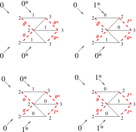
Figure 8: Above the four possible futures or transitions available to the state (0,0,0,0) are obtained diagrammatically. These transitions, reading from the upper left, are (0,0,0,0), (1,0,1,0), (0,1,0,1) and (1,1,1,1). Note that the states are organized with h values first, then letters both written in from the top to the bottom in this diagram. In order to help clarify the origin of these four sets of numbers, the quantities relevant to the new states have been starred.

Our transfer matrix, as discussed in the main text, describes transitions from one state into the next. It allows us to determine the probable fraction of time spent in any state, i.e. the steady state, and coupled with the growth matrix it allows us to calculated the growth rate. Obtaining the matrix elements involves finding all transition probabilities and placing them into our matrix. To begin, one simply takes a state and writes all possible transitions out of this state. When one has done this for all possible states, then the transfer matrix is complete. As an example we have calculated the first column of the transfer matrix in the correlated case $W=2$.

Starting with the first column, which represents our (0, 0, 0, 0) state, we note that there exist only four possible futures. Once we choose the two remaining letters as (0, 0), (1, 0), (0, 1) or (1, 1) the differences $h$ are completely determined. Fig. 8, shows the determination of the state transitions that result from these four sets of letters. These four transition then become the matrix elements of the first column. The probability weighing each transition is determined by the new set of letters that bring about the new state, or the starred letters in Fig. 8. In the order listed above, the states they bring about are weighed by the probabilities $p^{2}$, $(1-p)p$, $p(1-p)$, and $(1-p)^{2}$.

In order to formulate a growth matrix, we pick the line defining the growth, and delete the elements of the transfer matrix which do not contribute to the growth on this line. In this example we have chosen to measure our growth along the bottom line. As an example, in Fig. 8, the two top diagrams contribute to growth because the lattice value along the bottom line grows in both these cases. However, for the bottom pair, the lower lattice value remains static, thus their contributions are missing from the growth matrix shown below.

Repeating this for each possible starting state leads to the following matrix representations where the states are ordered from least to greatest in binary (0000, 0001, 0010, 0011,…).

$$\mbox{\large$\displaystyle{\hat{T}}=$}\left(\begin{array}[]{cccccccccccccccc}p^{2}&0&0&0&0&0&0&0&0&0&0&0&0&0&0&0\\[2.84526pt] 0&(1\!\!-\!\!p)p&(1\!\!-\!\!p)p&0&0&(1\!\!-\!\!p)p&0&(1\!\!-\!\!p)p&(1\!\!-\!\!p)p&(1\!\!-\!\!p)p&0&0&(1\!\!-\!\!p)p&(1\!\!-\!\!p)p&(1\!\!-\!\!p)p&(1\!\!-\!\!p)p\\[2.84526pt] 0&(1\!\!-\!\!p)p&(1\!\!-\!\!p)p&0&(1\!\!-\!\!p)p&0&(1\!\!-\!\!p)p&0&0&0&(1\!\!-\!\!p)p&(1\!\!-\!\!p)p&(1\!\!-\!\!p)p&(1\!\!-\!\!p)p&(1\!\!-\!\!p)p&(1\!\!-\!\!p)p\\[2.84526pt] 0&0&0&(1\!\!-\!\!p)^{2}&0&0&0&0&0&0&0&0&0&0&0&0\\[2.84526pt] 0&0&p^{2}&0&p^{2}&0&p^{2}&0&0&0&0&0&0&0&0&0\\[2.84526pt] (1\!\!-\!\!p)p&0&0&0&(1\!\!-\!\!p)p&0&(1\!\!-\!\!p)p&0&0&0&0&0&0&0&0&0\\[2.84526pt] 0&0&0&(1\!\!-\!\!p)p&0&(1\!\!-\!\!p)p&0&(1\!\!-\!\!p)p&0&0&0&0&0&0&0&0\\[2.84526pt] 0&(1\!\!-\!\!p)^{2}&0&0&0&(1\!\!-\!\!p)^{2}&0&(1\!\!-\!\!p)^{2}&0&0&0&0&0&0&0&0\\[2.84526pt] 0&p^{2}&0&0&0&0&0&0&p^{2}&p^{2}&0&0&0&0&0&0\\[2.84526pt] 0&0&0&(1\!\!-\!\!p)p&0&0&0&0&0&0&(1\!\!-\!\!p)p&(1\!\!-\!\!p)p&0&0&0&0\\[2.84526pt] (1\!\!-\!\!p)p&0&0&0&0&0&0&0&(1\!\!-\!\!p)p&(1\!\!-\!\!p)p&0&0&0&0&0&0\\[2.84526pt] 0&0&(1\!\!-\!\!p)^{2}&0&0&0&0&0&0&0&(1\!\!-\!\!p)^{2}&(1\!\!-\!\!p)^{2}&0&0&0&0\\[2.84526pt] 0&0&0&p^{2}&0&p^{2}&0&p^{2}&0&0&p^{2}&p^{2}&p^{2}&p^{2}&p^{2}&p^{2}\\[2.84526pt] 0&0&0&0&0&0&0&0&0&0&0&0&0&0&0&0\\[2.84526pt] 0&0&0&0&0&0&0&0&0&0&0&0&0&0&0&0\\[2.84526pt] (1\!\!-\!\!p)^{2}&0&0&0&(1\!\!-\!\!p)^{2}&0&(1\!\!-\!\!p)^{2}&0&(1\!\!-\!\!p)^{2}&(1\!\!-\!\!p)^{2}&0&0&(1\!\!-\!\!p)^{2}&(1\!\!-\!\!p)^{2}&(1\!\!-\!\!p)^{2}&(1\!\!-\!\!p)^{2}\end{array}\right)$$

$$\mbox{\large$\displaystyle{\hat{G}}=$}\left(\begin{array}[]{cccccccccccccccc}p^{2}&0&0&0&0&0&0&0&0&0&0&0&0&0&0&0\\[2.84526pt] 0&0&(1\!\!-\!\!p)p&0&0&(1\!\!-\!\!p)p&0&(1\!\!-\!\!p)p&0&0&0&0&(1\!\!-\!\!p)p&(1\!\!-\!\!p)p&(1\!\!-\!\!p)p&(1\!\!-\!\!p)p\\[2.84526pt] 0&(1\!\!-\!\!p)p&0&0&(1\!\!-\!\!p)p&0&(1\!\!-\!\!p)p&0&0&0&0&0&(1\!\!-\!\!p)p&(1\!\!-\!\!p)p&(1\!\!-\!\!p)p&(1\!\!-\!\!p)p\\[2.84526pt] 0&0&0&(1\!\!-\!\!p)^{2}&0&0&0&0&0&0&0&0&0&0&0&0\\[2.84526pt] 0&0&0&0&p^{2}&0&p^{2}&0&0&0&0&0&0&0&0&0\\[2.84526pt] 0&0&0&0&(1\!\!-\!\!p)p&0&(1\!\!-\!\!p)p&0&0&0&0&0&0&0&0&0\\[2.84526pt] 0&0&0&0&0&(1\!\!-\!\!p)p&0&(1\!\!-\!\!p)p&0&0&0&0&0&0&0&0\\[2.84526pt] 0&0&0&0&0&(1\!\!-\!\!p)^{2}&0&(1\!\!-\!\!p)^{2}&0&0&0&0&0&0&0&0\\[2.84526pt] 0&p^{2}&0&0&0&0&0&0&p^{2}&p^{2}&0&0&0&0&0&0\\[2.84526pt] 0&0&0&(1\!\!-\!\!p)p&0&0&0&0&0&0&(1\!\!-\!\!p)p&(1\!\!-\!\!p)p&0&0&0&0\\[2.84526pt] (1\!\!-\!\!p)p&0&0&0&0&0&0&0&(1\!\!-\!\!p)p&(1\!\!-\!\!p)p&0&0&0&0&0&0\\[2.84526pt] 0&0&(1\!\!-\!\!p)^{2}&0&0&0&0&0&0&0&(1\!\!-\!\!p)^{2}&(1\!\!-\!\!p)^{2}&0&0&0&0\\[2.84526pt] 0&0&0&0&0&p^{2}&0&p^{2}&0&0&0&0&p^{2}&p^{2}&p^{2}&p^{2}\\[2.84526pt] 0&0&0&0&0&0&0&0&0&0&0&0&0&0&0&0\\[2.84526pt] 0&0&0&0&0&0&0&0&0&0&0&0&0&0&0&0\\[2.84526pt] 0&0&0&0&(1\!\!-\!\!p)^{2}&0&(1\!\!-\!\!p)^{2}&0&0&0&0&0&(1\!\!-\!\!p)^{2}&(1\!\!-\!\!p)^{2}&(1\!\!-\!\!p)^{2}&(1\!\!-\!\!p)^{2}\end{array}\right)$$

References

- (1) M. Paterson and V. Dančík Mathematical Foundations of Computer Science (Springer Verlag, Kosice, Slovakia, 1994), p. 127.
- (2) M.S. Waterman, Introduction to Computational Biology (Chapman & Hall, London, UK, 1994).
- (3) V. Dančík, M. Paterson, in STACS94. Lecture Notes in Computer Science 775 (Springer, Berlin, 1994), p. 669.
- (4) V. Dančík, PhD thesis, University of Warwick, 1994.
- (5) S. Karlin, S. Altschul, Proc. Natl. Acad. Sci. USA 87, 2264 (1990).
- (6) S.B. Needleman, C.D. Wunsch, J. Mol. Biol. 48, 443 (1970).
- (7) T.F. Smith and M.S. Waterman, Comparison of biosequences, Adv. Appl. Math. 2, 482 (1981).
- (8) M.S. Waterman and M. Vingron, Stat. Sci. 9, 367 (1994).
- (9) M.S. Waterman and M. Vingron, Proc. Natl. Acad. Sci. U.S.A. 91, 4625 (1994).
- (10) S.F. Altschul and W. Gish, Methods in Enzymology 266, 460 (1996).
- (11) R. Olsen, R. Bundschuh, and T. Hwa, Proceedings of the Seventh International Conference on Intelligent Systems for Molecular Biology, T. Lengauer et al., eds., 211, AAAI Press, (Menlo Park, CA, 1999).
- (12) R. Mott and R. Tribe, J. Comp. Biol. 6, 91 (1999).
- (13) R. Mott, J. Mol. Biol. 300, 649 (2000).
- (14) D. Siegmund and B. Yakir, Ann. Stat. 28, 657 (2000).
- (15) R. Bundschuh, Phys. Rev. E 65, 031911 (2002).
- (16) D. Metzler, S. Grossmann, and A. Wakolbinger, Stat. Prob. Letters. 60, 91 (2002).
- (17) V. Chvátal, D. Sankoff, J. Appl. Prob. 12, 306 (1975).
- (18) D.S. Hirschberg, Inf. Proc. Lett. 7, 40 (1978).
- (19) V. Chvátal, D. Sankoff, in Time Warps, String Edits, and Macromolecules: The theory and practice of sequence comparison, edited by D. Sankoff and J.B. Kruskal (Addison-Wesley, Reading, Mass., 1983), p. 353.
- (20) J.G. Deken, in Time Warps, String Edits, and Macromolecules: The theory and practice of sequence comparison, edited by D. Sankoff and J.B. Kruskal (Addison-Wesley, Reading, Mass., 1983), p. 359.
- (21) K.S. Alexander, Ann. Appl. Probab. 4, 1074 (1994).
- (22) J. Boutet de Monvel, Europ. Phys. J. B 7, 293 (1999).
- (23) R. Bundschuh and T. Hwa, Disc. Appl. Math. 104, 113 (2000).
- (24) J. Boutet de Monvel, Phys. Rev. E 62, 204 (2000).
- (25) R. Bundschuh, Europ. Phys. J. B 22, 533 (2001).
- (26) D. Drasdo, T. Hwa and M. Lassig, J. Comp. Biol. 7, 115 (2001).