Gene-history correlation and population structure

Abstract

Correlation of gene histories in the human genome determines the patterns of genetic variation (haplotype structure) and is crucial to understanding genetic factors in common diseases. We derive closed analytical expressions for the correlation of gene histories in established demographic models for genetic evolution and show how to extend the analysis to more realistic (but more complicated) models of demographic structure. We identify two contributions to the correlation of gene histories in divergent populations: linkage disequilibrium, and differences in the demographic history of individuals in the sample. These two factors contribute to correlations at different length scales: the former at small, and the latter at large scales. We show that recent mixing events in divergent populations limit the range of correlations and compare our findings to empirical results on the correlation of gene histories in the human genome.

1 Introduction

Populations are shaped by demographic, historical and social factors, determining gene histories in characteristic ways. Empirical data on genetic variation are now routinely interpreted using well-established gene-genealogical models [1, 2, 3, 4] of the population in question. Local properties of genetic variation (pertaining to loci, short stretches of a chromosome) in such models are very well understood, by means of models of bottlenecks, population expansion [5, 6, 7, 8], and migration [9, 10, 11]. By contrast, very little is know about global patterns [12]. Global correlation and variation of patterns appear to be the key to understanding the genetic factors contributing to common diseases: there is now a wealth of empirical information on the variation of genetic material in the human genome [13]. Many common diseases (such as cancer, obesity, cardiovascular disorder and diabetes) are caused by combinations of genetic and environmental factors [4]. In some cases a common variant of a single gene is responsible for specific syndromes. In more complex diseases, however, it may not be possible to link a disease to a single genetic factor. It is thus necessary to understand genome-wide association of genetic factors.

Mutations and linkage disequilibrium (explained and illustrated in figure 1) determine the genetic history of a population, which in turn shapes the patterns of genetic variation of interest in gene association studies [12, 4]. The question is: how strongly are the patterns at two different loci correlated? Reich et al[3] estimate the empirical association of polymorphism rates, as a function of the physical distance between the loci on the same chromosome, from human population data (compensating for variations in the mutation rate along the chromosome by comparing to the population data from the great apes). Assuming a neutral model with uniform mutation rate, the covariance of polymorphism rates is given by the covariance of the times to the most recent common ancestor of the two loci (c.f. figure 1c). Kaplan and Hudson [14] (see also [15]) analysed the association of polymorphism rates for short loci, within the standard unstructured neutral model. This was further developed by Pluzhnikov and Donelly [16], who analysed optimal sample sizes for surveying genetic diversity. Hudson [17] and McVean et al[18] estimate the recombination rate likelihood from two-locus sample statistics, based on simulations. Recombination rate likelihoods, conditional on more than two sites, have also been estimated using Monte-Carlo methods [19, 20, 21]. Although statistically powerful, these methods are computationally very demanding. Linkage disequilibrium is often assessed through summary statistics such as $r^{2}$ [22] or $D^{\prime}$ [5]. McVean [23] introduced an approximation $\sigma^{2}_{d}$ of the expected value of $r^{2}$, and showed that the approximation is accurate, in the absence of demographic structure, if the expectations are taken conditional on intermediate allelic frequencies.

In this paper, we derive analytical expressions for the correlation of genetic histories in established models of demographic history (see figure 2a–c) in the limit of negligible selection. For several reasons these results are of interest. First, as explained in the following, they enable us to gain a qualitative understanding of the relative importance of different biological factors determining the empirically observed patterns of linkage disequilibrium. Second, the analytical results summarised in this article can be easily generalised as explained below (see figure 2d,e). Third, our analytical expressions for the decorrelation of gene histories allow for studying the implications of variations of the recombination rate along the chromosomes [24, 25]. The remainder of this paper is organised into five parts. We begin by discussing gene-history correlations and linkage disequilibrium in section 2 (see also figure 1). In section 3 we describe our method. We summarise our results in section 4 and discuss their implications in section 5. In section 6 we draw conclusions. Two appendices summarise details of our calculations.

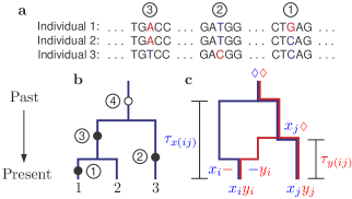
Figure 1: Gene history and polymorphic sites. a In DNA, genetic information is encoded by base-pairs of the four nucleic acids adenine (A), thymine (T), guanine (G), and cytosine (C). In a sample of three individuals, we show three polymorphic sites, with two nucleotides around each polymorphism. b The most common variation is a difference at a single position (SNP), caused by a mutation at the position in an individual in the history of the population, where e.g. a fraction of the population has the nucleotide T at the site, and the rest has the nucleotide A. The three mutations in panel a are shown as filled circles. Mutation 4 does not cause a polymorphism in the sample, since all individuals in the sample inherits the mutation from the common ancestor. Given $\tau$ (the number of generations since the most recent common ancestor) of a stretch of $L$ nucleotides, the number of differences between two individuals is assumed to be Poisson distributed with expected value $2\mu L\tau$, where $\mu$ is the mutation rate per site per generation [1]. c In recombination, part of a gamete (one of the two copies of a chromosome) is inherited from one parent and the rest from the other parent. We show a sample gene history with one recombination event, for two loci ($x$ and $y$) in two gametes $i$ and $j$. The time axis is the same as in panel b. The ancestral history for loci $x$ and $y$ are shown in blue and red, respectively. The times until the most recent common ancestor are $\tau_{x(ij)}$ and $\tau_{y(ij)}$ for loci $x$ and $y$, respectively. In the absence of recombination, two loci on the same gamete share the same genetic history, and have the same time to the most recent common ancestor, $\tau_{x(ij)}=\tau_{y(ij)}$, causing linkage disequilibrium. If a recombination event occurs in the genetic history of a sample, it may lead to a decorrelation of $\tau_{x(ij)}$ and $\tau_{y(ij)}$. $x_{i}$ represents the genetic material at locus $x$ of chromosome $i$. Dashes correspond to genetic material not in the history of the sample, and the diamonds to common ancestral material.

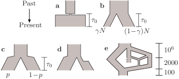
Figure 2: Models illustrating demographic history, i.e. changes in population size and structure. a Population bottleneck. b,c Models of population structure and expansion. d A more general model of demographic structure. e Demographic structure determining genetic variation in the laboratory-mouse genome [30] (time here is measured in years).

2 Gene-history correlations, linkage disequilibrium, and patterns of genetic variation

Genetic variation is caused by multiple factors. Together, mutations and recombination (figure 1) are the most important determinants of the large-scale haplotype structure in the human genome [3, 12, 4]. The genetic history of nearby sites is closely related, while distant sites may become unrelated only a few generations in the past.

Correlation of gene histories determines the degree of association between patterns of genetic variation at different loci. An example is the correlation of the counts of single-nucleotide polymorphisms (SNPs) at different loci: let $S_{x(ij)}$ be the number of SNPs at locus $x$ between a pair of chromosomes $i$ and $j$. Further, let $\tau_{x(ij)}$ denote the time to the most recent common ancestor of a locus at position $x$ on chromosomes $i$ and $j$, and define $\tau_{y(ij)}$ correspondingly for the locus at position $y$. Then the sample covariance of the number of SNPs in non-overlapping loci $x$ and $y$ is related to the covariance of times $\tau_{x(ij)}$ and $\tau_{y(ij)}$ as follows

$$\mathrm{cov}[S_{x(ij)},S_{y(ij)}]\approx(2\mu L)^{2}\,\mathrm{cov}[\tau_{x(ij)},\tau_{y(ij)}]\,.$$ (1)

Here $L$ is the size of the loci, assuming variations in the mutation rate $\mu$ along the chromosome are negligible. For (1) to hold, $L$ must be small enough that the sites within each locus have a high degree of linkage (in humans, $L$ must be of the order of or smaller than a few hundred base-pairs).

Associations between SNPs in the genetic mosaic allows for efficient mapping of genes. Suitably chosen, a relatively small set of SNPs can capture most of the common patterns of variation in the genome [4].

The decay of the covariance $\mbox{cov}[\tau_{x(ij)},\tau_{y(ij)}]$ as a function of $|x-y|$ measures linkage disequilibrium. In the remainder of this section we briefly comment on other common measures of linkage disequilibrium. Global association between patterns of diversity, quantified by the extent of linkage disequilibrium is often measured by Tajima’s $D^{\prime}$ [5] or alternatively by

$$r^{2}=\frac{D^{2}}{f_{A(x)}(1-f_{A(x)})f_{B(y)}(1-f_{B(y)})},$$ (2)

where $D=f_{A(x)B(y)}-f_{A(x)}f_{B(y)}$, $A(x)$ and $B(y)$ are the allelic types at the loci $x$ and $y$, respectively, and $f_{A(x)B(y)}$ is frequency of alleles $A(x)$ and $B(y)$ on the same chromosome in the sample [5]. McVean [23] introduced an approximation to the expected value of $r^{2}$, called $\sigma^{2}_{d}$, which makes the connection to the correlation of gene history explicit. With the notation $E_{ij,kl}=\langle\tau_{x(ij)}\tau_{y(kl)}\rangle$,

$$\sigma^{2}_{d}=\frac{(n^{2}-2n+2)E_{ij,ij}-2(n-2)^{2}E_{ij,ik}+(n-2)(n-3)E_{ij,kl}}{2E_{ij,ij}+4(n-2)E_{ij,ik}+(n-2)(n-3)E_{ij,kl}}\,.$$ (3)

The factors $E_{ij,ij}$ and $E_{ij,ik}$ are defined analogously. For unstructured populations, $\sigma^{2}_{d}$ and the expected value of $r^{2}$ are approximately equal under the neutral dynamics, if the expectation is conditioned on intermediate allelic frequencies [23].

3 Methods

In the following we analyse how correlation of gene histories depends on demographical factors. In a large, unstructured population with constant population size, and when selection is negligible, the ancestral history of a locus may be modeled as a Markov process [26, 27, 2], where the states of the process correspond to different configurations of ancestral DNA through the history of the sample.

We trace the ancestral history of two loci (at positions $x$ and $y$) in $n$ individuals, from the present back in time until the most recent common ancestor has been found for all loci. When the population size $N$ is large, the genealogical process may be approximated by the so-called coalescent process [1]: recombination is modeled as a Poisson process with rate $r$ per generation per chromosome: for any given chromosome, with probability $r$ (also known as the recombination fraction) the loci stem from different parents. The probability that one pair of individuals has a common ancestor in the preceding generation, and the probability that an individual inherits genetic material from both parents, are expanded in $N^{-1}$ to the first order. Time is measured in units of $2N$ generations. In the limit of large $N$, the time to the next event is approximately exponentially distributed [1].

By explicitly taking into account the symmetries of the state space of the coalescent for two individuals, we obtain a compact representation of the Markov process (figure 3) which allows us to derive and understand gene-history correlations in the models mentioned in the introduction.

We illustrate our approach by re-deriving Hudson’s result for the correlation of gene histories in the unstructured, constant population-size coalescent model [15]. Consider a sample of two individuals. Figure 3 shows a representation of the coalescent for this case. Each node in the graph corresponds to a configuration of ancestral DNA (listed in the table in figure 3). Due to the symmetries of the coalescent, many different configurations may be mapped onto the same node.

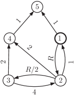
State $i\$ Population $1$ $x_{i}y_{i}$, $x_{j}y_{j}$ $x_{i}y_{j}$, $x_{j}y_{i}$ $2$ $x_{i}-$, $-y_{i}$, $x_{j}y_{j}$ $x_{i}y_{i}$, $x_{j}-$, $-y_{j}$ $x_{i}-$, $-y_{j}$, $x_{j}y_{i}$ $x_{i}y_{j}$, $x_{j}-$, $-y_{i}$ $3$ $x_{i}-$, $-y_{i}$, $x_{j}-$, $-y_{j}$ $4$ $x_{i}\scriptstyle\lozenge$, $x_{j}\scriptstyle\lozenge$ ${\scriptstyle\lozenge}y_{i}$, ${\scriptstyle\lozenge}y_{j}$ $5$ $\scriptstyle\lozenge\lozenge$

Figure 3: A graph representation of the coalescent process for two loci ($x$ and $y$) and two chromosomes ($i$ and $j$). The transition rates (measured in units of $2N$ generations) between the different groups of states, corresponding to the table, are printed along the arrows ($R=4Nr$). The process starts in state $1$ and ends in state $5$, the only absorbing state. If the path goes from state $1$ to state $5$ we have linkage, but if the system enters state $4$ linkage is broken. Same notation as in figure 1.

The time evolution of the probability distribution $P_{i}(t)$ over the states $i$ is given by the master equation

$$\partial_{t}P_{i}(t)=\sum_{j}w_{j\rightarrow i}P_{j}(t)-\sum_{j}w_{i\rightarrow j}P_{i}(t)\,,$$ (4)

where $w_{i\rightarrow j}$ is the transition rate from state $i$ to state $j$, given in figure 3. As above, time is measured in units of $2N$ generations. The process is started in state $1$, and proceeds until it comes to state $5$. We find that $\langle\tau_{x(ij)}\tau_{y(ij)}\rangle$ is given by the exit rates to state $5$, via states $1$ and $4$. Let $\tau_{1}$ be the first time at which a locus coalesces, and $\tau_{2}$ be the time when both loci have coalesced. Since $\tau_{x(ij)}\tau_{y(ij)}=\tau_{1}\tau_{2}$ we obtain

$$\left<\tau_{x(ij)}\tau_{y(ij)}\right>=\int_{0}^{\infty}\Big{[}{\bm{u}}_{1}^{\mathrm{T}}\tau_{1}^{2}+{\bm{u}}_{2}^{\mathrm{T}}\!\int_{\tau_{1}}^{\infty}\tau_{1}\tau_{2}\,{\rm e}^{\tau_{1}\!-\!\tau_{2}}\,\rmd\tau_{2}\Big{]}{\rm e}^{{\bf M}\tau_{1}}\,{\bm{v}}\,\rmd\tau_{1}\,,$$ (5)

where ${\bm{v}}={\bm{u}}_{1}=(1,0,0)^{\mathrm{T}}$, ${\bm{u}}_{2}=(0,2,2)^{\mathrm{T}}$ and $\mathbf{M}$ is a three-by-three matrix defined by $\mathbf{M}_{ij}=w_{j\rightarrow i}$ for $i,j=1,\dots,3$ and $i\neq j$, and $M_{ii}=-\sum_{j=1}^{3}w_{i\rightarrow j}$. Evaluating (5) we obtain the well-known result [27, 15]

$$\rho(\tau_{x(ij)},\tau_{y(ij)})\equiv\frac{\left<\tau_{x(ij)}\tau_{y(ij)}\right>-\left<\tau\right>^{2}}{\left<\tau^{2}\right>-\left<\tau\right>^{2}}=\frac{R+18}{R^{2}+13R+18}\,,$$ (6)

where $R=4Nr$. In order to calculate $\sigma^{2}_{d}$ for the unstructured model, we obtain $\langle\tau_{x(ij)}\tau_{y(ik)}\rangle$ and $\langle\tau_{x(ij)}\tau_{y(kl)}\rangle$ from (5) with ${\bm{v}}=(0,1,0)^{\mathrm{T}}$ and ${\bm{v}}=(0,0,1)^{\mathrm{T}}$, respectively. Inserting these into eq. (3), we recover the result of McVean [23]:

$$\sigma^{2}_{d}=\frac{2\,(6+R)+n\,(10+11R+R^{2})+n^{2}(10+R)}{2\,(6+R)-n\,(14+13R+R^{2})+n^{2}(22+13R+R^{2})}.$$ (7)

In the following, we consider models corresponding to Markov processes with rates which are piece-wise constant functions of time $t$. This allows us to calculate $\langle\tau_{x(ij)}\tau_{y(ij)}\rangle$ from (5) by taking $\mathbf{M}$ and ${\bm{u}}$ to be functions of time.

4 Results

After having illustrated our approach, we now briefly describe the demographic models we have considered and summarise our results for gene-history correlations in these models. Mathematical details are given in appendices A and B. Implications are discussed in section 5.

4.1 Bottleneck model

Consider (c.f. [28]) an unstructured population of constant size $N$ until $\tau_{0}=2NG$ generations ago. The population was then subject to a severe bottleneck of short duration, followed by a rapid expansion to a very large (infinite) population size (figure 2a). Between the bottleneck and now, the population size is taken to be effectively infinite: and thus the probability that two randomly sampled individuals have a common ancestor before the bottleneck is negligible. Since the bottleneck is very narrow and has a short duration, we may ignore the effect of recombination during the bottleneck. It is convenient to parameterise the duration of the bottleneck in terms of the probability $F$ that a single locus coalesces during the bottleneck. In the limit when both the population size and duration of the bottleneck are small (compared to $2N$ individuals and generations, respectively), we obtain (appendix A):

$$\rho(\tau_{x(ij)},\tau_{y(ij)})=\frac{A+B\,e^{-RG/2}+C\,e^{-RG}}{15\,(2-h)\,(18+13\,R+R^{2})}\,,$$ (8)

where $h=1-F$ and

$$A = 6(36-45h+20h^{2}-h^{5})+3(28-65h+$$ (9)

$$+\ 40h^{2}-3h^{5})R+{(1-h)}^{3}(6+3h+h^{2})R^{2}\,,$$

$$B = 12(9-5h^{2}+h^{5})+(3-5h^{2}+2h^{5})R^{2}$$ (10)

$$+\ 6(7-10h^{2}+3h^{5})R\,,$$

$$C = 6(36-10h^{2}-h^{5})+(6-5h^{2}-h^{5})R^{2}$$ (11)

$$+\ 3(28-20h^{2}-3h^{5})R\,.$$

We thus find that this model exhibits correlations at arbitrarily large values of $R$, a consequence of an infinite expansion rate after the bottleneck, and negligible recombination within it. If, instead, the expansion were to a finite population size, (smaller than $GN$, say), the correlations would still converge to a constant at large $R$. The constant, however, is expected to be lower than the asymptotic value obtained from (4) as $R\rightarrow\infty$. Finally, if the bottleneck lasts long enough for significant recombination to occur within it, we still find long-range correlations, up to scales of the order of $(2\tau_{\rm D}r)^{-1}$ where $\tau_{\rm D}$ is the duration of the bottleneck (in generations). Beyond this, the correlations decay, and in the limit $R\rightarrow\infty$ we have $\rho(\tau_{x(ij)},\tau_{y(ij)})\rightarrow 0$ as in the unstructured population model.

By the same approach, we calculate $\langle\tau_{x(ij)}\tau_{y(ik)}\rangle$ and $\langle\tau_{x(ij)}\tau_{y(kl)}\rangle$. Inserting this into (3) yields, for large $n$:

$$\sigma^{2}_{d} = \frac{e^{-G\,R}}{\langle\tau_{x(ij)}\tau_{y(kl)}\rangle}\Big{[}18\,h\,(36-10\,h^{2}-h^{5})+9\,h\,(28-20\,h^{2}-3\,h^{5})\,R+$$ (12)

$$3\,h\,(6-5\,h^{2}-h^{5})\,R^{2}\Big{]}\,,$$

where

$$\langle\tau_{x(ij)}\tau_{y(kl)}\rangle = 18\,(45\,G^{2}+36\,h+90\,G\,h+20\,h^{3}-h^{6})+$$ (13)

$$9\,(65\,G^{2}+28\,h+130\,G\,h+40\,h^{3}-3\,h^{6})\,R+$$

$$(45\,G^{2}+18\,h+90\,G\,h+30\,h^{3}-3\,h^{6})\,R^{2}\,.$$

Note that $\sigma^{2}_{d}\rightarrow 0$ as $R\rightarrow\infty$. The difference, in particular, to expression (7) is not large. Hence, when the aim is to detect the population-size variations it is better to focus on single-locus statistics.

4.2 Model of divergent populations, I

Reich et al. consider a model of a diverging population [3]: the population was unstructured with constant population size $N$ until $\tau_{0}=2NG$ generations ago, when the the population split into two parts of equal size $N$ (note that this implies a rapid population expansion from $N/2$ to $N$ after the split). The model is illustrated in figure 2c. A portion $p$ of the sample is chosen from the first population, and the rest from the second population. For any two individuals in the sample, the expectation $\rho(\tau_{x(ij)},\tau_{y(ij)})$ depends on whether the individuals come from the same sub-population or not. Using the technique illustrated above, it is straightforward to calculate the expectation for both cases. Again, we find long-range correlations, namely

$$\rho(\tau_{x(ij)},\tau_{y(ij)})=1-\frac{1}{1+2\,p\,(1-p)\,(1-2\,p+2\,p^{2})\,G^{2}}\,,$$ (14)

in the limit of large $R$ (in appendix B we describe how to obtain the full result, valid for arbitrary values of $R$).

Further, in the limit of large $R$ and large sample size $n$, we have

$$\sigma^{2}_{d}=\frac{2\,p^{2}\,(1-p)^{2}\,G}{1+2\,p\,(1-p)\,G}.$$ (15)

Thus, for this model $\sigma^{2}_{d}$ is finite in the limit of large $R$, as opposed to $\sigma^{2}_{d}$ in the unstructured model (section 2) and the bottleneck model (section 4.1).

4.3 Model of divergent populations, II

Now consider the model of two diverging sub-populations [28] in figure 2b. The population was unstructured with constant size of $N$ individuals until $\tau_{0}=2NG$ generations ago, when a fraction $\gamma$ of the population diverged. In subsequent generations, the two sub-populations where unstructured but with no contact between sub-populations. Individuals are randomly chosen from the joint population. For two individuals in the sample, there are three cases: both individuals may come from the smaller sub-population, they may come from the larger sub-population, or from different sub-populations. Using equation (5) we find long-range correlations: in the limit of large $R$, $\rho$ remains finite,

$$\rho(\tau_{x(ij)},\tau_{y(ij)}) = \frac{1}{\mbox{var}[\tau]}\big{[}1-2s+2s^{2}+2G\left(2+G\right)s+s^{2}{\rm e}^{-\frac{2G}{\gamma}}+$$

$$s^{2}{\rm e}^{-\frac{2G}{1-\gamma}}+2s{\left(1-\gamma\right)}^{2}{\rm e}^{-\frac{G}{1-\gamma}}+2s{\gamma}^{2}e^{-\frac{G}{\gamma}}-\left<\tau\right>^{2}\big{]}\,$$

where $s=\gamma\,(1-\gamma)$ and

$$\left<\tau\right> = 1+s(2G-1)+s\gamma{\rm e}^{-\frac{G}{\gamma}}+s(1-\gamma){\rm e}^{-\frac{G}{1-\gamma}}\,$$ (17)

$$\mbox{var}[\tau] = 2+2s\big{[}2s+(G+1)^{2}+\gamma(1+G+\gamma){\rm e}^{-\frac{G}{\gamma}}+$$ (18)

$$+\ (1-\gamma)(2+G-\gamma){\rm e}^{-\frac{G}{1-\gamma}}-3\big{]}-\left<\tau\right>^{2}\,.$$

See the appendix for the full result. The long-range correlations are found to be due to sampling of different sub-populations.

In the limit of large $R$ and large sample size, we have

$$\sigma^{2}_{d}=\frac{\gamma^{2}(1-\gamma)^{2}}{\langle\tau\rangle^{2}}\left[2\,G+\gamma\,(1-\rme^{-\frac{G}{1-\gamma}})+(1-\gamma)(1-\rme^{-\frac{G}{\gamma}})\right]^{2}.$$ (19)

Again, we find that $\sigma^{2}_{d}$ is finite in the limit of large $R$.

5 Discussion

Figure 4 shows the correlations $\rho(\tau_{x(ij)},\tau_{y(ij)})$ in the demographic models considered, with parameters chosen to be consistent with the empirically estimated time to the most recent common ancestor and its coefficient of variation [3]. When plotting the correlation of gene histories against physical positions, we need to translate the recombination fraction $r$ into the corresponding expected number $\sigma x$ of crossover events between the two loci. There are many such maps proposed in the literature (see e.g. [29] for a review of these). They differ in how they model the chiasma process, but all models have in common that for small enough $r$, $r\approx\sigma x$. In humans, $r\approx\sigma x$ for $x\lesssim 10^{6}$bp. At larger distances, deviations from linearity are not noticeable since the expressions for $\rho(\tau_{x(ij)},\tau_{y(ij)})$ and $\sigma^{2}_{d}$ converge for large $R$ (to different values, in general). Also shown are empirical estimates of lower and upper bounds on the correlation of gene histories in the human genome [3]. The correlations for the models described in section 4 are substantially larger at large distances than those for the unstructured model, but they lie significantly below the lower bound of the empirical data, at intermediate distances. We comment on possible causes for this discrepancy in our conclusions.

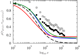
Figure 4: Correlation $\rho(\tau_{y(ij)},\tau_{(y+x)(ij)})$ of gene histories as a function of the distance $x$ between them. Equations (6), (8), and exact expressions corresponding to (14) and (4.3), from the appendix, were used. In all cases, $r=1.2$ cM/Mb, $N$ and $\mu$ were chosen to be consistent with $2N\left<\tau\right>=1.55\times 10^{4}$, and a coefficient of variation of $0.94$ [3] (except in the unstructured model). The lines are: the unstructured coalescent (dashed), bottleneck model with $H=0.1$ (red), divergent model in figure 2b with $\gamma=0.2$ (blue), and divergent model in figure 2c with $p=0.3$ (green). Also shown are empirical estimates of lower and upper bounds for the correlation of gene histories in the human genome (squares) [3].

Our results allow us to gain a qualitative understanding of the influence of demographic factors on the decorrelation of gene histories. First, we find that models of bottlenecks and divergent populations (figure 2) both exhibit long-range correlations in gene histories, as numerically demonstrated in [3], but for very different reasons. In bottlenecks, the length scale at which we find significant correlations is governed by the degree of recombination within the bottleneck: low recombination in the bottleneck gives rise to long-range correlations. Further, the amount of correlation is affected by the rate of expansion of the population after the bottleneck: rapid expansion gives high correlations. Long-range correlation in divergent models, on other hand, we ascribe to the fact that the covariance of $\tau_{x(ij)}$ and $\tau_{y(ij)}$ (that is, the number of generations since the common ancestor of two copies of loci $x$ and $y$) is different when individuals are selected from the same or different sub-populations: typically, the covariance is lower for individuals from the same sub-population than from different ones. We find that this effect persists even for loci far apart, but is decreased by population expansions during the divergence.

Second, we identify two contributions to the correlation of gene histories in divergent populations: linkage disequilibrium and the sampling of sub-populations with different demographic histories. At short ranges, linkage disequilibrium correlates nearby patterns by co-inheritance. Thus, for small distances, we conclude that the demographic structure is unimportant: all reasonable models must give high correlation for small distances. For long ranges, by contrast, correlations due to linkage disequilibrium are expected to vanish, but the contribution from differences in gene history across sub-populations remains.

Third, the domestication of crops and animals has shaped the genetic makeup of the species, through selection for desirable traits but also through the demographic history of each species [28]. The pattern of genetic differences in the laboratory mouse population depends strongly on its demographic history [30]. In divergent populations, we find that long-range correlations are insensitive to the demographic history of the sub-populations. As a consequence, we predict that the most important contribution to the correlation of gene history in the laboratory mouse is from the original divergence from the wild-type mouse.

Fourth, we found that within the models described in section 4, gene-history correlations are substantially increased as compared with the unstructured, standard model. However, the correlations still lie significantly below the empirically determined data at intermediate distances. In [25] it was shown that incorporating empirically observed variations in the recombination-rate along the chromosomes [24] significantly increases the correlations in this regime. Our analytical expressions for the correlation of gene histories allow for studying the effect of such variations in the recombination rate in models with demographic population structure.

Fifth, we briefly mention possible extensions of the scheme introduced in this paper. In more general sampling schemes (different from those depicted in figure 2), we may use the expressions for $\left<\tau_{x(ij)}\,\tau_{y(ij)}\right>$ conditional on whether the individuals in the sample came from the same sub-population or not, and conditional on the population size during the divergence, to calculate the correlation of gene histories by weighting the different contributions by the probability that they occur under the sampling scheme. Also, it is straight-forward to extend the calculations to combinations of bottlenecks and divergent populations (figure 2d), and to more complicated models involving more than two diverging branches (figure 2e). It is expected that the most distant (symmetric) divergence determines the long-range correlations.

How would a recent mixing event (figure 2e) affect the correlation of gene histories? A merging of the divergent populations $g$ generations ago leads to a decorrelation of gene histories at distances of the order of $(4gr)^{-1}$, since then ancestral lines of both loci may come from different sub-populations with approximately equal probability.

Finally, we have argued that the correlation $\rho(\tau_{x(ij)},\tau_{y(ij)})$ of gene histories determines the association of SNP counts, $\mbox{cov}[S_{x(ij)},S_{y(ij)}]$. Conversely one may be interested in estimating model parameters from population data, deducing $\rho(\tau_{x(ij)},\tau_{y(ij)})$ from the pairwise statistic $\mbox{cov}[S_{x(ij)},S_{y(ij)}]$. Three questions arise. First, how can one in practice estimate $\mbox{cov}[\tau_{x(ij)},\tau_{y(ij)}]$ from the variance of SNP counts? Second, how good is this estimate? Third, how much of the information the full data set (possibly pertaining to a large number of individuals) is retained in the pair-wise statistic $\mbox{cov}[S_{x(ij)},S_{y(ij)}]$? We begin by answering the last question. Due to the high amount of association between the chromosomes in a sample, the information on genealogical history accumulates slowly as the sample size is increased [17]. It follows that most information can be found in pair-wise comparisons between the chromosomes in the sample as used in eq. (1). Going back to the first two questions, an estimator for $\rho(\tau_{y(ij)},\tau_{(y+x)(ij)})$ can be constructed as follows. Assuming that the length $L_{\mathrm{c}}$ of the sequences is long, we can estimate the correlation of polymorphism rates by averaging over all pairs and positions:

$$\rho(\tau_{y(ij)},\tau_{(y+x)(ij)})\approx\hat{\rho}(x)=\frac{\overline{S_{y}S_{y+x}}-\overline{S_{y}}^{2}}{\overline{S_{y}^{2}}-\overline{S_{y}}^{2}-\overline{S_{y}}},$$ (20)

where

$$\overline{S_{y}S_{y+x}}=\frac{2}{n(n-1)(L_{\mathrm{c}}-x-L)}\sum_{i=2}^{n}\sum_{j=1}^{i-1}\sum_{y=1}^{L_{\mathrm{c}}-x-L}S_{y(ij)}S_{(y+x)(ij)}\,.$$ (21)

and the single-locus quantities $\overline{S_{y}}$ and $\overline{S_{y}^{2}}$ are defined similarly. Instead of regularly spaced bins, as in (21), one may use randomly positioned bins. For unstructured populations, and for populations with bottlenecks and expansions, the accuracy of the estimator $\hat{\rho}(x)$ depends mostly on the number of bins (and hence on $L_{\mathrm{c}}$), and improves only slowly with increasing $n$. For divergent models, however, increasing $n$ improves the sampling from the different sub-populations. In figure 5 we show how $\hat{\rho}(x)$ compares to $\rho(\tau_{y(ij)},\tau_{(y+x)(ij)})$ when applied to a sample. As can be seen in the figure, when $x<L$ the bins overlap and $\hat{\rho}(x)$ overestimates the correlations, but otherwise it works well.

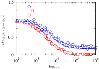
Figure 5: Comparison of $\hat{\rho}(x)$ (markers) to $\rho(\tau_{y(ij)},\tau_{(y+x)(ij)})$ (solid lines, calculated from theory), for an unstructured population (red) and a divergent population (blue). The estimator $\hat{\rho}(x)$ were obtained from a single sample of 50 individuals, with $L_{\mathrm{c}}=10$Mb, for different bin sizes $L=100$bp (diamonds), $L=500$bp (circles) and $L=1$kb (squares). The parameters for the divergent model are: $G=0.6$, $p=0.3$, $N=6963.7$, $r=0.95633$cM/Mb, $\theta=7.6\,10^{-4}$. In the unstructured population model, the population size is $N=10^{4}$.

6 Conclusions and outlook

We have derived closed analytical expressions for the correlation of gene histories in established demographic models for genetic evolution. These expressions allow us to understand and quantitatively determine how demographical factors give rise to long-range correlations in gene histories.

The correlations analysed here determine the two-person summary statistic (1). More information is contained in the mosaics of SNP haplotype patterns for more than two individuals, and their associations [17]. It is of great interest to derive corresponding expressions for correlations between such patterns in the models considered in this paper, especially in the case of more than two loci. Finally we note that the quantity $\sigma_{d}^{2}$, a measure of linkage disequilibrium, was shown to be a good approximation to $r^{2}$ in the case of unstructured populations [18]. It is necessary to investigate the relation between $r^{2}$ and $\sigma^{2}_{d}$ in models with demographic structure.

Appendix A: Derivation of bottleneck formula

During the bottleneck, the time between coalescent events is exponentially distributed with rate ${n\choose 2}/(2\,\gamma N)$, where $n$ is the number of lines carrying ancestral material. Recombination events occurs with rate $n\,R/(4N)$, independent of $\gamma$. Thus when $\gamma$ is very small, coalescent events dominate the process.

We assume that during the bottleneck, the reduction in effective population size is so drastic that $\gamma$ is effectively zero. By rescaling the time by a factor of $\gamma$ and taking the limit of $\gamma\rightarrow 0$ we find

$$\mathbf{M}^{\prime}=\lim_{\gamma\rightarrow 0}\mathbf{M}(\gamma)\,\gamma=\left[\begin{array}[]{rrr}-1&1&0\\ 0&-3&4\\ 0&0&-6\end{array}\right],$$ (25)

so the time evolution operator becomes

$$\exp(\mathbf{M}^{\prime}\,t)=\left[\begin{array}[]{rrr}e^{-t}&\frac{1}{2}\,e^{-t}-\frac{1}{2}\,e^{-3t}&\frac{2}{5}\,e^{-t}-\frac{2}{3}\,e^{-3t}+\frac{4}{15}\,e^{-6t}\\ 0&e^{-3t}&\frac{4}{3}\,e^{-3t}-\frac{4}{3}\,e^{-6t}\\ 0&0&e^{-6t}\\ \end{array}\right].$$ (29)

In the original model, the inbreeding coefficient $F$ was specified. We choose to parameterise the severity of the bottleneck by its duration $D$. If the process is in state $1$ (figure 3) when entering the bottleneck, the probability of coalescence during the bottleneck is

$$\int_{0}^{D}{\bm{u}}_{1}^{\mathrm{T}}\,\rme^{\mathbf{M}^{\prime}\,t}\,{\bm{u}}_{1}\,\rmd t=1-\rme^{-D},$$ (30)

so we see that by taking $D=-\ln(1-F)$, we get the correct inbreeding coefficient. We can now express the time evolution operator from the beginning to the end of the bottleneck as

$$\exp(\mathbf{M}^{\prime}\,D)=\left[\begin{array}[]{rrr}H&\frac{1}{2}\,H\,(1-H^{2})&\frac{2}{15}\,H\,(3-5\,H^{2}+2\,H^{5})\\ 0&H^{3}&\frac{4}{3}\,H^{3}\,(1-H^{3})\\ 0&0&H^{6}\end{array}\right],$$ (34)

where $H=1-F$. The probability that the loci become linked during the bottleneck depends on the state of the process when the bottleneck is entered:

$$\int_{0}^{D}{\bm{u}}_{1}^{\mathrm{T}}\,\rme^{\mathbf{M}^{\prime}\,t}\,\rmd t=\left\{\begin{array}[]{ll}F&\mbox{in state $1$}\\ \frac{1}{6}\,(2+H)\,F^{2}&\mbox{in state $2$}\\ \frac{2}{45}\,(5+6\,H+3\,H^{2}+H^{3})\,F^{3}&\mbox{in state $3$}\end{array}\right.$$ (38)

Similarly, we have the probability that one locus, but not the other, reaches its most recent common ancestor during the bottleneck, depending on the state of the process when entering the bottleneck:

$$\int_{0}^{D}{\bm{u}}_{2}^{\mathrm{T}}\,\rme^{\mathbf{M}^{\prime}\,t}\,\rmd t=\left\{\begin{array}[]{ll}0&\mbox{in state $1$}\\ \frac{2}{3}\,(1-H^{3})&\mbox{in state $2$}\\ \frac{1}{9}\,(7-8\,H^{3}+H^{6})&\mbox{in state $3$}\end{array}\right.$$ (42)

Together, (34), (38) and (42) determines the state of the process after the bottleneck. Using this information and the method for the unstructured population as outlined in section 2 allows us to derive the gene-history correlation for the bottleneck model.

Appendix B: Correlation of gene histories in divergent populations

Assume that individuals come from left sub-population with probability $p$ and from the right one with probability $1-p$. The population size in the left and right sub-populations are $\gamma N$ and $\Gamma N$, respectively, and the population size before the divergence is $N$. The two-person coalescent process is described by a Markov process over the states in table 1, where state $1$ is the absorbing state of the process, and the process starts in one of states $3-11$.

Table 1: The states of the Markov process of loci $x$ and $y$ in chromosomes $i$ and $j$, for the divergent population. For each state we show the corresponding configurations of the sub-populations, separated by a vertical bar. A dash denotes genetic material that is not ancestral to any locus in the sample. The symbol $\phi$ denotes a sub-population unrelated to sample, and the diamonds denotes a common ancestor to chromosomes $i$ and $j$ (for that locus).

• State	Population configuration
  0	$\phi$ $|$	$\phi$
  1	$x_{i}\diamond$, $x_{j}\diamond$ $|$	$\phi$
  2	$x_{i}\diamond$ $|$	$x_{j}\diamond$
  3	$x_{i}y_{i}$, $x_{j}y_{j}$ $|$	$\phi$
  4	$x_{i}y_{i}$ $|$	$x_{j}y_{j}$
  5	$x_{i}y_{i}$, $x_{j}-$, $-y_{j}$ $|$	$\phi$
  6	$x_{i}y_{i}$, $x_{j}-$ $|$	$-y_{j}$
  7	$x_{i}y_{i}$ $|$	$x_{j}-$, $-y_{j}$
  8	$x_{i}-$, $-y_{i}$, $x_{j}-$, $-y_{j}$ $|$	$\phi$
  9	$x_{i}-$, $-y_{i}$, $x_{j}-$ $|$	$-y_{j}$
  10	$x_{i}-$, $-y_{i}$ $|$	$x_{j}-$, $-y_{j}$
  11	$x_{i}-$, $x_{j}-$ $|$	$-y_{i}$, $-y_{j}$

We now define $e_{i}=\langle\,\tau_{1}\tau_{2}\,|\,\mbox{Process starting in state $i$}\,\rangle$. With these, we may write

$$\langle\tau_{x(ij)}\tau_{y(ij)}\rangle = p^{2}\,e_{3}(\gamma)+(1-p)^{2}\,e_{3}(\Gamma)+2p(1-p)\,e_{4}(\gamma,\Gamma),$$ (43)

$$\langle\tau_{x(ij)}\tau_{y(ik)}\rangle = p^{3}\,e_{5}(\gamma)+(1-p)^{3}\,e_{5}(\Gamma)$$ (44)

$$+ 2p(1-p)^{2}\,e_{6}(\gamma)+2p^{2}(1-p)\,e_{6}(\Gamma)$$

$$+ p(1-p)^{2}\,e_{7}(\gamma,\Gamma)+p^{2}(1-p)\,e_{7}(\Gamma,\gamma),$$

$$\langle\tau_{x(ij)}\tau_{y(kl)}\rangle = p^{4}\,e_{8}(\gamma)+(1-p)^{4}\,e_{8}(\Gamma)$$ (45)

$$+ 4p^{3}(1-p)\,e_{9}(\gamma)+4p(1-p)^{3}\,e_{9}(\Gamma)$$

$$+ 4p^{2}(1-p)^{2}\,e_{10}(\gamma,\Gamma)+2p^{2}(1-p)^{2}\,e_{11}(\gamma,\Gamma).$$

From this, the correlation $\rho(\tau_{x(ij)},\tau_{y(ij)})$ and $\sigma^{2}_{d}$ may be calculated for both models of divergent populations: setting $\gamma=\Gamma=1$ gives the model described in section 4.2; setting $\Gamma=1-\gamma$ and $p=\gamma$ gives the model described in section 4.3.

Calculation of $e_{3},\ldots,e_{11}$ for the model introduced in section 4.2

The two-locus coalescent in a population of size $\gamma N$ is described by a Markov process with the evolution matrix

$$\mathbf{M}_{1}=\left[\begin{array}[]{ccc}-1/\gamma-R&1/\gamma&0\\ R&-3/\gamma-R/2&4/\gamma\\ 0&R/2&-6/\gamma\end{array}\right]\!\!.$$ (46)

where $R=4Nr$. Before the divergence, $\gamma=1$ and we denote the corresponding evolution matrix $\mathbf{M}$. the coalescent is described by a Markov process with the evolution matrix $\mathbf{M}$. Assuming that population is in state $3$, $5$, or $8$ with probabilities $v_{1}$, $v_{2}$, and $v_{3}$, respectively, we proceed as for the unstructured population in section 3, calculating $\langle\tau_{1}\tau_{2}\rangle$ conditional on starting from distribution ${\bm{v}}$. We obtain $e_{3}(\gamma)=c_{\mathrm{s}}(\gamma,(1,\,0,\,0)^{\mathrm{T}})$, $e_{5}(\gamma)=c_{\mathrm{s}}(\gamma,(0,\,1,\,0)^{\mathrm{T}})$, and $e_{8}(\gamma)=c_{\mathrm{s}}(\gamma,(0,\,0,\,1)^{\mathrm{T}})$, where

$$c_{\mathrm{s}}(\gamma,{\bm{v}}) = \frac{{\bm{u}}_{1}^{\mathrm{T}}}{\gamma}\,(-\mathbf{M}_{1})^{-3}\,\big{[}2\,\mathbf{I}-(2\,\mathbf{I}-2\,\frac{G}{\gamma}\,\mathbf{M}_{1}+\frac{G^{2}}{\gamma^{2}}\,\mathbf{M}_{1}^{2})\,\exp\!\big{(}\mathbf{M}_{1}G\big{)}\big{]}{\bm{v}}$$ (47)

$$+ {\bm{u}}_{1}^{\mathrm{T}}\,(-\mathbf{M})^{-3}\,\big{(}2\,\mathbf{I}-2\,G\,\mathbf{M}+G^{2}\,\mathbf{M}^{2}\big{)}\,\exp\!\big{(}\mathbf{M}_{1}G\big{)}{\bm{v}}$$

$$+ \frac{{\bm{u}}_{2}^{\mathrm{T}}}{\gamma}\,(-\mathbf{M}_{1})^{-3}\Big{\{}2\,\mathbf{I}-\gamma\,\mathbf{M}_{1}-\left[2\,\mathbf{I}-(2\,G+\gamma)\,\mathbf{M}_{1}+G\,(G+\gamma)\,\mathbf{M}_{1}^{2}\right]\exp\!\big{(}\mathbf{M}_{1}G\big{)}\Big{\}}{\bm{v}}$$

$$+ (1-\gamma)\,{\bm{u}}_{2}^{\mathrm{T}}\,(\mathbf{I}+\gamma\,\mathbf{M}_{1})^{-2}\,\Big{\{}\gamma\,e^{-G/\gamma}\,\mathbf{I}+\left[\,(G-\gamma)\,\mathbf{I}+\gamma\,G\,\mathbf{M}_{1}\,\right]\,\exp\!\big{(}\mathbf{M}_{1}G\big{)}\Big{\}}{\bm{v}}$$

$$+ {\bm{u}}_{2}^{\mathrm{T}}(-\mathbf{M})^{-3}\left[2\,\mathbf{I}-(1+2\,G)\,\mathbf{M}+G\,(G+1)\,\mathbf{M}^{2}\right]\exp\!\big{(}\mathbf{M}_{1}G\big{)}{\bm{v}}.$$

During the split, the coalescent is described by a Markov process with the evolution matrix

$$\mathbf{M}_{2}=\left[\begin{array}[]{cc}-1/\gamma-R/2&2/\gamma\\[2.0pt] R/2&-3/\gamma\end{array}\right]\!\!.$$ (48)

A coalescent event during the split happens with the distribution $\gamma^{-1}(1,\,1)\,\rme^{\mathbf{M}_{2}\tau_{1}}{\bm{v}},$ where ${\bm{v}}=(1,\,0)$ when starting from state $6$ and ${\bm{v}}=(0,\,1)$ when starting from state $9$. Thus, we have the contribution

$$\int_{0}^{G}\!\!\tau_{1}\,\frac{1}{\gamma}\,(1,\,1)\rme^{\mathbf{M}_{2}\tau_{1}}\,{\bm{v}}\,\rmd\tau_{1}\int_{G}^{\infty}\!\!\tau_{2}\,\rme^{-(\tau_{2}-G)}\rmd\tau_{2}$$

The population is in state $5$ or $8$, right before the split, with probability ${\bm{a}}\,\exp\!\big{(}\mathbf{M}_{2}G\big{)}\,{\bm{v}}$, where ${\bm{a}}=(1,0)$ for state $5$ and ${\bm{a}}=(0,1)$ for state $8$. From this we obtain

$$e_{6}(\gamma) = A(\gamma)+R\gamma\,B(\gamma)$$

$$e_{9}(\gamma) = A(\gamma)-2\,B(\gamma)$$

where

$$A(\gamma)=(1+G)\gamma+\left[(1+G)(1-\gamma)+\frac{24+4R\gamma}{(4+R\gamma)(18+13R+R^{2})}\right]\mathrm{e}^{-G/\gamma}$$ (49)

and

$$B(\gamma)=\frac{2}{(4+R\,\gamma)\,(18+13\,R+R^{2})}\,\exp\!\left(-\frac{G\,(6+R\,\gamma)}{2\,\gamma}\right)$$ (50)

Now consider starting from states $4$, $7$ or $10$. In these cases, there is no coalescent event during the split. In each sub-population the coalescent is described by a Markov process with the evolution matrix

$$\mathbf{M}_{3}=\left[\begin{array}[]{cc}-R/2&1/\gamma\\[2.0pt] R/2&-1/\gamma\end{array}\right]\!\!.$$ (51)

Note that the columns sum to zero: the probability of escaping from these states is zero during the split.

Right before the split, the population is in state $3$, $5$ or $8$ with probability $\phi_{1}$, $\phi_{2}$, and $\phi_{3}$, respectively. Then, the contribution is

$$\int_{G}^{\infty}\!\left[\tau_{1}^{2}\,{\bm{u}}_{1}^{\mathrm{T}}+\int_{\tau_{1}}^{\infty}\!\!\tau_{1}\tau_{2}\,\rme^{\tau_{1}-\tau_{2}}\,\rmd\tau_{2}\,{\bm{u}}_{2}^{\mathrm{T}}\right]\rme^{\mathbf{M}\,(\tau_{1}-G)}\,{\bm{\phi}}\,\,\rmd\tau_{1}$$

$$\hskip 28.45274pt=\ (1+G)^{2}(\phi_{1}+\phi_{2}+\phi_{3})+\frac{(R+18)\phi_{1}+6\phi_{2}+4\phi_{3}}{R^{2}+13R+18}$$ (52)

Now define $P_{\mathrm{L}}(\gamma)$ as the probability of the genetic material being on the same gamete at the moment of the split, given that it is on the same gamete in the sample. We have

$$P_{\mathrm{L}}(\gamma)=(1,\,0)\,\exp\!\big{(}\mathbf{M}_{3}\,G\big{)}\,(1,\,0)^{\mathrm{T}}=\frac{2+R\gamma\exp\!\left(-\frac{G(2+R\gamma)}{2\gamma}\right)}{2+R\gamma}.$$ (53)

Similarly, we define $P_{\mathrm{B}}(\gamma)$ as the probability of the genetic material being on the same gamete at the moment of the split, given that it is on different gametes in the sample. We have

$$P_{\mathrm{B}}(\gamma)=(1,\,0)\,\exp\!\big{(}\mathbf{M}_{3}\,G\big{)}\,(0,\,1)^{\mathrm{T}}=\frac{2-2\exp\!\left(-\frac{G(2+R\gamma)}{2\gamma}\right)}{2+R\gamma}.$$ (54)

If the sample is in state $4$, we have

$$\phi_{1} = P_{\mathrm{L}}(\gamma)\,P_{\mathrm{L}}(\Gamma)$$

$$\phi_{2} = P_{\mathrm{L}}(\gamma)\,[1-P_{\mathrm{L}}(\Gamma)]+[1-P_{\mathrm{L}}(\gamma)]\,P_{\mathrm{L}}(\Gamma)$$

$$\phi_{3} = [1-P_{\mathrm{L}}(\gamma)]\,[1-P_{\mathrm{L}}(\Gamma)]$$ (55)

Since $\phi_{1}+\phi_{2}+\phi_{3}=1$ we have

$$e_{4}(\gamma,\Gamma)=(1+G)^{2}+\frac{4+2\,P_{\mathrm{L}}(\gamma)+2\,P_{\mathrm{L}}(\Gamma)+(10+R)\,P_{\mathrm{L}}(\gamma)\,P_{\mathrm{L}}(\Gamma)}{R^{2}+13R+18}$$ (56)

Similarly, we obtain

$$e_{7}(\gamma,\Gamma)=(1+G)^{2}+\frac{4+2\,P_{\mathrm{L}}(\gamma)+2\,P_{\mathrm{B}}(\Gamma)+(10+R)\,P_{\mathrm{L}}(\gamma)\,P_{\mathrm{B}}(\Gamma)}{R^{2}+13R+18}$$ (57)

and

$$e_{10}(\gamma,\Gamma)=(1+G)^{2}+\frac{4+2\,P_{\mathrm{B}}(\gamma)+2\,P_{\mathrm{B}}(\Gamma)+(10+R)\,P_{\mathrm{B}}(\gamma)\,P_{\mathrm{B}}(\Gamma)}{R^{2}+13R+18}$$ (58)

Finally, starting from state $11$, we obtain

$$e_{11}(\gamma,\Gamma)=\frac{4}{18+13R+R^{2}}\,\rme^{-G/\gamma-G/\Gamma}+\left[\gamma+(1-\gamma)\mathrm{e}^{-G/\gamma}\right]\!\left[\Gamma+(1-\Gamma)\mathrm{e}^{-G/\gamma}\right]$$ (59)

Calculation of $e_{3},\ldots,e_{11}$ for the model introduced in section 4.3

In this model, $\gamma=\Gamma=1$ so the formulas simplify considerably. Starting from state $3$, $5$ or $8$, we obtain

$$e_{3} = 1+\frac{18+R}{R^{2}+13R+18}$$

$$e_{5} = 1+\frac{6}{R^{2}+13R+18}$$

$$e_{8} = 1+\frac{4}{R^{2}+13R+18}$$

as calculated by Griffiths [26]. Starting from state $6$ or $9$, we obtain

$$e_{6} = (1+G)^{2}+\frac{(24+4R)\rme^{-G}+2R\,\rme^{-G(6+R)/2}}{(4+R)(18+13R+R^{2})}$$ (61)

$$e_{9} = (1+G)^{2}+\frac{(24+4R)\rme^{-G}-4\,\rme^{-G(6+R)/2}}{(4+R)(18+13R+R^{2})}$$ (62)

Starting from state $4$, $7$ or $10$, we obtain

$$e_{4} = a+8R\,b+R^{2}\,c$$

$$e_{7} = a+4(R-2)\,b-2R\,c$$

$$e_{10} = a-16\,b+4\,c$$ (64)

where

$$a = (1+G)^{2}-\frac{8}{(2+R)^{2}}-\frac{21}{2+R}+\frac{3\,(81+7R)}{18+13R+R^{2}}$$

$$b = \frac{6+R}{(2+R)^{2}(18+13R+R^{2})}\,\mathrm{e}^{-G(2+R)/2}$$

$$c = \frac{10+R}{(2+R)^{2}(18+13R+R^{2})}\,\mathrm{e}^{-G(2+R)}$$ (65)

Finally, starting from state $11$ gives

$$e_{11}=1+\frac{4\mathrm{e}^{-2G}}{18+13R+R^{2}}.$$ (66)

References

Glossary

Locus A specific chromosomal location.
Allele One of several alternative forms of a gene, or DNA sequence, at a locus.
Genetic mosaic The pattern of differences between individuals in a population.
Haplotype A block of closely linked alleles that are inherited together. Such alleles are often used as markers in the process of gene mapping.
Linkage disequilibrium At linkage equilibrium, traits at different loci are inherited independently. Deviation from this is called linkage disequilibrium.
Population bottleneck When the population has been subject to a drastic decrease in abundance, followed by a rapid increase in abundance. This may happen e.g. when a small part of a population colonise a new environment, without extensive interbreeding with the main population.
SNP Single nucleotide polymorphism. A difference in the genetic code at a single position.
Markov process A stochastic process, where the future development depends only on the present state (no memory).
Divergence When a population splits into two parts that does not interbreed, the independent accumulation of neutral mutations within each subpopulation leads to that the number of genetic differences between individuals from different sub-populations increase with time.
Gene history The sequence of ancestors to a gene.
Coalescent process An approximation of neutral evolution, valid for large populations.
Chiasma process Exchange of genetic material between copies chromosome pairs during the production of gametes (egg or sperm cells).
Recombination fraction The probability that two loci on the same chromosome was inherited from different parents.

References

- [1] R. R. Hudson, in Oxford Surveys in Evolutionary Biology, edited by D. Futuyma and J. Antonovics (Oxford University Press, Oxford, 1990), pp. 1 – 43.
- [2] M. Nordborg and S. Tavaré, Trends in Genetics 18, 83 (2002).
- [3] D. E. Reich et al., Nature Genetics 32, 135 (2002).
- [4] Int. HapMap Consortium, Nature 426, 789 (2003).
- [5] F. Tajima, Genetics 123, 585 (1987).
- [6] F. Tajima, Genetics 123, 597 (1987).
- [7] M. Slatkin and R. R. Hudson, Genetics 129, 555 (1991).
- [8] A. Sano, A. Shimizu, and M. Iizuka, Theor. Pop. Biol. 65, 39 (2004).
- [9] J. Wakeley, Theor. Pop. Biol. 49, 39 (1996).
- [10] K. M. Teshima and F. Tajima, Theor. Pop. Biol. 62, 81 (2003).
- [11] M. P. H. Stumpf and D. L. Goldstein, Curr. Biol. 13, 1 (2003).
- [12] N. Patil et al., Science 294, 1719 (2001).
- [13] Int. SNP Map Working Group, Nature 409, 928 (2001).
- [14] N. Kaplan and R. R. Hudson, Theor. Pop. Biol. 28, 382 (1985).
- [15] R. R. Hudson, Theor. Pop. Biol. 23, 183 (1983).
- [16] A. Pluzhnikov and P. Donelly, Genetics 144, 1247 (1996).
- [17] R. Hudson, Genetics 159, 1805 1817 (2001).
- [18] G. McVean, P. Awadalla, and P. Fearnhead, Genetics 160, 1231 12411 (2002).
- [19] R. C. Griffiths and P. Marjoram, J. Comput. Biol. 3, 479 502 (1996).
- [20] M. K. Kuhner, J. Yamato, and J. Felsenstein, Genetics 156, 1393 1401 (2000).
- [21] R. Nielsen, Genetics 154, 931 942 (2000).
- [22] W. G. Hill and A. Robertson, Theor. Appl. Genet. 38, 473 (1968).
- [23] G. McVean, Genetics 162, 987 (2002).
- [24] A. Kong et al., Nature 31, 241 (2002).
- [25] A. Eriksson and B. Mehlig, Submitted to Genetics (2004).
- [26] R. C. Griffiths, Theor. Pop. Biol. 19, 169 (1981).
- [27] R. R. Hudson and N. L. Kaplan, Genetics 111, 147 (1985).
- [28] A. Eyre-Walker et al., Proc. Natl. Acad. Sci. 95, 4441 (1998).
- [29] M. S. McPeek and T. P. Speed, Genetics 139, 1031 (1995).
- [30] C. M. Wade et al., Nature 420, 574 (2002).