Getting DNA twist rigidity from single molecule experiments

Abstract

We use an elastic rod model with contact to study the extension versus rotation diagrams of single supercoiled DNA molecules. We reproduce quantitatively the supercoiling response of overtwisted DNA and, using experimental data, we get an estimation of the effective supercoiling radius and of the twist rigidity of B-DNA. We find that unlike the bending rigidity, the twist rigidity of DNA seems to vary widely with the nature and concentration of the salt buffer in which it is immerged.

PACS numbers: 36.20.-r, 62.20.Dc, 87.15.La, 05.45.-a
Keywords: elastic twisted rods, contact, numerical path following, biomechanics.

At first the DNA molecule can be seen as the passive carrier of our genetic code. But in order to understand how a $2\;m$ long string of DNA can fit into a $10\;\mu m$ nucleus, it is clear that one has to consider the mechanical properties of the molecule. Namely the fact that the DNA double helix is a long and thin elastic filament that can wrap around itself or other structures. Furthermore, the elastic properties of DNA play an important role in the structural dynamics of cellular process such as replication and transcription. Although the basic features of DNA were elucidated in the years following the discovery of the double helix geometry, it is only during the past decade that few groups, using different micro-techniques, have been able to manipulate single DNA molecules in order to test their mechanical properties.

A first way to manipulate a single molecule of DNA is to attach a polystyrene bead at each of its two ends. One bead is then stuck to a micropipette and the other is held in an optical trap. One pulls on the molecule by moving the pipette and measures the force through the displacement in the trap. This artefact is called an optical tweezer [1]. Of course elastic properties of a DNA molecule will in general depend on the sequence of base pairs (bp) it is made of. Nevertheless for long molecules, i.e. more than a hundred bp, the behavior of the molecule can be described by a coarse-grained model known as the worm like chain [2]. In this model, DNA is considered as a semi-flexible polymer with bending persistance length $A$. This is the contour length over which correlations between the orientation of two polymer segments is lost. It can be viewed as the ratio of the elastic bending rigidity $K_{0}$ to the thermal energy $k_{B}\,T$. The common accepted value is $A=50\;nm$ in physiological buffer.

Another way of manipulating a single DNA molecule is to use a magnetic tweezer [3]. Here the molecule is locked on a glass surface at one end, and glued to a magnetic bead at the other end. The bead is now controlled by a magnet that one rotates in order to input a twist constraint in the system. The pulling force is tuned via the monitored distance between the magnet and the bead. The end-to-end distance of the DNA molecule is measured thanks to a microscope. Experiments are carried under constant pulling force $f$. One gradually rotates the magnet around an axis perpendicular to the glass surface while monitoring the relative extension of the molecule $z=Z/L$ where $L$ is the total contour length of the molecule and $Z$ is the distance in between the bead and the glass surface, see fig. (1). Force is measured using the Brownian motion of the bead. No direct measurement of the twist moment is possible with magnetic tweezers. Consequently the twist persistence length $C$ is not directly available.

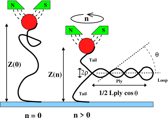
Figure 1: The magnetic tweezer experiment.

When no rotation is put in, the DNA molecule behaves like a semi-flexible polymer, i.e. the relative extension $z$ is a function of the temperature $T$, the persistence length $A$ and the applied pulling force $f$:

$$z(n=0)=1-\left(\frac{4\,k_{B}\,T}{A\,f}\right)^{\frac{1}{2}}.$$ (1)

This relation is used to extract the bending persistence length $A$ from experimental data. Then under gradually increased rotation, the extension $z$ decreases with the number of turns $n$ put in and eventually the molecule starts to wrap around itself. Geometrically speaking, the DNA molecule is coiling around itself in a helical way. Since the molecule is already a double helix, we speak about supercoiling. Each helical wave of the super helix is called a plectoneme. Different attempts has been made to model this experiment, introducing the concepts of wormlike rod chain [4], or torsional directed random walk [5] but without taking into account the possibility of contact, or dealing with the plectonemes in an ad hoc way [6].

Here we present an elastic model that specifically includes the self-contact of the DNA molecule, but does not take into account thermal fluctuations. Our point is that, in the regime where plectonemes are formed, the relevant physical information is already present in our zero-temperature elastic rod model with hard-wall contact. Due to the base pair conformation, it seems natural to consider DNA as an elastic rod with a non-symmetric cross-section (i.e. two different bending rigidities). Nevertheless it has been shown that when dealing with a long enough molecule (more than a few dozen base pairs), one could simplify the model and work with an effective rod having a symmetric cross-section (i.e. one bending rigidity that is the harmonic mean of the two raw rigidities) [7]. In order to focus on supercoiling, we consider the simplest elastic rod model than includes twist effects and can have 3D shapes. Following the classic terminology of Euler planar elastica for twistless 2D shapes, we call the present model the Kirhhoff ideal elastica [8]. The elastic energy reads:

$$E=\frac{1}{2}\,\int_{0}^{L}\left(K_{0}\,\kappa^{2}(s)+K_{3}\,\tau^{2}(s)\right)ds$$

where $s$ is the arc-length, $\kappa(s)$ the curvature of the centre line, $\tau(s)$ the twist rate of the cross section around the centre line (which in the case of an ideal elastica is a constant of $s$), and $K_{0}$ and $K_{3}$ are the bending and twist rigidities respectively. The Kirchhoff equilibrium equations read:

$$\mbox{\boldmath$F$}^{\prime}(s)+\mbox{\boldmath$p$}(s) = 0$$ (2)

$$\mbox{\boldmath$M$}^{\prime}(s)+\mbox{\boldmath$R$}^{\prime}(s)\times\mbox{\boldmath$F$}(s) = 0$$ (3)

where $\mbox{\boldmath$F$}(s)$ and $\mbox{\boldmath$M$}(s)$ are the internal force and moment respectively. The external force per unit length $\mbox{\boldmath$p$}(s)$ can model an electrostatic repulsion, gravity or hard-wall contact. The centre line of the rod is given by $\mbox{\boldmath$R$}(s)$ and $\mbox{\boldmath$t$}(s)=\mbox{\boldmath$R$}^{\prime}(s)$ is its tangent. In the case of an ideal rod it can be shown [9] that:

$$K_{0}\,\mbox{\boldmath$t$}^{\prime}(s) = \mbox{\boldmath$M$}(s)\times\mbox{\boldmath$t$}(s)$$ (4)

$$K_{0}\,\mbox{\boldmath$d_{1}$}^{\prime}(s) = \left(\mbox{\boldmath$M$}(s)-\tau\left(K_{3}-K_{0}\right)\mbox{\boldmath$t$}(s)\right)\times\mbox{\boldmath$d_{1}$}(s)$$ (5)

where $\mbox{\boldmath$d_{1}$}(s)$ is a unit vector, lying in the cross section, that follows the twist of the centre line. For a DNA molecule, it is generally taken as the vector pointing toward the major groove.

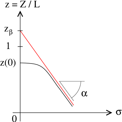
Figure 2: Fitting the linear part of the response curve.

For the parts free of contact, we have $\mbox{\boldmath$p$}(s)\equiv\mbox{\boldmath$0$}$. In case of self-contact there are two points along the rod, say at arclength $s_{1}$ and $s_{2}$, where the inter-strand distance $|\mbox{\boldmath$R$}(s_{1})-\mbox{\boldmath$R$}(s_{2})|$ is equal to twice the radius of the circular cross-section (which we denote by $\rho$). At point $s_{1}$, we introduce a finite jump in the force vector $\mbox{\boldmath$F$}(s)$:

$$\mbox{\boldmath$F$}(s<s_{1})=\mbox{\boldmath$F$}(s>s_{1})+\frac{\Delta F_{12}}{2\rho}\,\left(\mbox{\boldmath$R$}(s_{1})-\mbox{\boldmath$R$}(s_{2})\right)$$ (6)

where $\Delta F_{12}$ is a positive real number. The same treatment is done at point $s_{2}$, with the same $\Delta F_{12}$ [9, 10]. This corresponds to having a Dirac function for $\mbox{\boldmath$p$}(s)$ in (2). In case of continuous sections of contact $\mbox{\boldmath$p$}(s)$ is a function with changing direction and intensity. In our model we only consider cases where the contact occurs either at discrete points or along straight lines. This model has already been used [11, 12] and is well described in [10].

Ideally we are looking for equilibrium configurations of the ideal elastica that match the boundary conditions corresponding to the magnetic tweezer experiment. Nevertheless, in case of a long rod ($L\gg\rho$) with a large number of turns $n$ put in, the exact geometry of the boundary conditions are less important, and we choose clamped ends as used before [9]. We numerically find equilibrium configurations matching the boundary conditions using classical path following techniques; first a self made algorithm relying on multiple (or parallel) shooting, then using the code AUTO [13] that discretises the boundary value problem with Gauss collocation points. The different types of solutions (straight, buckled, supercoiled) are found in the following way. We fix the radius $\rho$ and the vertical component $f$ of the force vector $\mbox{\boldmath$F$}(s=0)$ acting on the bead. We first consider a straight rod with no rotation $n=0$. Then we twist the rod by gradually increasing $n$. At a certain bifurcation value, the path of straight solutions crosses another path of buckled solutions. Following this new path, we end up crossing another path of solutions with one discrete contact point. This latter path will itself intersect a path of configurations with two contact points. Solutions with up to three discrete contact points have been found [9]. Eventually the configurations with three discrete contact points bifurcate to solutions including a line of contact in addition of discrete contact points. We call them supercoiled configurations. In a supercoiled configuration, the parts of the rod which are in continuous contact have an helical shape. We call this twin super-helix a ply. The super-helix is defined by its radius $\rho$ and its helical angle $\theta$ (see fig. (1)). Each time we change the fixed pulling force $f$ or the radius $\rho$, the entire numerical continuation has to be rerun. Since we do not consider thermal fluctuations, the first part of our numerical response curve does not correspond to what is found experimentally. On the other hand our model reproduces quite precisely the part of the response curve where the distance $z$ decreases linearly with the number of turns $n$, provided we identify $\rho$ not with the crystallographic radius of the DNA molecule but with an effective supercoiling radius due to electrostatic as well as entropic repulsion. We numerically find that in the linear regime the helical angle $\theta$ does not vary with $n$. We fit numerical solutions curves as in [14] and we find that $\theta$ only depends on $f$, $K_{0}$, and $\rho$:

$$f=\frac{K_{0}}{\rho^{2}}\,\phi_{3}(\theta)\mbox{ with }\phi_{3}(\theta)=1.65805\,\theta^{4}\,.$$ (7)

This result enables us to extract the effective supercoiling radius $\rho$ and the twist rigidity $K_{3}$ from magnetic tweezer experiments on DNA. First we note that the number of turns $n$ applied to the magnetic bead can be interpreted as the excess link of the DNA molecule: $n=\Delta Lk$. Link is normally defined for a closed ribbon but carefull use of a closure permits the introduction of the link of an open DNA molecule [15, 16]. We use the Călugăreanu-White-Fuller theorem to decompose the excess link:

$$(n=)\,\Delta Lk=\Delta Tw+Wr$$ (8)

where $\Delta Lk$ (resp. $\Delta Tw$) is the difference between the actual link (resp. twist) and the intrinsic link (resp. twist) of the double helix. The writhe $Wr$ is the average number of crossings of the centre line one sees when looking at the molecule from (all the possible) different viewpoints.

Figure 3: Experimental response curves with a 48kbp DNA molecule in a 10 mM phosphate buffer [3]. Each curve corresponds to an experiment carried at a constant pulling force. Forces are, from bottom to top, 0.25, 0.33, 0.44, 0.57, 0.74, 1.1, 1.31, 2.2, 2.95, 4.15, and 4.9 pN.

In the ply part, the twist rate is related to the helical angle $\theta$ via a mechanical balance [10, 17]:

$$\tau=(-\epsilon)\frac{K_{0}}{2\rho\,K_{3}}\,\left(\tan 2\theta-\sin 2\theta\right)\,,$$ (9)

where $\epsilon=\pm 1$ stands for the chirality of the ply [17]. Since the twist rate is constant along the rod, we have $\Delta Tw=\tau\,L/(2\pi)$. Generally writhe is not additive but using Fuller theorem [18] with a carefully choosen reference curve we may write :

$$Wr=Wr_{loop}+Wr_{tails}+Wr_{ply}.$$ (10)

Here we neglect $Wr_{loop}$ and $Wr_{tails}$. Carefully choosing a reference curve to apply Fuller theorem or directly computing the writhe from the double integral yields [15]:

$$Wr_{ply}=(-\epsilon)\frac{L_{ply}}{4\pi\,\rho}\sin 2\theta\,.$$ (11)

The total contour length (or number of base pairs) $L$ of the DNA molecule is given and we write:

$$L_{ply}=L-L_{loop}-L_{tails}\,.$$ (12)

We neglect $L_{loop}$ and we use an heuristic equation for $L_{tails}$ :

$$L_{tails}=Z(\sigma)\,\frac{L}{Z(0)},$$ (13)

which means that when the molecule is supercoiled the tails parts, which are not supercoiled, are as disordered as the molecule was when no rotation was put in. For positive supercoiling ($n>0$) we get a left handed ply ($\epsilon=-1$). From (8), (9), and (11) we obtain:

$$\Delta Lk=\frac{L}{4\pi\rho}\left[\frac{K_{0}}{K_{3}}\,\left(\tan 2\theta-\sin 2\theta\right)+\sin 2\theta\left(1-\frac{Z}{Z(0)}\right)\right].$$ (14)

Introducing the supercoiling ratio $\sigma=\Delta Lk/Lk_{0}$ and taking $h=10.5$ base pairs per turn and $\delta z=0.34\,nm$ of rise for each base pair, we get an helical pitch for the DNA double helix $H=h\,\delta z=3.57\,nm$ and we have: $Lk_{0}=L/H$. Equation (14) can then be inverted to give an approximation of the linear part of the response curve in the $(\sigma,z)$ plane :

$$\frac{z}{z(0)}=1+\frac{K_{0}}{K_{3}}\left(\frac{1}{\cos 2\theta}-1\right)-\frac{4\pi\rho}{H\sin 2\theta}\,\sigma$$ (15)

$$\begin{array}[]{|c|c|c|c|}\hline\cr f\mbox{ (pN)}&\theta\mbox{ (rad)}&\rho\mbox{(nm)}&K_{3}/K_{0}\\ \hline\cr 0.25&0.427&6.85&1.88\\ 0.33&0.449&6.60&1.87\\ 0.44&0.467&6.17&1.92\\ 0.57&0.469&5.47&1.84\\ 0.74&0.504&5.55&2.01\\ 1.1&0.488&4.26&1.86\\ 1.31&0.471&3.64&1.58\\ 2.2&0.503&3.21&1.65\\ 2.95&0.507&2.81&1.62\\ \hline\cr\end{array}$$

Table 1: Results for the 48kbp DNA molecule in a 10 mM phosphate buffer.

Figure 4: Experimental response curves with a 11kbp DNA molecule in a 150 mM phosphate and 5 mM magnesium (Mg2+) buffer. Forces are, from bottom to top, 0.45, 1.45, and 4.3 pN. Unpublished data from Gilles Charvin.

We use (7) and (15) to extract information from experimental response curves of extension-rotation experiments. Since experiments are carried at given (fixed) $f$ and since $K_{0}$ is obtained from (1) with $K_{0}=A\,k_{B}T$, then from each experimental curve in the $(\sigma,z)$ plane we only need : $(i)$ the relative extension at $\sigma=0$, which we denote by $z(0)$, $(ii)$ the slope of the linear part, which we denote by $\alpha$, $(iii)$ the ordinate at the origin of the straight line fitting the linear part of the response curve, which we denote by $z_{\beta}$. Using (7) and (15) we get an equation for $\theta$ :

$$\alpha=-\frac{4\pi\,z(0)}{H\sin 2\theta}\,\sqrt{\frac{K_{0}}{f}\phi_{3}(\theta)}$$ (16)

Once we know $\theta$, we can extract the effective supercoiling radius $\rho$ from (7) and the effective stifnesses ratio from (15):

$$\frac{K_{3}}{K_{0}}=\left(\frac{1}{\cos 2\theta}-1\right)\Big{/}\left(\frac{z_{\beta}}{z(0)}-1\right)$$ (17)

$$\begin{array}[]{|c|c|c|c|}\hline\cr f\mbox{ (pN)}&\theta\mbox{ (rad)}&\rho\mbox{ (nm)}&K_{3}/K_{0}\\ \hline\cr 0.45&0.307&2.79&1.09\\ 1.45&0.319&1.67&1.00\\ 4.3&0.348&1.15&0.99\\ \hline\cr\end{array}$$

Table 2: Results for the 11kbp DNA molecule in a 150 mM phosphate and 5 mM magnesium (Mg2+) buffer.

Results are shown in table 1 and 2 and can be compared to results of [19] where another micro-technique was used and a value of $K_{3}\simeq 100\,nm\,k_{B}\,T$ (in a 100mM NaCl + 40 mM Tris-HCl buffer) was found. From our results, we see that the effective supercoiling radius decreases with the intensity of the pulling force, and with the strength of the salt buffer. Fitting experimental data with (1) yields $K_{0}=51\,nm\,k_{B}\,T$ for fig. 3 and $K_{0}=57\,nm\,k_{B}\,T$ for fig. 4. This means that the bending rigidity does not vary widely with the salt properties of the buffer. On the other hand, present results imply that the twist rigidity strongly decreases with the salt strength. This in turns implies that the electrostatic contribution (repulsion of the charges lying on the sugar-phosphate backbone) to this effective twist rigidity is rather important.

It is a pleasure to thank G. Charvin, V. Croquette, and D. Bensimon for supplying us with data from experiments.

References

- [1] Stephen R. Quake, Hazen Babcock, and Steven Chu. The dynamics of partially extended single molecules of DNA. Nature, 388:151–154, 1997.
- [2] O. Kratky and G. Porod. Rontgenuntersushung geloster fagenmolekule. Rec. Trav. Chim., 68:1106–1123, 1949.
- [3] T. R. Strick, J.-F. Allemand, D. Bensimon, A. Bensimon, and V. Croquette. The elasticity of a single supercoiled dna molecule. Science, 271:1835–1837, 1996.
- [4] C. Bouchiat and M. Mézard. Elastic rod model of a supercoiled dna molecule. Eur. Phys. J. E., 2:377–402, 2000.
- [5] J. David Moroz and Philip Nelson. Torsional directed walks, entropic elasticity, and dna twist stiffness. PNAS, 94:14418, 1997.
- [6] J. F. Marko and E. D. Siggia. Statistical mechanics of supercoiled dna. Phys. Rev. E, 52(3):2912–2938, 1995.
- [7] S. Kehrbaum and J. H. Maddocks. Effective properties of elastic rods with high intrinsic twist. In Michel Deville and Robert Owens, editors, Proceedings of the 16th IMACS World Congress 2000, 2000. ISBN 3-9522075-1-9.
- [8] Sébastien Neukirch and Michael E. Henderson. Classification of the spatial clamped elastica: symmetries and zoology of solutions. Journal of Elasticity, 68:95–121, 2002.
- [9] G. H. M van der Heijden, S. Neukirch, V. G. A. Goss, and J. M. T. Thompson. Instability and self-contact phenomena in the writhing of clamped rods. Int. J. Mech. Sci., 45:161–196, 2003.
- [10] B. D. Coleman and D. Swigon. Theory of supercoiled elastic rings with self-contact and its application to DNA plasmids. Journal of Elasticity, 60:173–221, 2000.
- [11] D. M. Stump, W. B. Fraser, and K. E. Gates. The writhing of circular cross-section rods: undersea cables to dna supercoils. Proc. R. Soc. Lond. A, 454:2123–2156, 1998.
- [12] Zolt Gáspár and R. Németh. A special shape of a twisted ring. In Proc. of 2nd European Conference on Computational Mechanics, page 11, Cracow, Poland, June 26-29 2001. CD.
- [13] Eusebius Doedel, Herbert B. Keller, and Jean Pierre Kernevez. Numerical analysis and control of bifurcation problems (i) bifurcation in finite dimensions. International Journal of Bifurcation and Chaos, 1(3):493–520, 1991.
- [14] D. M. Stump and W. B. Fraser. Multiple solutions for writhed rods: implications for dna supercoiling. Proc. R. Soc. Lond. A, 456:455–467, 2000.
- [15] E. L. Starostin. On the writhe of non-closed curves. arXiv: physics/0212095, 2002.
- [16] V. Rossetto and A. C. Maggs. Writhing geometry of open dna. The Journal of Chemical Physics, 118(21):9864–9874, 2003.
- [17] Sébastien Neukirch and Gert van der Heijden. Geometry and mechanics of uniform n-plies: from engineering ropes to biological filaments. Journal of Elasticity, 69:41–72, 2002.
- [18] Jürgen Aldinger, Isaac Klapper, and Michael Tabor. Formulae for the calculation and estimation of writhe. Journal of Knot Theory and its Ramifications, 4(3):343–372, 1995.
- [19] Zev Bryant, Michael D. Stone, Jeff Gore, Steven B. Smith, Nicholas R. Cozzarelli, and Carlos Bustamante. Structural transitions and elasticity from torque measurements on dna. Nature, 424:338–341, 2003.