Fluctuation-dissipation theorem and models of learning

Abstract

Advances in statistical learning theory have resulted in a multitude of different designs of learning machines. But which ones are implemented by brains and other biological information processors? We analyze how various abstract Bayesian learners perform on different data and argue that it is difficult to determine which learning–theoretic computation is performed by a particular organism using just its performance in learning a stationary target (learning curve). Basing on the fluctuation–dissipation relation in statistical physics, we then discuss a different experimental setup that might be able to solve the problem.

1 Introduction

Learning based on experience (variously known as sensing, information processing, or adaptation) is ubiquitous on all scales in biology. For example, on the molecular scale, the Lac operon in E. coli learns the lactose concentration to produce $\beta$–galactosidase (the lactose–metabolizing enzyme) in proper quantities (Cohn and Horibata, 1959). Similarly, in the sensory system, the retinal phototransduction cascade uses the information in the arrivals of photons to learn the instantaneous light intensity and thus the current visual scene (Detwiler et al., 2000). Additionally, it also learns the ambient light level (to adapt to it) and the temporal correlations (to estimate motion) (Reichardt, 1961; de Ruyter van Steveninck, Personal communication). On the scale of cellular (neuronal) networks, learning, memory, and adaptation in the neural code are a text book knowledge [see e. g., (Brenner et al., 2000; Fairhall et al., 2001)]. At yet larger scales, experiments on rodents are revealing how they learn and respond to changes in their environments (Gallistel et al., 2001); this is a simple, albeit quantifiable, example of the general phenomenon we call “learning” in everyday life. Finally, we may also view evolution as an example of learning, where entire species adapt to the world by means of natural selection.

The creativity of theorists matches that of the Nature, and the number of various learning paradigms different in their goals, assumptions, methods, and performance guarantees is astonishing—too large to enumerate here. Fortunately, it is possible to build uniform foundations for many of these learning machines (Vapnik, 1998; Nemenman, 2000; Bialek et al., 2001), and to find analogs among, say, Structural Risk Minimization (Vapnik, 1998) and Bayesian (Press, 1989) models. However, while one might argue that biological systems are (efficiently) implementing one of many abstract learning–theoretic computations (Attneave, 1954; Barlow, 1959, 1961; Atick, 1992; Bialek et al., 2001), it is often unclear which exact computation is performed in a particular case. For example, what is a learning–theoretic model equivalent to a rat (Gallistel et al., 2001)? or to a simple neural network that tries to maximize its reward (Seung, 2003)? Answering such questions may explain some of animal behaviors, uncover which assumptions they make about the surrounding world, and establish quantitative limits on their learning performance.

To attack the problem, one can construct a biologically plausible computing machine with a known learning–theoretic equivalent (Rao, 2004) and then search for a structural similarity with a real leaving organism. We do not pursue this approach, but choose a more traditional route to establish the equivalence: comparison of performance of real creatures to that of abstract learning machines. As we will argue, analysis of paradigmatic learning curves is not always easy. Thus one of the most important results of the paper is a suggestion of a new protocol for making such comparisons. The intuition behind the suggestion comes from the famous Fluctuation–Dissipation Theorem (Ma, 1985). Based on this analysis and on plausible assumptions about statistics of natural stimuli, we also suggest that a particular learning–theoretic model might be better suited for biological learning than the alternatives, and thus it should be realized often in reality if optimization of learning is desired.

To follow this route, we need to understand characteristics of learning within different mathematical models fairly well, and a large part of the paper is devoted to this. Analysis is done in the framework of unsupervised Bayesian learning of probability distributions since (a) evidently, Bayesian paradigm is relevant in neuroscience (Kording and Wolpert, 2004), (b) as mentioned, different learning frameworks are often equivalent, and (c) according to Bialek et al. (2001), other learning problems usually can be reduced to unsupervised learning of distributions. Much of this first part of the paper is an abridged review, which follows the spirit and the notation of (Bialek et al., 2001) and often prefers clarity to mathematical rigor. We do not try to make the review self-contained, but instead want to elucidate and emphasize some important points that might have been of a lesser interest in other contexts and also to present some novel results, mostly developed in the Appendices. After these developments, we return to the main question of this work: how can one realistically determine an equivalent learning–theoretic model for a biological organism?

2 The basics of learning

Learning machines should be powerful enough to explain complex phenomena. However, when data is scarce, this power leads to overfitting and poor generalization. Thus a balance must be struck between the abilities to explain and to overfit, and this balance will depend on the amount of data available. In accord, much of statistical learning theory (Jeffreys, 1936; Schwartz, 1978; Janes, 1979; Rissanen, 1989; Clarke and Barron, 1990; MacKay, 1992; Balasubramanian, 1997; Vapnik, 1998; Nemenman, 2000; Bialek et al., 2001) has been devoted to putting the famous paradigm of William of Ockham, Pluralitas non est ponenda sine neccesitate, on firm mathematical footing in various theoretical frameworks. In particular, in Bayesian formulation (Press, 1989; Bernardo, 2003), we know now how proper Bayesian averaging creates Occam factors that punish for complexity and weigh posterior probabilities towards those estimates among a finite set of parametric model families that have the best overall predictive power (Bialek et al., 2001), but do not necessarily produce the best fit to the observed data. This has been called Bayesian model selection.

The waters get murkier in a nonparametric or infinite parameter setting when the whole functional form of an unknown object is to be inferred. Bayesian nonparametric developments generally parallel parametric ones, and techniques of Quantum Field Theory (QFT) help in computations (Bialek et al., 1996; Holy, 1997; Bialek et al., 2001; Cucker and Smale, 2001; Nemenman and Bialek, 2002; Lemm, 2002). However, the exact relationship between the two settings is unknown, and some results suggest subtle logarithmic differences between the cases (Hall and Hannan, 1988; Rissanen et al., 1992; Bialek et al., 2001).

We now review these and other Bayesian learning machines, and we start with an introduction of some important and useful quantities.

Suppose we observe i. i. d. samples $x_{i}$, $i=1\dots N$. For simplicity, we assume that $x$ is a scalar, but this does not affect most of the discussion. We need to estimate the probability density that generates the samples. A priori we know that this density, $Q(x|{\boldsymbol{\alpha}})$, can be indexed by some (possibly infinite dimensional) vector of parameters ${\boldsymbol{\alpha}}$, and the probability of each parameter value is ${\mathcal{P}}({\boldsymbol{\alpha}})$. Then we define the density of models (solutions), at a given distance (dissimilarity, or divergence) $D(\bar{\boldsymbol{\alpha}},{\boldsymbol{\alpha}})=\epsilon$ away from the unknown true target $\bar{\boldsymbol{\alpha}}$, which is being learned:

$$\rho(\epsilon;\bar{\boldsymbol{\alpha}})=\int d{\boldsymbol{\alpha}}\,{\mathcal{P}}({\boldsymbol{\alpha}})\,\delta\left[D(\bar{\boldsymbol{\alpha}},{\boldsymbol{\alpha}})-\epsilon\right]\,.$$ (1)

For Bayesian inference of probability densities, the correct measure of dissimilarity is the Kullback–Leibler divergence, $D_{\rm KL}(\bar{\boldsymbol{\alpha}}||{\boldsymbol{\alpha}})=\int dx\,Q(x|\bar{\boldsymbol{\alpha}})\log[Q(x|\bar{\boldsymbol{\alpha}})/Q(x|{\boldsymbol{\alpha}})]$ (Bialek et al., 2001), which has an important information–theoretic interpretation (Cover and Thomas, 1991). However, in other situations different choices of $D$ can and should be made.

Performance of a Bayesian learner is usually measured by the speed with which the posterior probability concentrates for $N\to\infty$ (the learning curve) and by whether the point of concentration is the true unknown target (consistency). These characteristics illuminate the importance of $\rho$, as it relates to both of them. First, it has been proven that if, for $\epsilon\to+0$, the density, $\rho(\epsilon;\bar{\boldsymbol{\alpha}})$, is not zero, then the Bayesian problem is consistent (Nemenman, 2000; Bialek et al., 2001). Intuitively, this is because, for large density, statistical fluctuations of the sample and of the estimated parameters result in small $D_{\rm KL}(\bar{\boldsymbol{\alpha}}||{\rm estimate})$, making convergence to the target almost certain.

Relation of $\rho$ to the learning curve is more complicated. We can calculate the average (over samples) Occam factor for a given target (the generalization error, or the fluctuation determinant) to the leading order in $1/N$:

$${\mathcal{D}}(\bar{\boldsymbol{\alpha}};N)\approx-\log\int d\epsilon\,\rho(\epsilon;\bar{\boldsymbol{\alpha}}){\rm e}^{-N\epsilon}\,.$$ (2)

This is the term that emerges as the penalty for complexity in Bayesian model selection (Balasubramanian, 1997; Bialek et al., 2001). If averaged over $\bar{\boldsymbol{\alpha}}$, the Occam factor becomes predictive information (Bialek et al., 2001), which is the average number of bits that $N$ samples provide about the unknown parameters,

$$I_{\rm pred}(N)=\int d\bar{\boldsymbol{\alpha}}\,{\mathcal{P}}(\bar{\boldsymbol{\alpha}}){\mathcal{D}}(\bar{\boldsymbol{\alpha}};N)\,.$$ (3)

Finally, one can define the universal learning curve, which measures the expected $D_{\rm KL}$ between the target and the estimate after $N$ observations (Bialek et al., 2001). Up to the first order in the large parameter $N$, this is

$$\Lambda(\bar{\boldsymbol{\alpha}};N) \approx\frac{d{\mathcal{D}}(\bar{\boldsymbol{\alpha}};N)}{dN}\,,$$ (4)

$$\Lambda(N) =\int d\bar{\boldsymbol{\alpha}}\,{\mathcal{P}}(\bar{\boldsymbol{\alpha}})\Lambda(\bar{\boldsymbol{\alpha}};N)\approx\frac{dI_{\rm pred}}{dN}\,.$$ (5)

Many of these quantities, especially $I_{\rm pred}$, are also natural objects when analyzing complexity of a time series (Bialek et al., 2001).

3 Different models of learning

Since one of the goals of this work is to investigate if learning machines can be discriminated by means of their learning performance, specifically $\Lambda(N)$, here we discuss how $\Lambda$ depends on $N$ for different scenarios.

3.1 Learning in a finite set of parameters

Consider a setup where ${\boldsymbol{\alpha}}$ can take $M$ discrete values $a_{1},a_{2},\dots,a_{M}$ with a priori probabilities ${\mathcal{P}}_{1},{\mathcal{P}}_{2},\dots,{\mathcal{P}}_{M}$, and their divergences from the target $a_{1}$ are $0=d_{1}<d_{2}<\cdots<d_{M}$. The density is $\rho(\epsilon;a_{1})=\sum_{i=1}^{M}{\mathcal{P}}_{i}\delta(d_{i}-\epsilon)$. For $N\to\infty$, we have

$${\mathcal{D}}(a_{1};N) = -\log\sum_{i=1}^{M}{\mathcal{P}}_{i}\exp[-Nd_{i}]\approx-\log{\mathcal{P}}_{1}-{\mathcal{P}}_{2}/{\mathcal{P}}_{1}\exp[-Nd_{2}],$$ (6)

$$\Lambda(a_{1};N) \approx d_{2}{\mathcal{P}}_{2}/{\mathcal{P}}_{1}\exp[-Nd_{2}].$$ (7)

So exponential learning curves (and asymptotically finite ${\mathcal{D}}$ and $I_{\rm pred}$) correspond to learning a possibility in a finite set. Similarly, we can construct models with $\Lambda(N)\propto 1/N^{\nu},\nu>1$, and they will also have asymptotically finite $I_{\rm pred}$.

3.2 Finite parameter learning

Now let the target probability density $Q(x|\bar{\boldsymbol{\alpha}})$, or a model, belong to a set of densities $A$, a model family, that can be indexed by a vector of parameters ${\boldsymbol{\alpha}}\in A$, $\dim{\boldsymbol{\alpha}}=K<\infty$, and $\forall{\boldsymbol{\alpha}}\in A,\,{\mathcal{P}}({\boldsymbol{\alpha}})>0$. Then if $A$ is not compact, or if the KL divergence between $\bar{\boldsymbol{\alpha}}$ and the boundary of $A$ is larger than $\epsilon$, then the density of solutions for such $K$–parametric family is (Bialek et al., 2001)

$$\rho(\epsilon;\bar{\boldsymbol{\alpha}})\approx{\cal P}(\bar{\boldsymbol{\alpha}}|r)\frac{2\pi^{K/2}}{\Gamma(K/2)}\frac{\epsilon^{(K-2)/2}}{\sqrt{\det{\mathcal{F}}_{K}}}\,,$$ (8)

where

$${\mathcal{F}}^{\mu\nu}_{K}(\bar{\boldsymbol{\alpha}})=\left.\frac{\partial^{2}D_{\rm KL}(\bar{\boldsymbol{\alpha}}||{\boldsymbol{\alpha}})}{\partial\alpha_{\mu}\partial\alpha_{\nu}}\right|_{{{\boldsymbol{\alpha}}}={\bar{\boldsymbol{\alpha}}}}\,.$$ (9)

$N{\mathcal{F}}_{K}$ is the Fisher information matrix (Cover and Thomas, 1991); its eigenvectors are the principal axes of the error ellipsoid in the parameter space, and the (inverse) eigenvalues are variances of parameter estimates along each of these directions. The prefactor $2\pi^{K/2}/\Gamma(K/2)$ is the area of the $K$–sphere, and it has to be multiplied by the fraction of the sphere that is inside $A$ if the latter is (semi)compact. Eq. (8) now gives

$$I_{\rm pred}(N) \approx {\mathcal{D}}(\bar{\boldsymbol{\alpha}},N)\approx K/2\log N,$$ (10)

$$\Lambda(N) \approx \Lambda(\bar{\boldsymbol{\alpha}},N)\approx K/(2N).$$ (11)

The situation changes slightly if $\bar{Q}\not\in A$ (here $\bar{Q}$ is the target density), and the prior assumptions about the world are wrong. Then we find the best approximation to the target within $A$, $\hat{\boldsymbol{\alpha}}=\arg\min_{\alpha\in A}D_{\rm KL}(\bar{Q}||{\boldsymbol{\alpha}})$, and define the distance between $\bar{Q}$ and $A$, $D_{A}(\bar{Q})\equiv D_{\rm KL}(\bar{Q}||\hat{\boldsymbol{\alpha}})$ [this is similar to the I-projection (Csiszar, 1975), but the order of arguments in $D_{\rm KL}$ is different]. In this case, the model density is zero for $\epsilon\leq D_{A}(\bar{Q})$, and the estimate concentrates near $\hat{\boldsymbol{\alpha}}$ as $N\to\infty$. Thus, if the radius of curvature of $A$ is much larger than $\epsilon$, and $D_{A}(\bar{Q})$ is also small, then Eqs. (8, 11) generalize to

$$\rho(\epsilon;\bar{\boldsymbol{\alpha}}) \approx \left\{\begin{array}[]{l}{\cal P}(\hat{\boldsymbol{\alpha}})\frac{2\pi^{K/2}}{\Gamma[K/2]}\frac{[\epsilon-D_{A}(\bar{Q})]^{(K-2)/2}}{\sqrt{\det{\mathcal{F}}_{K}}},\;\epsilon>D_{A}(\bar{Q}),\\ 0,\;\epsilon\leq D_{A},\end{array}\right.$$ (14)

$$\Lambda(\bar{Q},N) \approx D_{A}(\bar{Q})+K/(2N).$$ (15)

3.3 Nested finite parameter models

Suppose now the target $\bar{Q}(x)$ that generates the observations belongs to one of $R$ model families, $A_{r},r=1\dots R$, with ${\rm Prob}(\bar{Q}\in A_{r})={\mathcal{P}}(r)$. Models in each of the families are indexed by parameters ${\boldsymbol{\alpha}}^{(r)}$, $\dim{\boldsymbol{\alpha}}^{(r)}=K(r)<\infty$, so that the density of observing $x$ in a given model is $Q_{r}(x|{\boldsymbol{\alpha}}^{(r)})$. Within each family, the parameters are a priori distributed according to ${\mathcal{P}}({\boldsymbol{\alpha}}^{(r)}|r)$.

We will assume that the families are nested. By this we mean that $Q_{r}(x|{\boldsymbol{\alpha}}^{(r)})\equiv Q(x|{\boldsymbol{\alpha}})$ are independent of $r$, but that in each family the values of $\alpha_{\mu}$, $\mu>K(r)$, are identically zero. Further, the nonzero parameters have the same a priori distributions in all families:

$${\mathcal{P}}(\alpha_{\mu}|r) = \left\{\begin{array}[]{cc}p(\alpha_{\mu})\,,&\mu\leq K(r)\\ \delta(\alpha_{\mu})\,,&\mu>K(r)\end{array}\right.$$ (18)

$${\mathcal{P}}({\boldsymbol{\alpha}}|r) = \prod_{\mu=1}^{R}{\mathcal{P}}(\alpha_{\mu}|r)$$ (19)

Thus a parameter $\alpha_{\mu}$ is “switched on” (or “activated”) when $r$ reaches $r_{\mu}\equiv\min_{r}\{r:K(r)\geq\mu\}$. Discussion of such nested models has been current in Bayesian (Bernardo, 2003; Raftery and Zheng, 2003) and frequentist (Neter et al., 1996) literature for many years. However, we are unaware of any comprehensive analysis relevant to important questions analyzed in our current presentation, such as those in Appendices A–C.

If $R\to\infty$, then we require that the union of all families forms a complete set, so that every sufficiently smooth probability density can be approximated arbitrarily closely by some member of the union (if needed, this definition can be made more precise).

For simplicity, in this paper we focus on

$$p(\alpha_{\mu}) ={\mathcal{N}}(0,\sigma_{\mu}^{2})\,,$$ (20)

$$\sigma_{\mu} =cr_{\mu}^{-\beta},\,\beta\geq 0,\,c={\rm const}\,,$$ (21)

where ${\mathcal{N}}(a,b)$ denotes a normal distribution with the mean of $a$ and the variance of $b$. In particular, $\beta=0$ corresponds to the same in–family a priori variances for all active parameters. This is common when discussing Bayesian model selection.

While these priors describe a set of parametric models, another view is also possible. The joint distribution of $r$, ${\boldsymbol{\alpha}}$, and $\{x\}$ is $P(\{x\},{\boldsymbol{\alpha}},r)=Q(\{x\}|{\boldsymbol{\alpha}}){\mathcal{P}}({\boldsymbol{\alpha}}|r){\mathcal{P}}(r)$, which results in

$$P(\{x\},{\boldsymbol{\alpha}}) = \sum_{r}Q(\{x\}|{\boldsymbol{\alpha}}){\mathcal{P}}({\boldsymbol{\alpha}}|r){\mathcal{P}}(r)=Q(\{x\}|{\boldsymbol{\alpha}})\sum_{r}{\mathcal{P}}({\boldsymbol{\alpha}}|r){\mathcal{P}}(r)$$ (22)

$$\equiv Q(\{x\}|{\boldsymbol{\alpha}}){\mathcal{P}}({\boldsymbol{\alpha}})\,,$$

where the last equation defines ${\mathcal{P}}({\boldsymbol{\alpha}})$, the overall prior over ${\boldsymbol{\alpha}}$. Unlike ${\mathcal{P}}({\boldsymbol{\alpha}}|r)$, ${\mathcal{P}}({\boldsymbol{\alpha}})$ is not factorizable and is not differentiable at zero for any $\alpha_{\mu}$, $\mu>K(1)$. Thus the nested setup may be viewed as inference in a combined model family with $K(R)$ parameters. In particular, for $R$ and $K(R)\to\infty$, the learning problem has a countable infinity of parameters leading to the common assumption of equivalence with the nonparametric inference.

It is of interest to calculate the combined a priori mean and variance of ${\boldsymbol{\alpha}}$. Integrating over all $\alpha_{\nu}$, $\nu\neq\mu$, we get the combined prior for $\alpha_{\mu}$

$${\mathcal{P}}(\alpha_{\mu})=\delta(\alpha_{\mu})\sum_{r<r_{\mu}}{\mathcal{P}}(r)+p(\alpha_{\mu})\sum_{r\geq r_{\mu}}{\mathcal{P}}(r)\,.$$ (23)

By Eq. (20), the a priori means of all parameters are zero, and the variances are

$$\langle\delta\alpha^{2}_{\mu}\rangle=\sigma^{2}_{\mu}\sum_{r\geq r_{\mu}}{\mathcal{P}}(r).$$ (24)

Thus the bare variance $\sigma^{2}_{\mu}$ is “renormalized” by the probability to be in a family, in which the parameter is nonzero. An interesting special case is

$${\mathcal{P}}(r) \propto r^{-\gamma}\,,\quad\gamma>1,\;\;R\to\infty,$$ (25)

$$r_{\mu} = \mu\,.$$ (26)

Then the a priori variance gets a simple form

$$\langle\delta\alpha^{2}_{\mu}\rangle\propto\mu^{-\beta}\sum_{r=\mu}^{\infty}r^{-\gamma}\sim\mu^{-\beta-\gamma+1}\,.$$ (27)

Thus $\langle\delta\alpha_{\mu}^{2}\rangle$ depends as much on the bare variance as on the speed of decay of ${\mathcal{P}}(r_{\mu})$. This suggests that the learning properties of the nested setup will depend equivalently on $\beta$ and $\gamma$. In fact, as shown in Appendix A, this is not true: while behavior of $p(\alpha_{\mu})$ is important, any reasonable choice of ${\mathcal{P}}(r)$ does not effect success of the learning.

From Eq. (14) we can now evaluate the model density and the learning curve for the nested setup. For each value of $\bar{\boldsymbol{\alpha}}$ and $r$, we can find the model $\hat{\boldsymbol{\alpha}}_{r}=\arg\min_{\alpha\in A_{r}}D_{\rm KL}(\bar{\boldsymbol{\alpha}}||{\boldsymbol{\alpha}})$ that best approximates $\bar{\boldsymbol{\alpha}}$ in $A_{r}$, and define $D_{r}(\bar{\boldsymbol{\alpha}})\equiv D_{\rm KL}(\bar{\boldsymbol{\alpha}}||\hat{\boldsymbol{\alpha}})$, the distance between $\bar{\boldsymbol{\alpha}}$ and $A_{r}$. If $\bar{\boldsymbol{\alpha}}\in A_{r}$, then $\bar{\boldsymbol{\alpha}}=\hat{\boldsymbol{\alpha}}$, and $D_{r}(\bar{\boldsymbol{\alpha}})=0$. However, if $\bar{\boldsymbol{\alpha}}\not\in A_{r}$, then $D_{r}(\bar{\boldsymbol{\alpha}})>0$. We then have:

$$\rho(\epsilon;\bar{\boldsymbol{\alpha}})=\sum_{r:\,D_{r}(\bar{\boldsymbol{\alpha}})\leq\epsilon}{\mathcal{P}}(r){\cal P}(\hat{\boldsymbol{\alpha}}_{r}|r)\frac{2\pi^{K(r)/2}}{\Gamma[K(r)/2]}\frac{[\epsilon-D_{r}(\bar{\boldsymbol{\alpha}})]^{[K(r)-2]/2}}{\sqrt{\det{\mathcal{F}}_{K(r)}}}\,.$$ (28)

The learning curve in this scenario strongly depends on the target. Let $\bar{\boldsymbol{\alpha}}$ have $\bar{r}$ active modes (with $\bar{r}$ determined according to ${\mathcal{P}}(\bar{r})$), and let each of these modes have an amplitude $\sim\sigma$ (that is, $\beta=0$). Then $D_{r}(\bar{\boldsymbol{\alpha}})$ is either exactly zero (for $r\geq\bar{r}$), or large (for $r<\bar{r}$). So Eq. (28) becomes

$$\rho(\epsilon\to 0;\bar{\boldsymbol{\alpha}}_{{\rm typ};\bar{r}})\sim\sum_{r\geq\bar{r}}{\mathcal{P}}(r){\cal P}(\hat{\boldsymbol{\alpha}}_{r}|r)\frac{2\pi^{K(r)/2}}{\Gamma[K(r)/2]}\frac{\epsilon^{[K(r)-1]/2}}{\sqrt{\det{\mathcal{F}}_{K(r)}}},$$ (29)

where $\bar{\boldsymbol{\alpha}}_{{\rm typ};\bar{r}}$ is a distribution typical in $A_{\bar{r}}$. This is dominated by $r=\bar{r}$, and for $N\gg K(\bar{r})$ the learning curve is

$$\Lambda(N)\approx\frac{K(\bar{r})}{2N}.$$ (30)

It is now clear that averaging over ${\mathcal{P}}(\bar{r})$ is not very informative. Note also that, for $N\lesssim\bar{r}$, the learning curve goes through a cascade of $K(r)/N$ behaviors, $1\leq r\leq\bar{r}$, and changes of the prefactor of the $N^{-1}$ scaling correspond to activations of new parameters, which happen rather abruptly (cf. Appendix A).

3.4 Nonparametric learning

Nonparametric learning usually refers to inferring a functional form of a probability density $Q(x)$, or rather of $\phi(x)\equiv-\log Q(x)$, with some smoothness constraints on it. The constraints may be in the form of bounding some derivatives of $Q$ or $\phi$, which was the choice of Hall and Hannan (1988) and Rissanen et al. (1992). Alternatively, in the Bayesian framework followed here, the constraints may be incorporated into a functional prior that makes sense as a continuous theory, independent of discretization of $x$ on small scales. For $x$ in one dimension, the minimal and the most common choice is (Bialek et al., 1996; Aida, 1999; Nemenman and Bialek, 2002; Lemm, 2002)

$${\cal P}[\phi(x)]=\frac{1}{{\mathcal{Z}}}\exp\left[-\frac{\ell^{2\eta-1}}{2}\int dx\left(\frac{\partial^{\eta}\phi}{\partial x^{\eta}}\right)^{2}\right]\,\delta\left[\frac{1}{l_{0}}\int dx\,{\rm e}^{-\phi(x)}-1\right],$$ (31)

where $\eta>1/2$, ${\mathcal{Z}}$ is the normalization constant, and the $\delta$-function enforces normalization of $Q$. The hyperparameters $\ell$ and $\eta$ are called the smoothness scale and the smoothness exponent, respectively. Fractional order derivatives are defined by multiplying by the wave number to the appropriate power in the Fourier representation of $\phi$ (we assume periodicity on $[0,1)$).

This prior is equivalent to specifying a 1–dimensional Quantum Field Theory (Bialek et al., 1996; Holy, 1997; Nemenman and Bialek, 2002; Lemm, 2002), and QFT methods have been successful in the analysis. In particular, the maximum likelihood estimate of the distribution, $Q^{*}(x)\equiv\exp[-\phi^{*}(x)]$, is given by the following differential equation

$$\ell^{2\eta-1}{\mathbb{R}}_{-2\eta}\frac{\partial^{2\eta}\phi^{*}(x)}{\partial x^{2\eta}}-NQ^{*}(x)+\sum_{i}\delta(x-x_{i})=0\,,$$ (32)

where the operator ${\mathbb{R}}_{\theta}$ shifts the phase of each Fourier component of its argument by $\pi\theta/2$ . The equation shows that derivatives of $\phi^{*}$ and $Q^{*}$ of order $2\eta-1$ have step discontinuities. Thus, for $2\eta=1$ the classical solution itself, $\phi^{*}(x)$, is discontinuous, and for $2\eta<1$ the singularities are even more severe. We may characterize sample–dependent fluctuations in $Q^{*}$ by $D_{\rm KL}=\int dx\,Q^{*}_{1}(x)\log Q^{*}_{1}(x)/Q^{*}_{2}(x)$, where $Q^{*}_{1}$ and $Q^{*}_{2}$ are saddle point solutions for different sample realizations. If $Q^{*}$ has, at least, step discontinuities at the sample points, and these points are random, then $D_{\rm KL}$ does not fall to zero as $N$ grows. Therefore, the QFT setup becomes inconsistent at $\eta=1/2$, even though Bayesian formulation is proper, and the prior can still be normalized by, for example, going to the Fourier representation. This is in contrast to the nested setup, where normalizable priors guarantee consistency.

Bialek et al. (1996, 2001) have calculated the $\epsilon\to 0$ model density and the fluctuation determinant for different $\eta$’s. By noticing from Eq. (32) that $N$ and $\ell$ can enter the solutions only in a combination $N/\ell^{2\eta-1}$, we extend their results and recover correct dependence not only on $\eta$ (for $\eta>1/2$), but also on $\ell$:

$$\rho(\epsilon;\bar{\phi}) \approx A[\bar{\phi}]\,\epsilon^{\xi}\exp\left[-\frac{B[\bar{\phi}]}{\ell\epsilon^{1/(2\eta-1)}}\right],$$ (33)

$${\mathcal{D}}(\bar{\phi};N) \approx C[\bar{\phi}]\,\left(\frac{N}{\ell^{2\eta-1}}\right)^{1/2\eta},$$ (34)

$$\Lambda(\bar{\phi},N) \approx \frac{C[\bar{\phi}]}{2\eta\,\ell^{2\eta-1}}\left(\frac{N}{\ell^{2\eta-1}}\right)^{1/2\eta-1}.$$ (35)

Here $\xi$ depends only on $\eta$, and $A$, $B$, and $C$ are some known related functionals that do not depend on $\ell$. These asymptotics kick in when $N\gg 1/\ell$. In particular, for smaller $N$, $\Lambda\sim 1$ and is barely decreasing. The dependence of $C[\bar{\phi}]$ on $\bar{\phi}$ may be significant (and, possibly, diverging for ill-behaved targets). However, from Eq. (33), the dependence on $\eta$ near $2\eta-1\to+0$ is easier to analyze:

$$C[\bar{\phi}]\sim(2\eta-1)^{1/2\eta-1}\,$$ (36)

with an undetermined value at $2\eta=1$. So for $\eta\to 1/2$, ${\mathcal{D}}$ approaches extensivity in $N$, and then becomes ill-defined, again signaling inconsistency. As discussed by Bialek et al. (2001), problems with ${\mathcal{D}}(N)/N\to{\rm const}$ are the most complicated correctly posed learning problems that exist, and they can be studied in the Bayesian QFT setting.

For comparison with the nested case (cf. Appendix B), we may replace $\phi$ by its Fourier series,

$$\phi(x|{\boldsymbol{\alpha}}) \equiv -\log Q(x|{\boldsymbol{\alpha}})=\alpha_{0}+\sum_{\mu=1}^{r}\left(\alpha_{\mu}^{+}\cos 2\pi\mu x+\alpha_{\mu}^{-}\sin 2\pi\mu x\right),$$ (37)

$$\alpha_{0} = \log\int dx\,\exp\left[-\sum_{\mu=1}^{r}\left(\alpha_{\mu}^{+}\cos 2\pi\mu x+\alpha_{\mu}^{-}\sin 2\pi\mu x\right)\right]\,,$$ (38)

with $r\to\infty$ (finite $r$ results in a finite parameter model). The last equation enforces normalization, $\int dx\,Q(x|{\boldsymbol{\alpha}})=1$, and it is equivalent to the constraint $\delta\big{(}\int\exp[-\phi(x|{\boldsymbol{\alpha}})]dx-1\big{)}$ in the prior ${\mathcal{P}}({\boldsymbol{\alpha}}|r)$ or ${\mathcal{P}}[\phi(x)]$. Since the Jacobian of the transformation $\phi(x)\to\{\alpha^{\pm}_{\mu}\}$ is a constant, Eq. (31) amounts to zero-mean Gaussian priors over $\alpha_{\mu}^{\pm}$ with the variance (Nemenman and Bialek, 2002)

$$\langle(\delta\alpha_{\mu}^{\pm})^{2}\rangle=\frac{2}{\ell^{2\eta-1}}\frac{1}{\left(2\pi\mu\right)^{2\eta}},\quad\quad\mu>0.$$ (39)

Equations (27, 39) suggest that the nested and nonparameteric case are similar: the a priori means of the amplitudes are zero, and the variances fall off as power laws in $\mu$. However, the field theory model requires the variance to decrease at least as fast as $1/\mu$ (recall that $\eta>1/2$), while the finite parameter case does not impose such constraints. This is an indication of an essential difference between the models: in the nested case, the priors, specifically the a priori variances of parameters, have less of an influence on learning. This can be easily explained. QFT nonparametric models do not have a sharp separation between active and passive modes. The modes with low $\mu$ are determined by the data, but fluctuations for larger $\mu$ are inhibited only due to the small a priori variances, Eq. (39). The exact attenuation of the fluctuation depends on the values of $\eta$ and $\ell$, and the cumulative contribution to posterior variance of the estimator may be substantial. In contrast, for the finite parameter nested case, once the most probable model family is determined, fluctuations of the higher order parameters are inhibited exponentially (cf. Appendix A). The cumulative fluctuations are then small and almost independent of the a priori parameter variances, and the learning may succeed even for ${\mathcal{P}}(r)$ with a long tail.

The dependence of the QFT model on the prior can be weakened by treating $\ell$ as an unknown random variable and averaging over it (Bialek et al., 1996; Nemenman and Bialek, 2002) (similar averaging over $\eta$ has not yet been performed). This is akin to nesting of finite dimensional models and improves learning curves for a wide range of targets. On the other hand, integration over $\ell$ produces the theory that is not necessarily local in $\phi(x)$, couples all of the Fourier amplitudes, and is difficult to compare to the nested finite parameter setup directly. Therefore, we do not discuss the averaging in what follows, but assume that the values of $\eta$ and $\ell$ used for learning are the best for a particular target being learned.

3.5 Comparing the performance

One of the goals of the paper is to decide if learning curves can be used to distinguish which learning machine is a good description of a particular biological system. To this extent, we need to analyze responses of various learners to data that they are not expecting. Thus in this section we derive learning curves for a finite parameter, a nested ($\beta=0$), and a QFT machine on data that is typical in the prior of one of the two others. With mismatched data and expectations, the learning curve can not be optimal, but may come quite close.

First, consider $\bar{Q}$ taken from the QFT prior. The learning curve for the finite parameter model is given by Eq. (15)—a $N^{-1}$ decay towards some approximate target. Further, as shown in Appendix C, the learning curves for complete nested models, Eq. (75), and for the QFT machine, Eq. (35), which is the best possible machine for such data, differ only logarithmically.

If instead we study a distribution that is typical in the nested case for some $\bar{r}$ (equivalently, a finite parameter distribution with $K(\bar{r})$ parameters) then a finite parameter model again gives Eq. (15). On the other hand, for $N\lesssim K(\bar{r})$, no complete learning machine can estimate all required unknown parameters, and $\Lambda$ does not have a well defined scaling (Nemenman and Bialek, 2002). The differences between the machines emerge for $N\gg\bar{r}$. The nested machine eventually asymptotes to Eq. (30), and starts learning at the rate of $1/N$. However, the QFT setup performs differently: when $\Lambda\to 0$ and all $\bar{r}$ modes are well approximated, the machine continues trying to fit higher order modes, which it expects to be present even though they are not. This will result in the same fluctuation determinant as in Eq. (34), switching to the usual asymptotic $\Lambda\propto(N\ell)^{1/2\eta-1}$ instead of

So, surprisingly, when the target has a finite number of degrees of freedom, the nested setup is qualitatively faster than the QFT learning machine!

4 Learning a changing target

One never needs to know the distribution that generated the data to an infinite precision, and some $\epsilon>0$ approximation is usually enough. Further, if learning in biological systems is stochastic, as argued, for example, by Seung (2003), then $\epsilon$ is bounded from below by the noise variance. As shown by Fairhall et al. (2001) and especially by Gallistel et al. (2001), convergence to the “good enough” estimate happens so quickly, that the transient learning curves are difficult to resolve. Is then the performance difference between the nested and the QFT scenarios seen in the previous section important? And can it be used to discriminate between the models?

4.1 Model density and variable stimuli

Notice that often the target itself changes while being learned. The ambient light intensity may be fluctuating while our eye estimates it, or the variance of angular velocities measured by a fly motion sensitive neuron can be varied by an experimenter while the fly tries to adapt to it (Fairhall et al., 2001). In these cases one has to learn constantly to stay at the allowed $\epsilon$–error, and then a faster learning machine may be truly advantageous. However, even for a variable target, the nested learner will not be helpful if (a) a small change of the target parameters throws it back to a very large $\Lambda$, or (b) the changing target may drift to a region where $\bar{r}$ is so large that the nested setup is not better than the nonparametric anymore.

To answer these concerns, instead of focusing on the density of solutions as a function of the allowed error $\epsilon$, we will keep $\epsilon$ fixed and vary $\bar{\boldsymbol{\alpha}}$. For some small $\epsilon$, a schematic drawing of dependence of $\rho$ on $\bar{\alpha}^{+}_{1}$ and $\bar{\alpha}^{+}_{2}$ with the other parameters fixed at 0 is shown on Fig. 1. In the nested case, there is a ridge along $\alpha^{+}_{2}\approx 0$, where the density is, at least, $\sim 1/\sqrt{\epsilon}$ larger than anywhere else, cf. Eq. (28). The ridge comes from the prior, Eq. (22), for $\bar{\alpha}^{+}_{2}=0$ being singularly larger than for $\bar{\alpha}^{+}_{2}\neq 0$, and the singularity is then smoothed out by $\epsilon$–approximation. In comparison, the nonparametric prior has a bivariate normal shape, which after $\epsilon$–smearing results in a weak target dependency of $\epsilon$–independent prefactors in Eq. (33); thus $\rho(\bar{\boldsymbol{\alpha}})$ varies slowly.

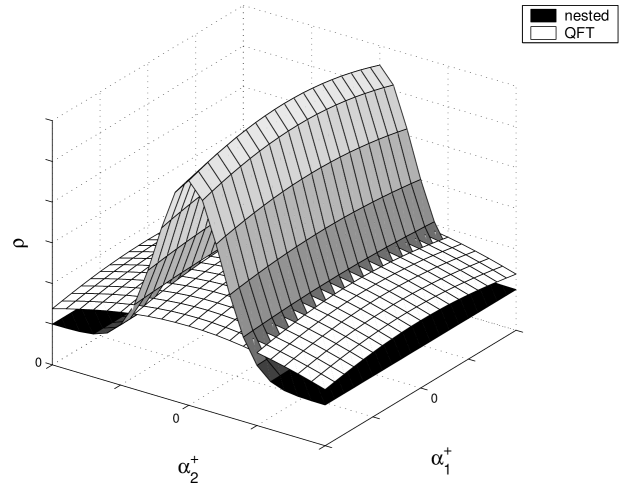
Figure 1: Schematic density of models as a function of the target location.

Figure 1 answers both of the concerns mentioned above. For a QFT machine, densities everywhere are comparatively small. So a small change of the target means vast and slow relearning. In contrast, if, for a nested case, $\bar{\boldsymbol{\alpha}}$ is in the large density region, then there are many other models in the vicinity. Small parameter changes likely leave the target close, and not much needs to be relearned. Further, since the ridge drops off smoothly, models in the vicinity of a large density target also have large densities, and thus are learned fast as well. Of course, this holds only when the target, indeed, varies mostly along a small set of directions, and density ridges are aligned with those. Importantly, since at a finite $\epsilon$ the ridge has a finite width, a perfect alignment is not necessary.

We believe that many natural signals have such structure. For example, in phototransduction, instantaneous intensity is determined by the statistics of reflectivities of objects that come in the view and by the mean ambient light intensity. The statistics barely change over long time scales, while the mean intensity depends on, for example, clouds shading the sun and varies a lot and rapidly. The photoreceptor may want to adapt to intricate details of the distribution of reflectivities, but only after it accurately learns the mean light level. A similar separation of time scales is observed in transcriptional regulation, where, for example, changes in the lactose concentration happen on the scale of minutes, while statistics of lactose bursts depends on the environment and is constant for generations. In neuroscience, when estimating an angular velocity, a fly takes into the account the preceding velocity variance (Fairhall et al., 2001), but it may not have time for reaction to higher order moments. Thus we believe that many natural learners that have a need to learn fast, but also to be able to learn a very wide class of models accurately on longer time scales, will be organized as nested learning machines with the density ridges approximately adjusted to fast variable directions.

4.2 Fluctuation-dissipation and determining the model

The prediction in the last Section brings us back to the main question of this work: how can an underlying learning–theoretic computation be inferred? For many reasons, analysis of learning curves is not always a good idea. First, learning may happen so fast that resolving it might present a problem (Gallistel et al., 2001). Second, to estimate $\Lambda(N)$ reliably, we need to average, and a complete instance of the learning curve is just one sample. Such averaging may require prohibitively long experiments. Third, it is well know that animals adapt. Thus eliciting the same response to the same target requires large inter–trial time delays, further increasing the experimental duration. These problems can be traced to learning being an inherently transient behavior, and they might become less severe if we can characterize learning machines by some stationary response properties. A hint comes from the Fluctuation–Dissipation Theorem in statistical physics (Ma, 1985), which states that, if a system fluctuates in the presence of a linear dissipative restoring force, then the variance of fluctuations (a stationary property) is linearly related to the dissipation coefficient (a feature of the transient response). In our case, we may hope that response to a variable target (fluctuations) reveals information about the learning curve (dissipation).

In view of this suggestion, let us now analyze a few examples of a variable target learning. We now denote by ${\boldsymbol{\alpha}}$ an estimate of $\bar{\boldsymbol{\alpha}}$ averaged over many presentations of the same data. We keep almost all parameters fixed (or changing very slowly), while $\bar{\alpha}_{1}(t)$, which is approximately the direction of the ridge in the density of solutions, is allowed to vary. If data are observed for a long time, then $\bar{\alpha}_{\mu}\approx\alpha_{\mu}$ for $\mu\neq 1$ (provided $\bar{\boldsymbol{\alpha}}=\hat{\boldsymbol{\alpha}}$). Now remember that $\Lambda$ is the expected Kullback–Leibler divergence between $\bar{\boldsymbol{\alpha}}$ and ${\boldsymbol{\alpha}}$, which converges to the $\chi^{2}$ distance when it is small. Thus if $\bar{\alpha}_{1}-\alpha_{1}$ is not large,

$$\Lambda\propto(\alpha_{1}-\bar{\alpha}_{1})^{2}.$$ (40)

For a fixed target and $\Lambda\to 0$ (that is, for $N\to\infty$, $\hat{\boldsymbol{\alpha}}=\bar{\boldsymbol{\alpha}}$), all learning curves we studied can be summarized as

$$\frac{\partial\Lambda}{\partial N}=-\zeta_{N}\Lambda^{\nu}.$$ (41)

Here, in particular, $\nu=1$ corresponds to a finite set of solutions along the direction of $\alpha_{1}$, $\nu=2$ is the finite–parameter or nested case, and $\nu=3$ is the $\eta=1$ QFT model. In principle, other values of $\nu\in(0;\infty)$ are possible. The constant $\zeta_{N}\sim 1$ depends on the details of the learning setup. For example, for parametric cases, $\zeta_{N}=2/K(\bar{r})$.

For Eq. (41), which is manifestly true for a fixed $\bar{\boldsymbol{\alpha}}$, to also hold in the fluctuating target case, the learning machine must quickly notice the target’s variation and disregard old samples as soon as they become outdated. Gallistel et al. (2001) show that a rat reacts to changes in the reward rates as fast an ideal detector would. Therefore, this assumption is reasonable for biological systems.

If measurements are taken at a fixed rate, so that $dN/dt={\rm const}$, we can combine Eqs. (40, 41) to get

$$\frac{d\Delta}{dt}=-\zeta\,{\rm sign}(\Delta)\left|\Delta\right|^{2\nu-1}-v_{\bar{\alpha}}\,,$$ (42)

where $\Delta=\alpha_{1}-\bar{\alpha}_{1}$ is the average error of the estimation, $\zeta$ is some unknown constant with the dimensionality of $1/t$ and is basically the scaled sampling rate, and $v_{\bar{\alpha}}$ is the drift velocity of the target. Equation (42) is a clear example of a dissipative system, and it has many analogues in the theories of classical and quantum dissipation (Weiss, 1995). Note also that, unlike in the fluctuation–dissipation analysis in statistical physics, the spectrum of fluctuations, $v_{\bar{\alpha}}$, is not necessarily white and can be controlled by an experimentalist, potentially providing more ways to probe the underlying dissipative dynamics.

If the target’s variation cannot be learned (incomplete or mismatched machine), then Eq. (42) still holds. However, because of Eq. (15), we now have $\Delta=\alpha_{1}-\hat{\alpha}_{1}$ (recall that $\hat{\boldsymbol{\alpha}}$ is the best approximation to the target by a particular learning machine). Thus to trace the evolution of $\alpha_{1}$ using Eq. (42), one would need to evaluate $\hat{\boldsymbol{\alpha}}(\bar{\boldsymbol{\alpha}})$, which can be done from the stationary target analysis. Further, if the target varies along many learnable directions, then for each such direction we have an analog of Eq. (42), possibly with different $\xi$. So the dynamics of $\Lambda$ is still given by Eq. (41) with forcing, but the dissipation constant depends on the number of varying parameters.

Let’s now consider a few different examples of $v_{\bar{\alpha}}$. If $v_{\bar{\alpha}}={\mathcal{A}}$ is a constant, then asymptotically for $t\to\infty$, setting $d\Delta/dt=0$, we find

$$\Delta\to\Delta_{\infty}=-\left(\frac{{\mathcal{A}}}{\zeta}\right)^{1/(2\nu-1)}\,.$$ (43)

The ratio $v_{\bar{\alpha}}/\zeta$ must be $\ll 1$, otherwise $\Delta$ is outside of the $\Lambda\to 0$ asymptotic, for which Eq. (41) is valid. Thus, for small drifts, setups with smaller $\nu$ win qualitatively.

It is also of interest to consider the situation when $\bar{\alpha}_{1}$ undergoes a Brownian motion, $\langle v_{\bar{\alpha}}(t)v_{\bar{\alpha}}(t^{\prime})\rangle=\Omega\,\delta(t-t^{\prime})$. Writing the Fokker-Planck equation for this Langevin dynamics, we easily find the stationary distribution of $\Delta$,

$$P(\Delta)=\frac{\nu}{\Gamma\left(\frac{1}{2\nu}\right)}\left(\frac{\zeta}{\nu\Omega}\right)^{1/(2\nu)}\exp\left\{-\frac{\zeta|\Delta|^{2\nu}}{\nu\Omega}\right\},$$ (44)

which results in the rms fluctuations of

$$\Delta_{\rm rms}=\left\{\nu^{1/\nu}\frac{\Gamma\left(\frac{3}{2\nu}\right)}{\Gamma\left(\frac{1}{2\nu}\right)}\right\}^{1/2}\left(\frac{\Omega}{\zeta}\right)^{1/(2\nu)}.$$ (45)

Again, these results are true only if $\Delta_{\rm rms}\ll 1$, and again smaller $\nu$ provides for better trailing of the target.

Finally, inspired by Fairhall et al. (2001), let’s examine the case of a periodic motion of $\bar{\alpha}_{1}$ and take, for simplicity, $\bar{\alpha}_{1}={\mathcal{A}}\sin\omega t$, and $v_{\bar{\alpha}}={\mathcal{A}}\omega\cos\omega t$. Now Eq. (42) does not have a simple solution. However, we search for an asymptotically periodic $\Delta(t)$ with the same angular frequency of $\omega$. Therefore, if we multiply Eq. (42) by $\cos\omega t$, integrate over a full period, and exchange the order of the differentiation and the integration, we get

$$\frac{d\langle\Delta\,\cos\omega t\rangle}{dt}=-\zeta\langle{\rm sign}(\Delta)\,|\Delta|^{2\nu-1}\cos\omega t\rangle-{\mathcal{A}}\omega\langle\cos^{2}\omega t\rangle,$$ (46)

where $\langle\dots\rangle$ denotes averaging over the period. Since we are looking for stationary oscillations, time derivative applied to any average is zero. This gives

$$\langle{\rm sign}(\Delta)\,|\Delta|^{2\nu-1}\,\cos\omega t\rangle=-\frac{{\mathcal{A}}\omega}{2\zeta}.$$ (47)

Now multiplying Eq. (42) by ${\rm sign}(\Delta)\,\Delta^{2\nu-1}$ and averaging again results in

$$\langle|\Delta|^{4\nu-2}\rangle=\frac{({\mathcal{A}}\omega)^{2}}{2\zeta^{2}},$$ (48)

which is the same scaling as in Eq. (43). However, now we also have a dependence on $\omega$.

There are other cases that can be analyzed, such as a step jump in the target, $\bar{\alpha}_{1}$, its square wave modulation, or its diffusion in a potential (Ornstein–Uhlenbeck process). Interestingly, the last two of these cases were used experimentally by Fairhall et al. (2001). However, we leave the analysis for the future, when it will be answering some specific question and won’t be just a mathematical exercise. Even with the three examples already discussed, it is clear that letting the target move maps the scaling of the learning curve into a stationary property (e. g., variance of the estimation error), which might be easier to analyze experimentally.

5 Discussion

We have shown that, with a moving target, transient learning curves are replaced by different scaling dependences of the estimation errors on the amplitude of the target’s motion. This effect is stationary and may be easier to observe experimentally. However, since we do not have a comprehensive theory of variable target learning yet, a few precautions are in order when designing and analyzing experiments along these lines. (1) Target velocities must be kept small, so that the asymptotic analysis presented in this work holds. (2) The analysis is only valid when the learner forgets past observations as soon as the target changes appreciably. Learning will be much slower if such outdated samples are kept. (3) When varying the stimulus, we have to be reasonably sure that the animal only tracks it, but does not predict it. White noise $v_{\bar{\alpha}}$ or a multiparameter representation of the target in terms of the position, velocity, acceleration, etc., might be a solution. (4) Finally, we have to keep in mind that, in a behaving animal, learning a change in a signal and reacting to it may be separated by a long delay, and special care is needed to observe the former, but not the latter. This being said, it nevertheless is possible that all these and other disadvantages will be outweighed by the ability to determine the correct learning–theoretic model of the organism by varying the amplitude and the nature (say, stochastic or periodic) of the target’s motion and studying typical responses as functions of these parameters.

Consider, for example, the experiment described on Fig. 4 of Fairhall et al. (2001). There the input signal (the standard deviation of the angular velocity, $\sigma(t)$) undergoes a finite variance $\Sigma^{2}$ and a finite correlation time $\tau$ random motion. The instantaneous neuron firing rate $r(t)$ is the estimate of $\sigma(t)$. Repeating exactly the same randomly generated stimulus many times and averaging over spike trains, one may estimate $r(t)$ and, consequently, the rms estimation error $\Delta_{\rm rms}=\langle(\sigma(t)-r(t)^{2}\rangle^{1/2}_{t}$. Studying dependence of $\Delta_{\rm rms}$ on $\Sigma$ and $\tau$ along the lines of Eq. (45), one can estimate $\nu$. Any $\nu\neq 2$ uniquely determines the underlying computational model. For $\nu=2$, to distinguish a usual finite parameter model from the one that is nested, one makes the signal multidimensional (other parameters of the angular velocity, such as the mean and the skewness, vary together with $\sigma$). For, at least, some signal extensions, the nested model will change the magnitude (but not the scaling) of $\Delta_{\rm rms}$ since $\zeta\propto 1/K(\bar{r})$. In contrast, the simpler model will keep the same prefactor but will be converging only to an approximation of the target.

In cognitive experiments of Gallistel et al. (2001), a rat was trying to learn reward rates on different terminals and match its foraging habits correspondingly. It was determined to be an ideal change detector. Now to build a more detailed model of the animal, one can vary the reward rates continuously, repeat experiments many times, and then look at the average mismatch between the stimulus and the response. Then dependence of the mismatch on the parameters of the rate changes will point at a proper class of learning–theoretic models to compare the rat to. Similarly, one can do this type of analysis on artificial neural networks designed explicitly to model particular animal behavior (Seung, 2003); this will build connections between network architectures and types of inference tasks performed by them.

Another conclusion of our work is that the nested setup may learn faster than the QFT one under some conditions. Thus if one desires a complete learning machine, a nested machine should be built unless there is some specific reason to do the opposite (such as knowing that the world is unlikely to have sharp cutoffs). With experiments along the lines suggested above, this prediction should be testable. We should be able to see if our intuitive beliefs about appropriate complexities of learners for particular tasks match the Nature’s choices. It would also be interesting to study if structural characteristics of a learner are correlated with its learning-theoretic description. That is, could it be that modular, irregular networks, like those seen in biochemistry, often compute like parametric or nested machines? And could layered, regular networks in our brains, which are believed to be able to solve the most complicated learning problems, be realizing QFT machines instead?

Appendix A Model family selection in the nested setup

Inference in Bayesian i. i. d. setup is quite standard (Press, 1989; Bialek et al., 1996; Balasubramanian, 1997; Bernardo, 2003; Raftery and Zheng, 2003), and nested case is not very different. For example, a posteriori expectations of parameter values are given by a derivative of the posterior moment generating function (or the partition function), $Z({{\mathbf{J}}})$:

$$\langle\alpha_{\mu}\rangle =\left.\frac{\partial}{\partial J_{\mu}}\right|_{{\bf J}=0}\log Z({\bf J})\,,$$ (49)

$$Z({\bf J}) \equiv\int d{\boldsymbol{\alpha}}\,{\mathcal{P}}({\boldsymbol{\alpha}})\,{\rm e}^{-{\mathcal{L}}({\boldsymbol{\alpha}})+{\bf J}\cdot{\boldsymbol{\alpha}}}\,$$ (50)

$$=\sum_{r}{\mathcal{P}}(r)Z_{r}({\bf J}){r}\,,$$ (51)

$$Z_{r}({\bf J}){r} \equiv\int d^{K(r)}\alpha\,{\rm e}^{-{\mathcal{L}}_{r}({\boldsymbol{\alpha}})+\sum_{\mu=1}^{K(r)}J_{\mu}\alpha_{\mu}}\,,$$ (52)

$${\mathcal{L}}({\boldsymbol{\alpha}}) \equiv\sum_{i=1}^{N}\phi(x_{i}|{\boldsymbol{\alpha}})\,,$$ (53)

$${\mathcal{L}}_{r}({\boldsymbol{\alpha}}) \equiv-\sum_{\mu=1}^{K(r)}\log p(\alpha_{\mu})+\sum_{i=1}^{N}\phi(x_{i}|{\boldsymbol{\alpha}})\,,$$ (54)

$$\phi(x|{\boldsymbol{\alpha}}) \equiv-\log Q(x|{\boldsymbol{\alpha}})\,.$$ (55)

The posterior expectations are thus determined by the properties of the $Z({\bf J})$, which can be calculated using the saddle point analysis for $N\gg 1$. This is difficult for the first form of $Z({\bf J})$, Eq. (50), due to the singularity at $\alpha_{\mu}=0$ [the singularity was also the reason why we left ${\mathcal{P}}({\boldsymbol{\alpha}})$ out of the combined Lagrangian, Eq. (53)]. Hence we return to the nested form, Eq. (51, 52), but the equivalence between the representation should be kept in mind. Exchanging the order of integration and summation in Eqs. (50, 51) and similar is possible if the priors decay sufficiently fast at $r\to\infty$, or are regularized with regularization lifted after averages are calculated. Unless mentioned otherwise, this is always assumed.

The expectation of $\alpha_{\mu}$ in the model families with $K(r)<\mu$ is necessarily zero, and a similar bias towards smaller magnitudes of parameters will be present when we average over families. Therefore, the a priori decrease of the variances with $\mu$, Eqs. (24, 27), will persist a posteriori for finite $N$. This is the famous James and Stein (1961) shrinkage.

The saddle point, also called classical or maximum likelihood, values of parameters in each family, ${\boldsymbol{\alpha}}_{r}^{*}\equiv\{\alpha^{*}_{\mu;r}\}$, and the second derivatives matrix at the saddle, ${\mathbb{F}}_{r}$, are determined by (remember that $\alpha_{\mu;r}^{*}\equiv 0$ for $\mu>K(r)$)

$$\left.\frac{\partial{\mathcal{L}}_{r}({\boldsymbol{\alpha}})}{\partial\alpha_{\mu}}\right|_{{\boldsymbol{\alpha}}={\boldsymbol{\alpha}}_{r}^{*}} =0\,,\;\mu\leq K(r)\,,$$ (56)

$$\left.\frac{\partial^{2}{\mathcal{L}}_{r}({\boldsymbol{\alpha}})}{\partial\alpha_{\mu}\partial\alpha_{\nu}}\right|_{{\boldsymbol{\alpha}}={\boldsymbol{\alpha}}_{r}^{*}} ={\mathbb{F}}_{r}^{\mu\nu}\,,\;\mu,\nu\leq K(r)\,.$$ (57)

To the first order in $1/N$, this gives

$$Z({\bf J})=\sum_{r}{\mathcal{P}}(r)\frac{{\mathcal{P}}({\boldsymbol{\alpha}}_{r}^{*}|r)(2\pi)^{K(r)/2}}{N^{K(r)/2}\det^{1/2}\frac{{\mathbb{F}}_{r}}{N}}Q(\{x\}|{\boldsymbol{\alpha}}_{r}^{*})\,{\rm e}^{\frac{1}{2}{\bf J}_{r}{\mathbb{F}}_{r}^{-1}{\bf J}_{r}+{\bf J}_{r}\cdot{\boldsymbol{\alpha}}_{r}^{*}}\,,$$ (58)

where $\mu\leq K(r)$ components of ${\bf J}_{r}$ are the same as those of ${\bf J}$, and all higher order components are zero. Differentiating, we get:

$$\langle\alpha_{\mu}\rangle=\frac{\sum_{r=1}^{R}\alpha_{\mu;r}^{*}\,{\rm e}^{-{\mathcal{L}}(r)}}{\sum_{r=1}^{R}{\rm e}^{-{\mathcal{L}}(r)}}\,,$$ (59)

$${\mathcal{L}}(r)\equiv-\log{\mathcal{P}}(r)-\sum_{\mu=1}^{K(r)}\log p(\alpha_{\mu;r}^{*})+\sum_{i=1}^{N}\phi(x_{i}|{\boldsymbol{\alpha}}_{r}^{*})+\frac{K(r)}{2}\log\frac{N}{2\pi}+{\rm Tr}\,\log\frac{{\mathbb{F}}_{r}}{N}\,.$$ (60)

For finite $R$, and $\beta=0$, this is the usual Bayesian model family selection: a posteriori expectations are weighted sum over posterior probabilities of families defined by ${\rm e}^{-{\mathcal{L}}(r)}$. This posterior includes the negative maximum likelihood term, $\sum_{i=1}^{N}\phi(x_{i}|{\boldsymbol{\alpha}}_{r}^{*})$, which grows in magnitude linearly with $N$, but decreased as $r$ grows due to nestedness. It also incorporates the fluctuation determinant $\frac{K(r)}{2}\log\frac{N}{2\pi}+{\rm Tr}\,\log\frac{{\mathbb{F}}_{r}}{N}$, which grows logarithmically in $N$, but increases with $r$. Depending on the value of $N$, there will be some $r^{*}$, for which ${\mathcal{L}}(r)$ is minimal. For large $N$, as a discrete analog of the saddle point argument, this value will dominate the sums in Eq. (59), hence some model family will be “selected.”

However, Eqs. (59, 60) become more interesting if one lets $R\to\infty$. The completeness condition ensures that for large enough $r$ one will be overfitting the data, and $Q(x|{\boldsymbol{\alpha}}_{r}^{*})\to 1/N\sum\delta(x-x_{i})$. Therefore, if the sums are dominated by $r\to\infty$, then consistency breaks and the learning fails. One would thus expect two features to influence the success of the learning. First, it is the prior ${\mathcal{P}}(r)$, which switches on extra degrees of freedom: for slowly decaying priors one would expect $r\to\infty$ terms to win. Second, it is the dependence of the likelihood term on $r$, which measures how capable are the newly activated degrees of freedom of overfitting, or, equivalently, how fast $\max_{i}Q(x_{i}|{\boldsymbol{\alpha}}_{r}^{*})$ grows.

From Eq. (60) it is easy to see that large $r$ will have an exponentially small weight in the posterior probability if

$$\lim_{r\to\infty}\frac{N\max_{i}\log Q(x_{i}|{\boldsymbol{\alpha}}_{r}^{*})+\log{\mathcal{P}}(r)}{K(r)\log N}=0\,.$$ (61)

Under this condition, $Q(x|{\boldsymbol{\alpha}}^{*})$ will eventually approach the correct distribution, but not the sum of $\delta$–functions. Colloquially, Eq. (61) requires the explanatory capacity of the new, high order degrees of freedom to be small enough so that keeping them always “on” does not make sense. This criterion, which we have not seen explicitly presented anywhere before, is similar to the consistency condition of the Structural Risk Minimization (SRM) theory, which requires that the Vapnik–Chervonenkis dimension, the SRM capacity measure of the selected model, grows slower than the number of samples to be explained (Vapnik, 1998; Nemenman, 2000).

As an example, let’s analyze how the condition in Eq. (61) may be violated for $K(r)\sim r$. In this case ${\mathcal{P}}(r)$ must be superexponential to be relevant for finding $r^{*}$. Thus it is not required to decay at some minimal speed as might have been expected, though a need to exchange the order of integrations and summations in arriving to Eq. (60) may still force that. Due to light tails and small effective support, exponentially decaying priors are not very interesting, so we disregard the prior term in Eq. (61). Then, for a fixed large $N$, a finite $r^{*}$ will be dominant if $\log Q(x_{i}|{\boldsymbol{\alpha}}_{r}^{*})/r\to 0$. That is, the growth of the $\delta$ function–like peaks of the maximum likelihood distribution should be superlinear in $K$, the number of parameters in the model family, in order for $r^{*}\to\infty$ and Bayesian setup to be inconsistent.

Appendix B Fourier polynomials nested model

To compare nonparametric and finite parameter nested scenarios directly, we analyze the following example. Consider families of probability distributions periodic on $[0,1)$, and with the logarithms of the distributions given by Fourier polynomials of degree $r<\infty$, as in Eq. (37). Due to the normalization condition, Eq. (38), the number of parameters in the $r$’th model family is $K(r)=2r$. With an appropriate choice of priors, Eqs. (18, 19), these families form a nested set, and the completeness for $R\to\infty$ follows from the Fourier theorem.

The classical solution for this parameterization is ($1<\mu\leq r$)

$$\frac{\alpha^{*\pm}_{\mu}}{\sigma_{\mu}^{2}}+\sum_{i}\left(\begin{array}[]{c}\cos\\ \sin\end{array}\right)2\pi\mu x_{i}-N\int dx\,Q(x|{\boldsymbol{\alpha}}^{*})\,\left(\begin{array}[]{c}\cos\\ \sin\end{array}\right)2\pi\mu x\equiv$$ (66)

$$\frac{\alpha^{*\pm}_{\mu}}{\sigma_{\mu}^{2}}+\frac{N}{2}\Delta^{\pm}_{\mu}-\frac{N}{2}Q^{*\pm}_{\mu}=0\,.$$ (67)

Here $Q^{\pm}_{\mu}$ are the cosine (sine) amplitudes of the $\mu$’th mode in the Fourier expansion of $Q(x|{\boldsymbol{\alpha}})$, and $\Delta^{\pm}_{\mu}$ are the same for the empirical probability density, $1/N\sum\delta(x-x_{i})$. $\Delta^{\pm}_{\mu}$ are also the stochastic Fourier transform of $Q(x)$. The cosine–cosine components of the second derivative matrix at the saddle point are

$$\left.\frac{\partial^{2}{\mathcal{L}}}{\partial\alpha^{+}_{\mu}\partial\alpha^{+}_{\nu}}\right|_{{\boldsymbol{\alpha}}={\boldsymbol{\alpha}}^{*}} = \frac{\delta_{\mu\nu}}{\sigma^{2}_{\mu}}+N\int dx\,Q(x|{\boldsymbol{\alpha}}^{*})\,\cos 2\pi\mu x\,\cos 2\pi\nu x$$ (68)

$$-N\int dx\,Q(x|{\boldsymbol{\alpha}}^{*})\,\cos 2\pi\mu x\,\int dy\,Q(y|{\boldsymbol{\alpha}}^{*})\,\cos 2\pi\nu y$$

$$= \frac{\delta_{\mu\nu}}{\sigma^{2}_{\mu}}+\frac{N}{4}(Q^{*+}_{\mu+\nu}+Q^{*+}_{\mu-\nu})+\frac{N}{2}Q^{*+}_{\mu}Q^{*+}_{\nu}\;,$$ (69)

and the sine–sine and the sine–cosine components are written similarly. This matrix is provably positive definite. Thus for $N\to\infty$ we can perform the saddle point analysis.

For $\beta=0$, the variance $\sigma^{2}_{\mu}$ is constant, and we can neglect the first term in Eq. (67) in the limit of large $N$. This leads to the following solution of the saddle point equations:

$$Q^{*\pm}_{\mu}\approx\Delta^{\pm}_{\mu},\quad\quad\mu=1\dots r.$$ (70)

For $\beta>0$, $Q^{*\pm}_{\mu}$ will be corrected by a systematic $\beta$–dependent bias, which will tend to 0 for fixed $\mu$ as $N$ grows. This will decrease the posterior variance of the estimator $Q^{*}$.

Equation (70) says that the first $r$ pairs of coefficients $\alpha^{*\pm}_{\mu}$ are such that the corresponding Fourier amplitudes of the classical solution $Q^{*}$ match those of the empirical one. By Nyquist theorem and the law of large numbers, for $r<N/2$, $\Delta^{\pm}_{\mu}$ approach the Fourier amplitudes of the unknown target probability density $\bar{Q}$. Thus the low frequency modes will be learned well. However, if $r>N/2$ the saddle point solution will start to overfit and develop $\delta$–like spikes at each observed data point. This is in accord with the observation we have already mentioned: to guarantee consistency, the capacity of models, as measured by either the VC dimension or the scaling dimension of Bialek et al. (2001), which in this case is equal to the number of free parameters, must grow slower than $N$.

To avoid overfitting when averaging over $r$, we must make sure that the contribution of $r\to\infty$ to the posterior log–probability, Eq. (60), is negligible. In this regime, according to Eq. (70), the $r$ available modes will create peaks of height $\sim r$ (recall the Fourier expansion of the $\delta$–function) at the observed sample points. With $K(r)=2r$, this ensures consistency by satisfying Eq. (61).

Further, we can prove that $r^{*}$ is not only finite, but actually grows sublinearly in $N$, again paralleling results for SRM (Vapnik, 1998) and their Bayesian equivalent (Nemenman, 2000). Suppose $r\gg N$ dominates the posterior. Then, for a slowly decaying ${\mathcal{P}}(r)$, Eq. (60) can be rewritten as

$${\mathcal{L}}(r)\sim-N\log r+r\log N\,,$$ (71)

This is minimized (and the posterior probability is maximized) for $r^{*}\sim N/\log N$, and higher values of $r$ are exponentially inhibited. Thus the assumption of $r\gg N$ being dominant is incorrect, and the posterior probability is dominated by $r^{*}\lesssim N$ for all reasonable priors. This is, of course, the worst case estimation, and in many typical applications the value of $r^{*}$ is even lower.

Appendix C Fourier nested model and QFT targets

As shown above, $r^{*}$ that minimizes Eq. (60) for a Fourier nested setup is much smaller than $N$. This is true for any target, including QFT–typical targets. For $r$ of such magnitude, the first $r$ modes of the target are well approximated by the estimate, and they contribute $O(r/N)$ to the leading data dependent term in Eq. (60). The modes of the target above the $r$’th are not fitted by the estimate, and each of them contributes its variance of about $\ell^{-2\eta+1}\mu^{-2\eta}$ to the data dependent term, adding up to $\sum_{\mu=r+1}^{\infty}\ell^{-2\eta+1}\mu^{-2\eta}\propto(r\ell)^{-2\eta+1}$. Combined with the fluctuation determinant this gives

$${\mathcal{L}}(r)\sim-N(r\ell)^{-2\eta+1}+r\log N$$ (72)

for determining the most probable $r$. Thus for $N\gg 1$ (or $\Lambda\ll 1$)

$$r^{*} \propto \left(\frac{N}{\log N}\right)^{1/2\eta}\ell^{1/2\eta-1}\,,\mbox{ and}$$ (73)

$${\mathcal{D}} \propto N^{1/2\eta}\left(\frac{\log N}{\ell}\right)^{1-1/2\eta}\,.$$ (74)

$$\Lambda \sim \left(\frac{\log N}{N\ell}\right)^{1-1/2\eta}\,.$$ (75)

Due to the many simplifications made here, the exact form of the logarithmic terms in these expression is questionable, and, in practice, they are impossible to observe for realistic $N$ due to the target–dependent prefactors in front of the universal scaling term and various statistical fluctuations. However, the power law in Eq. (75), which is definitely correct, suggests that the performance of the nested model is comparable to that of the true QFT one. In particular, the nested learning machine also can solve arbitrarily complex inference problems.

A rigorous way to estimate performance of the nested learning on a nonparametric target is to calculate $\langle\rho(\epsilon)\rangle=\int d\bar{\boldsymbol{\alpha}}\,{\mathcal{P}}(\bar{\boldsymbol{\alpha}})\rho(\epsilon;\bar{\boldsymbol{\alpha}})$, where $\rho$ is of the form Eq. (28), and the averaging is done over the QFT prior, and then calculate ${\mathcal{D}}$ and $\Lambda$ from this averaged $\rho$. This is difficult, and instead we may choose to replace $\langle\rho(\epsilon)\rangle$ by $\rho(\epsilon;\bar{\boldsymbol{\alpha}}_{\rm typ})$, where $\bar{\boldsymbol{\alpha}}_{\rm typ}$ is a typical target in the nonparametric prior, Eq. (31). For such $\bar{\boldsymbol{\alpha}}_{\rm typ}$, $D_{r}(\bar{\boldsymbol{\alpha}})\sim\sum_{\mu>r}\ell^{-2\eta+1}\mu^{-2\eta}\propto(\ell r)^{-2\eta+1}$. Further, ${\mathcal{P}}(\hat{\alpha}^{\pm}_{\mu;{\rm typ}}|r)\sim\exp[-0.5\,\mu^{-2\eta}\ell^{-2\eta+1}/\sigma^{2}_{\mu}]$. In our case, $\sigma^{2}_{\mu}\sim\mu^{-2\beta}$. Therefore, for $2(\eta-\beta)>1$, which is satisfied for $\eta>1/2$ and $\beta=0$, this gives ${\mathcal{P}}(\hat{\boldsymbol{\alpha}}_{r}|r)\sim\exp\left[-\sum_{\mu=1}^{r}\mu^{-2\eta}\ell^{-2\eta+1}/\sigma^{2}_{\mu}\right]\sim\exp\left[C_{1}-C_{2}r^{-2(\eta-\beta)+1}\right]$, where $C_{1}$ and $C_{2}$ are constants. For large enough $r$, this whole expression tends to a constant. Thus, combining with Eq. (28), we get

$$\rho(\epsilon;\bar{\boldsymbol{\alpha}}_{\rm typ}) \sim \sum_{r:\,r^{-2\eta+1}\leq\epsilon}{\mathcal{P}}(r)\frac{2\pi^{r}}{\Gamma(r)}\frac{[\epsilon-(\ell r)^{-2\eta+1}]^{(r-1)}}{\sqrt{\det{\mathcal{F}}_{K(r)}}}\,.$$ (76)

If ${\mathcal{P}}(r)$ is subexponential as before, we get $\rho$ to the leading order in small $\epsilon$ by calculating the sum in Eq. (76) using the saddle point analysis and taking just the zeroth order term. The saddle value for $r$ is $r^{*}\sim\epsilon^{-1/(2\eta-1)}\ell^{-1}$, which gives

$$\rho(\epsilon;\bar{\boldsymbol{\alpha}}_{\rm typical})\sim\epsilon^{\epsilon^{-1/(2\eta-1)}\ell^{-1}}\,,$$ (77)

with the first subleading term of $O\left(\exp\left[-\epsilon^{-1/(2\eta-1)}\ell^{-1}\right]\right)$. Doing the leading order evaluation of the integral in Eq. (2), we now get $\epsilon^{*}\sim\left(N\ell/\log N\right)^{1/2\eta-1}$, which again results in Eq. (74).

In summary, learning a distribution typical in the nonparametric model by means of the nested setup results in, at most, a logarithmic performance loss.

References

- Aida (1999) T Aida. Field theoretical analysis of on-line learning of probability distributions. Phys. Rev. Lett., 83:3554–3557, 1999.
- Atick (1992) J Atick. Could information theory provide an ecological theory of sensory processing? In W Bialek, editor, Princeton Lectures on Biophysics, pages 223–289. World Scientific, Singapore, 1992.
- Attneave (1954) F Attneave. Some informational aspects of visual perception. Psych. Rev., 61, 1954.
- Atwal and Bialek (2004) G Atwal and W Bialek. Ambiguous model learning made unambiguous with 1/f priors. In S Thrun, L Saul, and B Scholkopf, editors, Adv. Neur. Inf. Proc. Syst., volume 16. MIT Press, Cambridge, MA, 2004.
- Balasubramanian (1997) V Balasubramanian. Statistical inference, Occam’s razor, and statistical mechanics on the space of probability distributions. Neur. Comp., 9:349–368, 1997.
- Barlow (1959) H Barlow. Sensory mechanisms, the reduction of redundancy and intelligence. In D Blake and A Uttley, editors, Proc. Symp. Mechanization of Thought Processes, volume 2, pages 537–574. H M Stationery Office, London, 1959.
- Barlow (1961) H Barlow. Possible principles underlying the transformation of sensory messages. In W Rosenblith, editor, Sensory Communication, pages 217–234. MIT Press, 1961.
- Bernardo (2003) J Bernardo. Bayesian statistics. In UNESCO Encyclopedia of Life Support Systems (EOLSS). EOLSS publishers, Oxford, UK, 2003.
- Bialek et al. (1996) W Bialek, C Callan, and S Strong. Field theories for learning probability distributions. Phys. Rev. Lett., 77:4693–4697, 1996.
- Bialek et al. (2001) W Bialek, I Nemenman, and N Tishby. Predictability, complexity, and learning. Neur. Comp., 13:2409–2463, 2001.
- Brenner et al. (2000) N Brenner, W Bialek, and RR de Ruyter van Steveninck. Adaptive rescaling maximizes information transmission. Neuron, 26:695–702, 2000.
- Clarke and Barron (1990) B Clarke and A Barron. Information–theoretic asymptotics of Bayes methods. IEEE Trans. Inf. Thy., 36:453–471, 1990.
- Cohn and Horibata (1959) M Cohn and K Horibata. Inhibition by glucose of the induced synthesis of the -galactoside-enzyme system of Escherichia coli: Analysis of maintenance. J. Bacteriol., 78:601–612, 1959.
- Cover and Thomas (1991) T Cover and J Thomas. Elements of Information Theory. John Wiley & Sons, New York, 1991.
- Csiszar (1975) I Csiszar. I–divergence geometry of probability distributions and minimization problems. Ann. Probab., 3(1):146–158, 1975.
- Cucker and Smale (2001) F Cucker and S Smale. On the mathematical foundations of learning. Bull. (New Series) of the Amer. Math. Soc., 39(1):1–49, 2001.
- Dawid (1984) AP Dawid. Present position and potential developments: some personal views. Statistical theory: the prequential approach. J. Roy. Stat. Soc. A, 147 (part2):278–292, 1984.
- de Ruyter van Steveninck (Personal communication) R de Ruyter van Steveninck. Personal communication.
- Detwiler et al. (2000) P Detwiler, S Ramanathan, A Sengupta, and B Shraiman. Engineering aspects of enzymatic signal transduction: Photoreceptors in the retina. Biophys. J., 79:2801–2817, 2000.
- DeWeese and Zador (1998) M DeWeese and A Zador. Asymmetric dynamics in optimal variance adaptation. Neur. Comp., 10:1179–1202, 1998.
- Fairhall et al. (2001) A Fairhall, G Lewen, W Bialek, and R de Ruyter van Steveninck. Efficiency and ambiguity in an adaptive neural code. Nature, 412:787–792, 2001.
- Gallistel et al. (2001) CR Gallistel, T Mark, AP King, and P Latham. The rat approximates an ideal detector of changes in rates of reward: Implications for the law of effect. J. Exper. Psych.: Animal Behav. Proc., 27:354–372, 2001.
- Hall and Hannan (1988) P Hall and EJ Hannan. On stochastic complexity and nonparametric density estimation. Biometrika, 75(4):705–714, 1988.
- Holy (1997) T Holy. Analysis of data from continuous probability distributions. Phys. Rev. Lett., 79:3545–3548, 1997.
- James and Stein (1961) W James and C Stein. Estimation with quadratic loss. In J Neyman, editor, Proc. Fourth Berkeley Symposium Mathematical Statistics and Probability, volume 1, pages 361–379, Berkeley, CA, 1961. University of California Press.
- Janes (1979) ET Janes. Inference, method, and decision: Towards a Bayesian philosophy of science. J. Amer. Stat. Assoc., 74(367):740–741, 1979.
- Jeffreys (1936) H Jeffreys. Further significance tests. Proc. Camb. Phil. Soc, 32:416–445, 1936.
- Kording and Wolpert (2004) KP Kording and DM Wolpert. Bayesian integration in sensorimotor learning. Nature, 427:244–247, 2004.
- Lemm (2002) J Lemm. Bayesian Field Theory. Johns Hopkins University Press, Baltimore, MD, 2002.
- Ma (1985) SK Ma. Statistical Mechanics. World Scientific, Singapore, 1985.
- MacKay (1992) D MacKay. Bayesian interpolation. Neur. Comp., 4:415–448, 1992.
- Nemenman (2000) I Nemenman. Information Theory and Learning: A Physical Approach. PhD thesis, Princeton University, Department of Physics, 2000.
- Nemenman and Bialek (2002) I Nemenman and W Bialek. Occam factors and model-independent Bayesian learning of continuous distributions. Phys. Rev. E, 65:026137, 2002.
- Neter et al. (1996) J Neter, M Kutner, C Nachtsheim, and W Wasserman. Applied Linear Regression Models. Irwin, Chicago, 3rd edition, 1996.
- Press (1989) SJ Press. Bayesian statistics: principles, models, and applications. John Wiley & Sons, New York, 1989.
- Raftery and Zheng (2003) A Raftery and Y Zheng. Discussion: Performance of Bayesian model averaging. J. Amer. Stat. Assoc., 98(464):931–938, 2003.
- Rao (2004) R Rao. Bayesian computation in recurrent neural circuits. Neur. Comp., 16(1):1–38, 2004.
- Reichardt (1961) W Reichardt. Autocorrelation, a principle for the evaluation of sensory information by the central nervous system. In W Rosenblith, editor, Principles of Sensory Communication, pages 303–317. John Wiley, New York, 1961.
- Rissanen (1989) J Rissanen. Stochastic Complexity and Statistical Inquiry. World Scientific, Singapore, 1989.
- Rissanen et al. (1992) J Rissanen, T Speed, and B Yu. Density estimation by stochastic complexity. IEEE Trans. Inf. Thy., 38(2):315–323, 1992.
- Samko et al. (1987) S Samko, A Kilbas, and O Marichev. Integraly i proizvodnye drobnogo poriadka i nekotorye ikh prilozheniia. Nauka i tekhnika, Minsk, Belarus, 1987. In Russian.
- Schwartz (1978) G Schwartz. Estimating the dimension of a model. Ann. Stat., 6:461–464, 1978.
- Seung (2003) HS Seung. Learning in spiking neural networks by reinforcement of stochastic synaptic transmission. Neuron, 40:1063–1073, 2003.
- Stone (1977) M Stone. An asymptotic equivalence of choice of model by cross-validation and Akaike’s criterion. J. Roy. Stat. Soc. B, 39(1):44–47, 1977.
- Vapnik (1998) V Vapnik. Statistical Learning Theory. John Wiley & Sons, New York, 1998.
- Weiss (1995) U Weiss. Quantum dissipative systems. World Scientific, Singapore, 2nd edition, 1995.
- Wolpert (1995) D Wolpert. On the Bayesian ”Occam factors” argument for Occam’s razor. In T Petsche et al., editors, Computational Learning and Natural Learning Systems, volume 3. MIT Press, 1995.